Module 1: Introduction

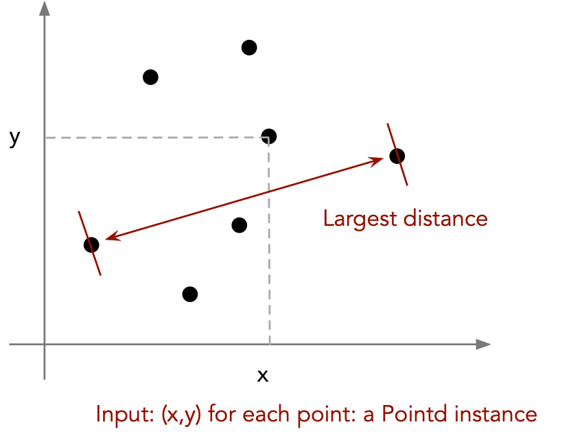
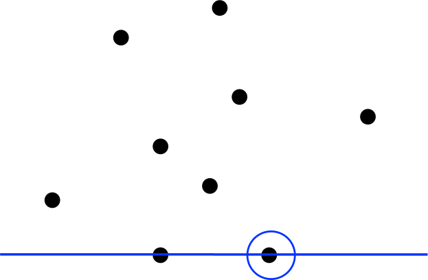
Consider the largest distance problem:

• Input: a set of points on the plane (x and y values for each point).
• Output: the distance between the two points that are furthest apart.
• Sample application: enclosure/aperture design.

In-Class Exercise 1: In this exercise you will write code to find the distance between the two furthest points among a set of points:

• Start by downloading this jar file and unpacking (use jar xvf ex1.jar at the commandline).
• Your code will go into the class MyAlgorithm
• To test, execute the LargestDistance class, specifying the number of points (to generate randomly) in the command line, as in:

  
      % java LargestDistance 50
    

• All you will need to know about the other classes is the structure of Pointd, which is simply

  
       public class Pointd {
         public double x, y;
       }
     

  to hold the x and y coordinates of a point.

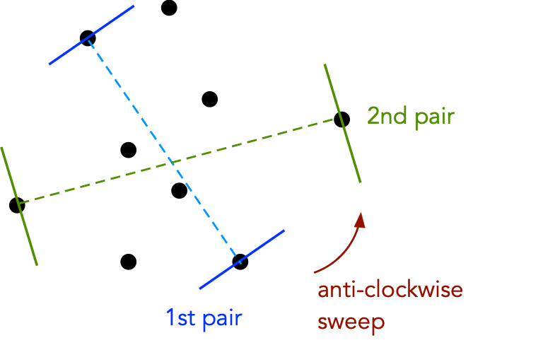
Now consider this algorithm:

• First, compute the convex hull of the set of points.
• Then, scan the hull and find antipodal pairs.
• Compute the distances between antipodal pairs.
• Report the largest such distance.

1. What is a convex hull?
   • First: a (simple) polygon is an ordered set of edges such that successive edges and only successive edges share a single endpoint.

     

   • Second: a polygon is convex if no internal angle is larger than 180 degrees.

     

   • Finally: for a set of points, the convex hull is the smallest convex polygon completely enclosing the points.

     

2. Using the Graham-Scan algorithm to compute the convex hull:
   • First find the lowest point (rightmost amongst them):

     

   • Then, compute angles to other points from the horizontal line through "lowest".

     

   • Sort points by angle.
   • Place all points temporarily in the hull.
   • Consider groups of three consecutive points, e.g.,

     

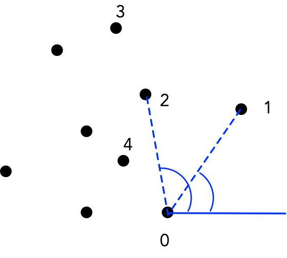
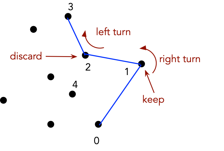
     If the center point is at a "right turn", discard that point.

   • Scan through the points once, discarding points that make a right turn.
   • Note: when discarding, you need to re-compute current group of 3 vertices (use a stack).

3. Find distances between antipodal pairs:
   • For a given vertex, its antipodals are those points that lie on parallel lines that don't cross the hull.

     

   • Key observation: the two farthest points in the set must be antipodal pairs on the hull.
   • To find these distances, compute distances from points to each hull edge:

     

   • Another key observation: antipodal pairs can be found in a single sweep
          ⇒ your clockwise neighbor's antipodal is farther along than your antipodal.

     

Now, let's take a first look at the code:

1. The AntiPodal Algorithm: (source file):

   
   public class AntiPodalAlgorithm {
   
     static double distance (Pointd p, Pointd q)
     {
       // Return the Euclidean distance between the two points. 
     }
   
     static double findMaxDistance3 (Pointd[] points, int a, int b, int c)
     {
       // Compute the distance between each of ab, ac and bc,  
       // and return the largest. 
     }
   
     boolean turnComplete = false;
   
     int nextCounterClockwise (Pointd[] points, int i)
     {
       // Find the next point in the list going counterclockwise, 
       // that is, in increasing order. Go back to zero if needed. 
       // Return the array index. 
     }
   
     int prevCounterClockwise (Pointd[] points, int i)
     {
       // Similar. 
     }
     
   
     int findAntiPodalIndex (Pointd[] hullPoints, int currentIndex, int startAntiPodalIndex)
     {
       // Given a convex polygon, an index into the vertex array (a particular vertex), 
       // find it's antipodal vertex, the one farthest away. Start the search from 
       // a specified vertex, the "startAntiPodalIndex" 
     }
   
   
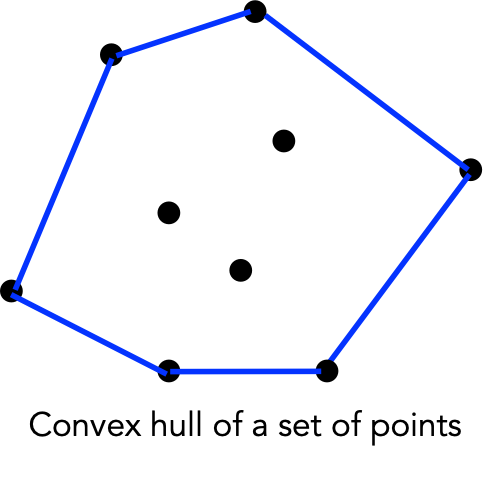
     public double findLargestDistance (Pointd[] points)
     {
       // 1. Compute the convex hull: 
       Hull hull = new Hull (points);
   
       // 2. Extract the hull points: 
       Pointd[] hullPoints = hull.getPoints();
   
       // 3. If it's exactly three points, we have a method just for that: 
       if (hullPoints.length == 3)
         return findMaxDistance3 (hullPoints, 0, 1, 2);
       
       // Otherwise, we start an antipodal scan. 
       boolean over = false;
   
       // 4. Start the scan at vertex 0, using the edge ending at 0: 
       int currentIndex = 0;
       int prevIndex = prevCounterClockwise (hullPoints, currentIndex);
   
       // 5. Find the antipodal vertex for edge (n-1,0): 
       int antiPodalIndex = findAntiPodalIndex (hullPoints, currentIndex, 1);
   
       // 6. Set the current largest distance: 
       double maxDist = findMaxDistance3 (hullPoints, currentIndex, prevIndex, antiPodalIndex);
       // We'll stop once we've gone around and come back to vertex 0. 
       double dist = 0;
       turnComplete = false;
   
       // 7. While the turn is not complete: 
       while (! over) {
   
         // 7.1 Find the next edge: 
         prevIndex = currentIndex;
         currentIndex = nextCounterClockwise (hullPoints, currentIndex);
   
         // 7.2 Get its antipodal vertex: 
         antiPodalIndex = findAntiPodalIndex (hullPoints, currentIndex, antiPodalIndex);
   
         // 7.3 Compute the distance: 
         dist = findMaxDistance3 (hullPoints, currentIndex, prevIndex, antiPodalIndex);
   
         // 7.4 Record maximum: 
         if (dist > maxDist)
           maxDist = dist;
   
         // 7.5 Check whether turn is complete: 
         if (turnComplete)
           over = true;
       } // end-while 
   
       // 8. Return largest distance found. 
       return maxDist;
   
     }
   
   
   } // End-class 
     

2. Computing the convex hull:

   
   import java.util.*;
   
   public class Hull {
   
     // Maintain hull points internally: 
     private Pointd[] hull;
   
     // The data set is given to the constructor. 
   
     public Hull (Pointd[] points)
     {
       Pointd[] vertices;
       int i, n;
   
       // Record the number of vertices: 
       n = points.length;
   
       // 1. Make a copy of the vertices because we'll need to sort: 
       vertices = new Pointd[n];
       System.arraycopy (points, 0, vertices, 0, n);
   
       // 2. Find the rightmost, lowest point (it's on the hull). 
       int low = findLowest (vertices);
   
       // 3. Put that in the first position and sort the rest by 
       //    angle made from the horizontal line through "low". 
       swap (vertices, 0, low);	
       HullSortComparator comp = new HullSortComparator (vertices[0]);
       Arrays.sort (vertices, 1, vertices.length-1, comp);
   
       // 4. Remove collinear points: 
       n = removeCollinearPoints (vertices);		
   
       // 5. Now compute the hull. 
       hull = grahamScan (vertices, n);
     }
   
     
     Pointd[] grahamScan (Pointd[] p, int numPoints)
     {
       // 1. Create a stack and initialize with first two points: 
       HullStack hstack = new HullStack (numPoints);
       hstack.push (p[0]);
       hstack.push (p[1]);
   
       // 2. Start scanning points. 
       int i = 2;
   
       // 3. While scan not complete: 
       while (i < numPoints)
       {
         // 3.1 If the current point is on the hull, push next one. 
         //     We know a point is potentially on the hull if the 
         //     the angle is convex (a left turn). 
         if ( hstack.isHull (p[i]) )
           hstack.push (p[i++]);
         //     Else remove it. 
         else
           hstack.pop ();
   
         // NOTE: the isHull() method looks for "left" and "right" turns. 
       }
   
       // 4. Return all points still on the stack. 
       return hstack.hullArray();
     }
   
     private int findLowest (Pointd[] v)
     {
       // 1. Scan through points: 
       //    1.1 If y-value is lower, the point is lower. If the y-values 
       //        are the same, check that the x value is further to the right: 
       // 2. Return lowest point found: 
     }
     
     int removeCollinearPoints (Pointd[] p)
     {
       // Not shown 
     }
     
     
     void swap (Pointd[] data, int i, int j)
     {
       // Not shown 
     }
   
   }
    

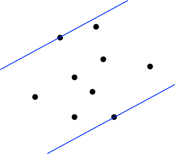
Next, consider this idea:

• Suppose experimentation reveals that the hull points are only a small subset of all the points.
  For example, we compute the number of hull points for the following data sizes (randomly generated):

  # of points	# hull points
  10	6
  100	13
  1000	18
  10000	25

• This suggests computing the hull and then doing an all-pairs distance computation: (source file):

  
  public class HullAlgorithm {
  
    static double distance (Pointd p, Pointd q)
    {
      // Return the distance between points p and q. 
    }
  
    public double findLargest (Pointd[] points)
    {
      // For each pair of points: compute the distance, recording 
      // the largest such distance: 
    }
  
    public double findLargestDistance (Pointd[] points)
    {
      // 1. Find the convex hull: 
      Hull hull = new Hull (points);
  
      // 2. Extract the points: 
      Pointd[] hullPoints = hull.getPoints();
  
      // 3. Compute an all-pairs largest-distance: 
      return findLargest (hullPoints);
    }
  
  }
    

Note:

• Fact: the AntiPodal algorithm is provably fast (fastest possible, in a worst-case sense).

• Fact: the Hull algorithm is experimentally fast, but not provably so.

• Fact: it is possible to create pathological test data that makes the Hull algorithm perform badly.

In-Class Exercise 2: What is this pathological test data? Give an example.

Summary:

• It is possible to design much faster algorithms using insight into problem structure.

• A fast algorithm may be slow for small data sets, and might require some setup overhead.

• A fast algorithm may be quite complicated, and use complex data structures.

• Some experimentation with typical data sets may reveal simpler approaches that are as effective as the provably-fast algorithms.

1.2   Improving a program's speed

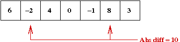
  static void algorithm1 (double[] A)
  {
    // 1. Set the initial maximum to the difference between the first two:  
    double max = Math.abs (A[0] - A[1]);

    // 2. Record the actual values: 
    double x = A[0],  y = A[1];

    // 3. Now compare each pair of numbers: 
    for (int i=0; i < A.length-1; i++){
      for (int j=i+1; j < A.length; j++) {

        // 3.1 For each such pair, see if it's difference is larger 
        //     than the current maximum. 
        double diff = Math.abs (A[i] - A[j]);

        if (diff > max) {
          // 3.1.1 If so, record the new maximum and the values 
          //       that achieved it. 
          max = diff;
          x = A[i];
          y = A[j];
        } 

      } // inner-for 
    } // outer-for 

    // 4. Output: 
    System.out.println ("Algorithm 1: the numbers: " + x + "," + y 
                        + " difference=" + max);
  }
  

    for (int i=0; i < A.length-1; i++){
      for (int j=i+1; j < A.length; j++) {
        double diff = Math.abs (A[i] - A[j]);
        if (diff > max) 
          max = diff;
      }
    }
  

    for (int i=0; i < A.length-1; i++){
      for (int j=i+1; j < A.length; j++) {
        // Instead of:
        //double diff = Math.abs (A[i] - A[j]);
        //if (diff > max) 
          //max = diff;
        // We'll represent the "work done at each step" as:
        System.out.print (" X");
      }
      System.out.println ();
    }
  

      long startTime = System.currentTimeMillis();

      // ... algorithm runs here ...
      
      double timeTaken = System.currentTimeMillis() - startTime;