In-Class Exercise 10.1:
Let's start with a little puzzle.
Examine this list of towns,
and then locate the region on Google-maps.
If you start in Springfield
(one of the towns), visit every other town exactly once, and return
to Springfield, what route (or circuit) would you chose,
assuming straight-line travel? What is the total distance traveled?
Use the Google-maps distance tool to get actual linear distances.
What are optimization problems?
- An optimization problem has "input" and a "measure"
⇒ different solutions possible, each of different value
⇒ Goal: find the "best" solution.
- The "measure" is sometimes called an objective function.
- Some problems have constraints: not all potential solutions
are "acceptable".
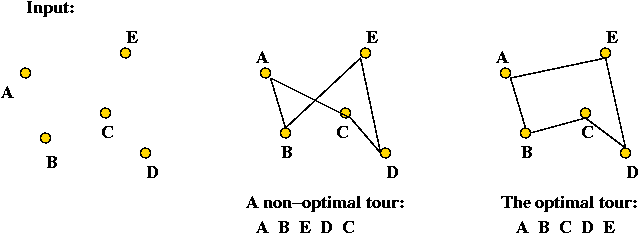
Example: the Travelling Salesperson Problem (TSP)
- Input: a collection of points (representing cities or towns).
- Goal: find a tour (circuit) of minimal length.
Length of tour = sum of inter-point distances along tour

- Details:
- Input will be a list of \(n\) points, e.g.,
\( (x_0,y_0), (x_1,y_1), \ldots, (x_{n-1},y_{n-1})\)
- Solution space: all possible tours.
- "Cost" of a tour: total length of tour.
⇒ sum of distances between points along tour
- Goal: find the tour with minimal cost (length).
- Note: strictly speaking, we have defined the Euclidean TSP.
⇒ There is also a graph version that we will not consider

- Applications:
- Logistics: trucking and delivery problems.
- Machine operation (e.g., drilling a collection of holes)
In-Class Exercise 10.2:
For an \(n\)-point problem, what is the size of the solution space
(i.e., how many possible tours are there)?
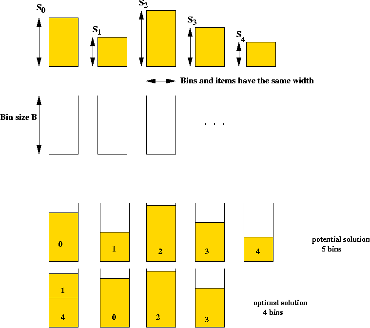
Example: the Bin Packing Problem (BPP)
- Input: a collection of items and unlimited bins.
- Items and bins have same width. Bins all have same height
(but item heights differ).
- Goal: pack the items into as few bins as possible.

- Details:
- Input is a list of \(n\) integer bin sizes
\(s_0, s_1, s_2, \ldots, s_{n-1}\)
- Solution space: all feasible packings
⇒ all assignments of items to bins such that no bin
overflows. (A constraint).
⇒ sum of sizes of items assigned to each bin is at most B.
- Goal: find the assignment that uses the fewest bins.
- Note: assume \(s_i \lt B\)
- Alternate description:
- Item sizes:
\(s_0, s_1, s_2, \ldots, s_{n-1}\)
where \(s_i \lt B\).
- Define the assignment function:
| \(d_{ij}\) |
= |
1,
0, |
if item \(i\) is placed in bin \(j\)
otherwise
|
- \(B\) = bin size.
- Goal: minimize \(k\), the number of bins
such that:
- For each \(j\),
\(s_0 d_{0j} + s_1 d_{1j} + \ldots +
s_{n-1} d_{n-1,j} \; \lt \; B\)
(all items assigned to bin \(j\) fit into the bin)
- For each \(i\),
\(\sum_{j} d_{ij} \; = \; 1\)
(each item is assigned to a bin)
In-Class Exercise 10.3:
Consider the following Bin Packing problem: there are three items with sizes
1, 2 and 3 respectively, and a bin size of 6.
Enumerate all possible assignments.
Example: Quadratic Programming Problem
- Input:
\(n\) coefficients \(a_0,a_1,\ldots,a_{n-1}\)
- Goal: minimize
\(a_0 x_0^2 + a_1 x_1^2 + a_2 x_2^2 + \ldots +
a_{n-1} x_{n-1}^2 \)
- With the constraint:
\(x_0 + x_1 + \ldots + x_{n-1} = K\)
- Here, each \(x_i\) is real-valued.
- Example:
Minimize
\(3 x_0^2 + 4x_1^2\)
Such that \(x_0 + x_1 = 10\).
In-Class Exercise 10.4:
What is the size of the set of potential solutions for
the quadratic programming problem?
Types of optimization problems:
- The Quadratic Programming problem is very different
from both TSP and BPP.
- TSP and BPP are similar is some structural respects.
- Two fundamental types of problems:
- Discrete optimization problems: finite or countable solution space.
⇒ usually finite number of potential solutions.
- Continuous optimization problems: uncountable solution space
⇒ variables are real-valued.
- Examples:
- Discrete: TSP, BPP
- Continuous: Quadratic Programming problem.
- We will focus on discrete optimization problems.
10.2
Problem Size and Execution Time
Terminology: Problem size
- Typically, the "size" of a problem is the space required to
specify the input:
- Example: TSP
⇒ For an n-point problem, space required is: O(n).
- Example: BPP
⇒ For an n-item BPP, O(n) space is required.
- Non-Euclidean TSP
- Recall: a graph is given
⇒ required to use only edges in the graph.
- A graph with n vertices can have
O(n2) edges
⇒ O(n2) space required for input.
- Consider this TSP example:
- Input: "The points are n equally spaced points on the
circumference of the unit circle".
- How much space is required for an input of 10-points? For 1000-points?
⇒ O(1) !
- The above example is not general
⇒ we need O(n) space (worst-case) to describe
any TSP problem.
Terminology: instance
- A problem instance is a particular problem (with the
data particular to that problem).
- Example: TSP on the 4 points (0, 1), (0.5, 0.6),
(2.5, 3.7) and (1, 4).
⇒ an instance of size 4.
- Another instance: TSP on the 5 points
(0, 1), (0.5, 0.6),
(2.5, 3.7), (1, 4) and (6.8, 9.1).
⇒ an instance of size 5.
Terminology: Execution time (of an algorithm)
- What we expect of an algorithm:
- An algorithm is given its input and then executed.
- The algorithm should produce a candidate solution or report
that no solutions are possible.
- Example: TSP
- An algorithm is given the set of input points.
- The algorithm should output a tour after execution.
- Example: BPP
- An algorithm is given the item sizes and bin size as input.
- The algorithm should output an assignment
(Or report that some items are too large to fit into a bin).
- Output size:
- Example: TSP
- Output is a tour
⇒ O(n) output for n points.
- Example: BPP
- Output is an assignment.
- If assignment is specified as the function
| dij |
= |
1,
0, |
if item i is placed in bin j
otherwise |
then output could be as large as O(n2).
- Execution time:
⇒ Total execution time includes processing input and writing output.
Consider these two algorithms for TSP:
- Algorithm 1:
- Initially the set P = {0, ..., n-1 } and the set
Q is empty.
- Move 0 from P to Q.
- Repeat the following until P is empty:
- Suppose k was the point most recently added to
Q.
- Find the point in P closest to k and move
that to Q.
- Output points in the order in which they were added to Q.
- Use this order as the tour.
- Algorithm 2:
- Generate a list of all possible tours and place in an array
(of tours).
- Scan array and evaluate the length of each tour.
- Output the minimum-length tour.
In-Class Exercise 10.5:
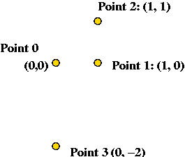
Consider the following 4 input points: (0,0), (1,0), (1,1) and
(0,-2).

- Show the steps in executing each algorithm on this input.
- What is the complexity (execution time) of Algorithm 1 on an
input of size n?
- What is the complexity of Algorithm 2 on an
input of size n?
Polynomial vs. exponential complexity:
- An algorithm has polynomial complexity or runs in
polynomial time if its execution time can be bounded by a polynomial function
of its input size.
- Example: An algorithm takes O(n3) (worst-case) on input of size
n
⇒ algorithm is a polynomial-time algorithm.
- Requirements for the polynomial:
- Highest power in the polynomial should be a constant (i.e.,
not dependent on n.
- Polynomial should be finite (not an infinite sum of terms).
- Algorithms that run slower-than-polynomial are said to have
exponential complexity:
- Typically, the (worst-case) running time is something like
O(an).
- Note: factorials have (like O(n!)) have exponential
complexity
⇒ From Stirling's formula: n! = O(sqrt(n) * (cn)n).
In-Class Exercise 10.6:
Which of these are polynomial-time algorithms?
- Algorithm 1 runs in time O( (n2 + 3)4 ).
- Algorithm 2 runs in time O(n log(n)).
- Algorithm 3 runs in time O(nn).
- Algorithm 3 runs in time O(nlog(n)).
- Algorithm 5 runs in time O( (log n)3 ).
- Algorithm 6 runs in time O( n3/n ).
Preview of things to come:
- Many important optimization problems are
discrete optimization problems.
- For these problems:
- It's easy to find simple algorithms of polynomial complexity
⇒ but that are not guaranteed to find optimal solutions.
- The only known algorithms that guarantee optimality take
exponential time.
10.3
Combinatorial Optimization Problems
A combinatorial optimization problem has three features:
- Any instance of the problem has a finite set of
states or candidate solutions S = {
s0, s1, ..., sm} .
- A cost function C defined on the states
⇒ C(s) = cost of state s.
- The problem's goal: find the state with the least cost.
Example: TSP
- Each instance of TSP is a combinatorial optimization problem.
- Example: the 4-point TSP problem with points (0,1), (1,0),
(2,3) and (3,5)
- Does this have a set of "states" or "candidate solutions"?
⇒ Yes: S = { all possible tours }
= { [0 1 2 3], [0 1 3 2], [0 2 1 3] }
- Is there a well-defined cost function on the states?
⇒ Yes: C(s) = length of tour s
e.g., C([0 1 2 3]) = dist(0,1) + dist(1,2) + dist(2,3) + dist(3,0).
- Is the goal to find the least-cost state?
⇒ Yes: find the tour with minimal length.
Example: BPP
- States: all possible assignments of items to bins.
- Cost function: C(s) = number of bins used in state s.
- Goal: find the state that uses the least bins (minimal-cost state).
In-Class Exercise 10.7:
Which of these, if any, are combinatorial optimization problems?
Identify the state space for each.
- Given a connected, weighted graph, find the minimum-spanning tree.
- Given a connected graph, discover whether it has a Hamiltonian tour.
(Recall: a Hamiltonian tour is a tour that passes through
each vertex exactly once.)
- Find the values of x1 and x2
that minimizes the function
f(x1, x2)
= x12 + x22
such that 3x1+2x2=100
- Find the values of x1 and x2
that minimizes the function
f(x1, x2)
= x12 + x22
such that 3x1+2x2≤100
and both x1 and x2 are
positive integers.
Size of a combinatorial optimization problem:
- The input is usually of size O(n) or O(n2).
- TSP: list of n points.
- BPP: n item sizes and one bin size.
- Graph-based TSP: n vertices and up to
O(n2) edges.
- MST: n vertices and up to
O(n2) edges.
- The state-space is usually exponential in size:
- TSP: all possible tours.
- BPP: all possible assignments of items to bins.
- MST: all possible spanning trees.
- The output is usually of size O(n) or
O(n2)
- TSP: a tour of size O(n)
- BPP: an assignment (matrix) of size O(n2).
- MST: an adjacency matrix of size O(n2).
10.4
Greedy Constructive Algorithms
Key ideas:
- For many combinatorial optimization problems (but not all!), it
is easy to build a candidate solution quickly.
- Use problem structure to put together a candidate solution step-by-step.
- At each step: "do the best you can with immediate information"
- Greedy constructive algorithms are usually O(n) or O(n2).
- They are constructive because they build towards
a solution in steps, starting with a small part of the problem.
Example: TSP
- Greedy Constructive Algorithm:
- Initially the set P = {0, ..., n-1 } and the set
Q is empty.
- Move 0 from P to Q.
- Repeat the following until P is empty:
- Suppose k was the point most recently added to
Q.
- Find the point in P closest to k and move
that to Q.
- Output points in the order in which they were added to Q.
- What is "greedy" about this?
- At each step, we add a new point to the existing tour.
- The new point is selected based on how close it is to
previous point.
Greedy ⇒ no backtracking.
- Execution time: O(n2) (each step requires
an O(n) selection).
- Solution quality: not guaranteed to find optimal solution.
Example: BPP
- Greedy Constructive Algorithm:
- Let A = { all items }
- Sort A in decreasing order.
- At each step until A is empty:
- Remove next item in sort-order from A.
- Find first-available existing bin to fit item.
- If no existing bin can fit the item, create a new bin and
place item in new bin.
- Running time: O(n log(n)) for sort and
O(n2) for scanning bins at each step (worst-case).
⇒ O(n2)
- Solution quality: not guaranteed to find optimal solution.
Example: MST (Minimum Spanning Tree)
- Greedy Constructive Algorithm: (Kruskal)
- Sort edges in graph in increasing order of weight.
- Process edges in sort-order:
- If adding the edge causes a cycle, discard it.
- Otherwise, add the edge to the current tree.
- Complexity: O(E log(E)) for sorting, and O(E
log(V)) for processing the edges with union-find.
⇒ O(E log(E)) overall.
- Solution quality: finds optimal solution.
About greedy constructive algorithms:
- For many problems, it's relatively easy to pose a greedy
constructive algorithm.
- For a few problems (e.g., MST), the greedy
constructive algorithm produces the
optimal solution.
- For some problems (e.g. BPP), greedy constructive algorithms produce "reasonably
good" solutions (worst-case).
- For some problems (e.g. BPP), greedy constructive algorithms produce "excellent"
solutions (in practice).
- For some problems (e.g., Hamiltonian tour), greedy constructive
algorithms are of no help at all.
10.5
Walking around the State Space
Consider the following two algorithms for TSP:
- Algorithm 1:
     // Start with input-order tour:
1.   s = initial tour 0,1,...,n-1

     // Record current best tour.
2.   min = cost(s)
3.   minTour = s

     // Repeat a large number of times:
4.   for i=1 to very-large-number
         // Create a random tour from scratch.
5.       s = generate random tour
         // See if it's better than our current best.
6.       if cost(s) < min
7.           min = cost(s)
8.           minTour = s
9.       endif
10.  endfor

     // Return best tour found.
11.  return minTour
- Algorithm 2:
     // Start with input-order tour:
1.   s = initial tour 0,1,...,n-1

     // Record current best tour.
2.   min = cost(s)
3.   minTour = s

     // Repeat a large number of times:
4.   for i=1 to very-large-number
         // Use current tour s to create next tour
5.       Pick two random points in s;
6.       s = tour you get by swapping the two selected points in s
         // See if it's better than our current best.
7.       if cost(s) < min
8.           min = cost(s)
9.           minTour = s
10.      endif
11.  endfor

     // Return best tour found.
12.  return minTour
In-Class Exercise 10.8:
Start with a 5-point TSP problem. Use some physical solution
to creating randomness (e.g, flip coins) and emulate the above two
algorithms for a few steps.
- Observe:
Each algorithm "walks around" the state space in some random fashion.
- Neighborhood:
- Define N(s) = Neighborhood(s) = { all states you can get to from
s} in any particular iteration using one of the above algorithms.
- Example: 4-point problem
- N (0123) = { all possible tours } in Algorithm 1.
- N (0123) = { 0213, 0321, 0132 } in Algorithm 2.
- A neighborhood is polynomial if the size of each
neighborhood can be bounded by a polynomial of the input size.
In-Class Exercise 10.9:
For an n-point TSP instance, what is the size of a
neighborhood in each of the above algorithms?
A different way of writing the code:
- Consider this generic "walk" in state-space:
Algorithm: stateSpaceWalk (points)
Input: n points in TSP problem
1.   s = initial tour 0,1,...,n-1
2.   min = cost(s)
3.   minTour = s
4.   for i=1 to very-large-number
         // Let method "nextState" produce the next state
5.       s = nextState(s)
6.       if cost(s) < min
7.           min = cost(s)
8.           minTour = s
9.       endif
10.  endfor
11.  return minTour
- We have seen two different nextState function's:
- Algorithm 1 above:
Algorithm: nextState (s)
Input: current state s
    // Ignore s and generate an arbitrary tour
1.  t = Generate a random tour
2.  return t
- Algorithm 2 above:
Algorithm: nextState (s)
Input: current state s
1.  t = s
2.  Pick any two random points in t
3.  Swap them.
4.  return t
Reachability:
- A "nextState" function is reachable if, from the start state,
you can eventually reach every other state by walking around long enough.
- Both "nextState" functions above are reachable.
In-Class Exercise 10.10:
Can you think of a nextState function (for TSP) that is not "reachable"?
The state-space graph:
- Consider a state s and its neighborhood of
states N(s).
- Now build a "state" graph as follows:
- The vertices of the graph are the states, like s.
- For each node s, there is a directed edge
from s to every node in N(s).
- Thus, N(s) determines the graph structure.
In-Class Exercise 10.11:
For your example in exercise 10.8, draw part of the state graph for
each of the two state-space algorithms (Algorithms 1 and 2 above),
showing the states "01234" and "10234" and their neighbors (you don't
need to draw every neighbor, just enough to show you understand
the idea).
In-Class Exercise 10.12:
Consider the Bin Packing Problem (BPP) with bins of size 5, and
the four items of sizes 1, 2, 3, 4. Start with the initial
state where each item is in a separate bin. Write pseudocode
for two potential nextState() functions for BPP,
analogous to the TSP ones above.
Then, show the neighboring states of the initial state
for the second nextState() function.
Lastly, describe a
nextState() function for BPP that's not reachable.
10.6
Greedy Local Search
Key ideas:
- A local search algorithm:
- An algorithm for a combinatorial optimization problem.
- Uses a "nextState" function to roam around the state space.
- Records the "best-solution-seen-so-far" while roaming.
- A greedy local search algorithm:
- Has little to do with "greedy constructive algorithms" described earlier.
- Uses a more intelligent "nextState" function
⇒ it examines the neighborhood, and selects the best state in
the neighborhood.
Example: greedy local search for TSP
- Idea:
- Generate a neighborhood N(s) for the current state s
- Pick the "best" (lowest-cost) state in N(s) as the
next-state.
- Repeatedly pick "best" neighbors until no neighbor is better.
- Pseudocode:
Algorithm: TSPGreedyLocalSearch (points)
Input: array of points

     // Start with any tour, e.g., in input order
1.   s = initial tour 0,1,...,n-1

     // Repeatedly find a "neighboring" tour, as long as the neighbor is better.
2.   repeat
3.       min = cost(s)
4.       minTour = s
         // Use "greedy" approach in finding a new state to walk to.
5.       s = greedyNextState(s)
6.   until cost(s) > min

     // Output best tour seen.
7.   return minTour

Output: best tour found by algorithm
Algorithm: greedyNextState (s)
Input: a tour s, an array of integers

     // Start with current tour.
1.   min = cost (s)
2.   bestNeighbor = s

     // Generate all possible neighbors by swapping two elements in s.
     // Note: go through all possible i and j systematically - O(n2) combinations
3.   for each i and j
4.       s' = swap i-th and j-th points in s
5.       if cost (s') < min
6.           min = cost (s')
7.           bestNeighbor = s'
8.       endif
9.   endfor

     // Return best one found.
10.  return bestNeighbor

Output: a tour (the best neighboring tour, using only swaps)
Greedy local search for BPP:
- Start with any assignment of items to bins.
- At each step, find the least-cost "neighboring assignment"
and make that the next assignment.
- Repeat this process until no neighbor is better.
- Computing a "neighbor":
- The current state is an assignment of items to bins.
- Try swaps between all possible pairs of bins, i and j.
- For a particular pair of bins i and j, pick an item in each
randomly and swap them.
Non-uniqueness of greedy-local-search:
- There is no "best way" to define greedy local search for a problem.
- It is possible to devise many different heuristics for
greedy local search.
- Example: alternative greedy heuristic for TSP
- Given the current tour s, consider all possible next
tours you can get by a 3-way swap.
- Example: alternative greedy heuristic for BPP
- Given current assignment, lay out items in order of
bins. Then, swap items and return to bins in first-fit order.
In-Class Exercise 10.13:
Download
TSPGreedyLocalSearchAlt.java
and
UniformRandom.java
and implement the following variation of greedy-local-search:
- Instead of trying all possible pairs (which takes
O(n2) time, we will use an O(n)-neighborhood.
-
Given the current tour, pick a random point i in the current tour.
-
Then, try all possible other points j ( j != i) to get
n-1 pairs (i,j).
- Try a swap of i and j for each of these pairs, and pick the best one.
- Return the tour resulting from the best such swap as the nextState.
10.7
Local Optima and Problem Landscape
Local optima:
- Recall: greedy-local-search generates one state (tour) after
another until no better neighbor can be found
⇒ does this mean the last one is optimal?
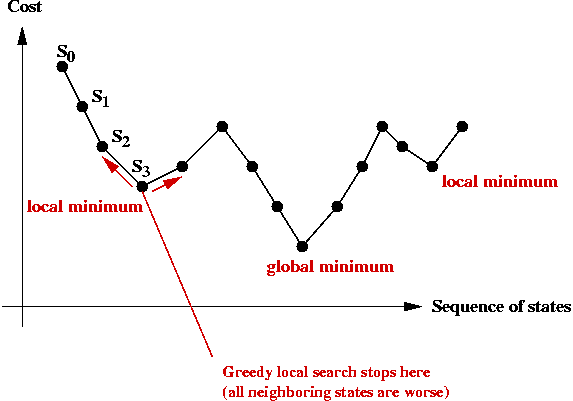
- Observe the trajectory of states:

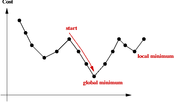
- There is no guarantee that a greedy local search can find the
(global) minimum.
- The last state found by greedy-local-search is a local minimum.
⇒ it is the "best" in its neighborhood.
- The global minimum is what we seek: the least-cost
solution overall.
- The particular local minimum found by greedy-local-search
depends on the start state:

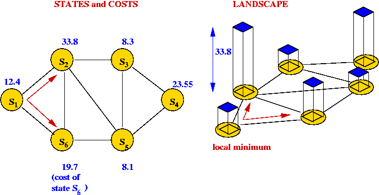
Problem landscape:
- Consider TSP using a particular local-search algorithm:
- Suppose we imagine (but not actually construct)
a graph where the vertices represent states.
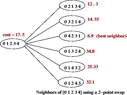
- An edge is placed between two "neighbors"
e.g., for a 5-point TSP the neighbors of [0 1 2 3 4] are:

- The cost of each tour is represented as the "weight" of each vertex.
- Thus, a local-search algorithm "wanders" around this graph.
- Picture a 3D surface representing the cost above
the graph.
⇒ this is the problem landscape for a particular problem and
local-search algorithm.

- A large part of the difficulty in solving combinatorial
optimization problems is the "weirdness" in landscapes
⇒ landscapes often have very little structure to exploit.
- Unlike continuous optimization problems, local shape in the
landscape does NOT help point towards the global minimum.
In-Class Exercise 10.14:
Consider this continuous-variable optimization
problem: minimize f(x1,x2)
= x21 + x22.
Now suppose we start with a "guess" solution
as x1=5,x2=5.
Draw a picture to show the problem landscape and where
the start solution is on the landscape.
Imagine a small neighborhood around the start solution.
What can you use to "point" towards the minimum
and start walking towards it?
Climbing out of local minima:
- A local-search algorithm gets "stuck" in a local minimum.
- One approach: re-run local-search many times with different
starting points.
- Another approach (next): help a local-search algorithm
"climb" out of local minima.
10.8*
Simulated Annealing
Background:
- What is annealing?
- Annealing is a metallurgic process for improving the
strength of metals.
- Key idea: cool metal slowly during the forging process.
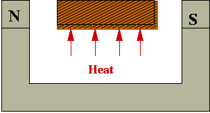
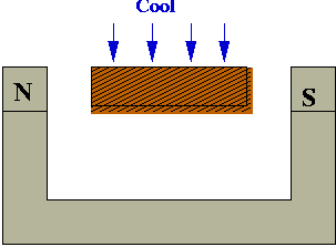
- Example: making bar magnets:
- Wrong way to make a magnet:
- Heat metal bar to high temperature in magnetic field.

- Cool rapidly (quench):

- Right way: cool slowly (anneal)
- Why slow-cooling works:
- At high heat, magnetic dipoles are agitated and move around:

- The magnetic field tries to force alignment:

- If cooled rapidly, alignments tend to be less than optimal
(local alignments):

- With slow-cooling, alignments are closer to optimal (global alignment):

- Summary: slow-cooling helps because it gives molecules more time
to "settle" into a globally optimal configuration.
- Relation between "energy" and "optimality"
- The more aligned, the lower the system "energy".
- If the dipoles are not aligned, some dipoles' fields will conflict
with others.
- If we (loosely) associate this "wasted" conflicting-fields
with energy
⇒ better alignment is equivalent to lower energy.
- Global minimum = lowest-energy state.
- The Boltzmann Distribution:
- Consider a gas-molecule system (chamber with gas molecules):

- The state of the system is the particular snapshot (positions
of molecules) at any time.
- There are high-energy states:

and low-energy states:

- Suppose the states \(s_1,s_2,\ldots\) have
energies \(E(s_1), E(s_2),\ldots\)
- A particular energy value \(E\) occurs with probability
$$\eqb{
P[E] & \eql & \mbox{Prob}[\mbox{observe energy E}] \\
& \eql & Z e^{-\frac{E}{kT}}
}$$
where \(Z\) and \(k\) are constants.
- Think of this as
$$
P[E] \;\; \propto \;\; e^{-\frac{E}{T}}
$$
- Low-energy states are more probable at low temperatures:
- Consider states \(s_1\) and \(s_2\)
with energies \(E(s_1)\) and \(E(s_2)\)
- Suppose that \(E(s_1) \lt E(s_2)\)
- The ratio of probabilities for these two states is:
$$\eqb{
r & \eql & \frac{P[E(s_2)]}{P[E(s_1)]} \\
& \eql & e^{\frac{-[E(s_2) - E(s_1)]}{kT}} \\
& \eql & \exp ({\frac{-[E(s_2) - E(s_1)]}{kT}})
}$$
In-Class Exercise 10.15:
Fill in the steps between the first and second lines above.
Then, suppose that \(E(s_1) \lt E(s_2)\) and
consider the ratio of probabilities above:
- Question: what happens to r as T increases to infinity?
- Question: what happens to r as T decreases to zero?
What are the implications?
Key ideas in simulated annealing:
- Simulated annealing = a modified local-search.
- Use it to solve a combinatorial optimization problem.
- Associate "energy" with "cost".
⇒ Goal: find lowest-energy state.
- Recall problem with local-search: gets stuck at local minimum.
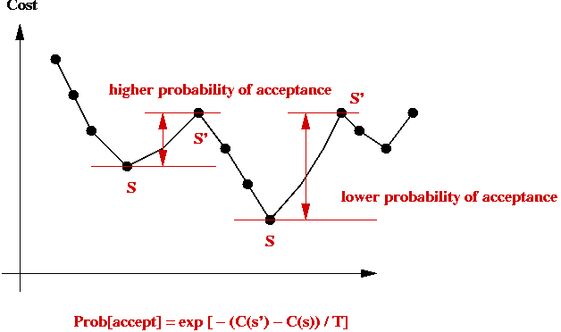
- Simulated annealing will allow jumps to higher-cost states.
- If randomly-selected neighbor has lower-cost, jump to it (like
local-search does).
- If randomly-selected neighbor is of higher-cost
⇒ flip a coin to decide whether to jump to higher-cost state
- Suppose current state is \(s\) with cost \(C(s)\).
- Suppose randomly-selected neighbor is \(s'\)
with cost \(C(s') \gt C(s)\).
- Then, jump to it with probability
$$
\exp (\frac{-[C(s') - C(s)]}{kT})
$$
- Decrease coin-flip probability as time goes on:
⇒ by decreasing temperature \(T\)
- Probability of jumping to higher-cost state depends on cost-difference:

Implementation:
- Pseudocode: (for TSP)
Algorithm: TSPSimulatedAnnealing (points)
Input: array of points

     // Start with any tour, e.g., in input order
1.   s = initial tour 0,1,...,n-1

     // Record initial tour as best so far.
2.   min = cost (s)
3.   minTour = s

     // Pick an initial temperature to allow "mobility"
4.   T = selectInitialTemperature()

     // Iterate "long enough"
5.   for i=1 to large-enough-number
           // Randomly select a neighboring state.
6.         s' = randomNextState (s)
           // If it's better, then jump to it.
7.         if cost(s') < cost(s)
8.             s = s'
               // Record best so far:
9.             if cost(s') < min
10.                min = cost(s')
11.                minTour = s'
12.            endif
13.        else if expCoinFlip (s, s')
               // Jump to s' even if it's worse.
14.            s = s'
15.        endif       // Else stay in current state.
           // Decrease temperature.
16.        T = newTemperature (T)
17.  endfor

18.  return minTour

Output: best tour found by algorithm
Algorithm: randomNextState (s)
Input: a tour s, an array of integers

    // ... Swap a random pair of points ...

Output: a tour
Algorithm: expCoinFlip (s, s')
Input: two states s and s'

1.   p = exp ( -(cost(s') - cost(s)) / T)
2.   u = uniformRandom (0, 1)
3.   if u < p
4.       return true
5.   else
6.       return false

Output: true (if coinFlip resulted in heads) or false
- Implementation for other problems, e.g., BPP
- The only thing that needs to change: define a
nextState method for each new problem.
- Also, some experimentation will be need for the temperature schedule.
Temperature issues:
- Initial temperature:
- Need to pick an initial temperature that will accept large
cost increases (initially).
- One way:
- Guess what the large cost increase might be.
- Pick initial T to make the probability 0.95 (close
to 1).
- Decreasing the temperature:
- We need a temperature schedule.
- Several standard approaches:
- Multiplicative decrease:
Use T = a * T, where a is a constant like 0.99.
⇒ Tn = an.
- Additive decrease:
Use T = T - a, where a is a constant like 0.0001.
- Inverse-log decrease:
Use T = a / log(n).
- In practice: need to experiment with different temperature
schedules for a particular problem.
Analysis:
- How long do we run simulated annealing?
- Typically, if the temperature is becomes very, very small
there's no point in further execution
⇒ because probability of escaping a local minimum is miniscule.
- Unlike previous algorithms, there is no fixed running time.
- What can we say theoretically?
- If the inverse-log schedule is used
⇒ Can prove "probabilistic convergence to global minimum"
⇒ Loosely, as the number of iterations increase, the
probability of finding the global minimum tends to 1.
In practice:
- Advantages of simulated annealing:
- Simple to implement.
- Does not need much insight into problem structure.
- Can produce reasonable solutions.
- If greedy does well, so will annealing.
- Disadvantages:
- Poor temperature schedule can prevent sufficient exploration
of state space.
- Can require some experimentation before getting it to work well.
- Precautions:
- Always re-run with several (wildly) different starting solutions.
- Always experiment with different temperature schedules.
- Always pick an initial temperature to ensure high probability
of accepting a high-cost jump.
- If possible, try different neighborhood functions.
- Warning:
- Just because it has an appealing origin, simulated annealing
is not guaranteed to work
⇒ when it works, it's because it explores more of the state
space than a greedy-local-search.
- Simply running greedy-local-search on multiple starting
points may be just as effective, and should be experimented with.
Variations:
- Use greedyNextState instead of the nextState function above.
- Advantage: guaranteed to find local minima.
- Disadvantage: may be difficult or impossible to climb out of
a particular local minimum:
- Suppose we are stuck at state s, a local minimum.
- We probabilistically jump to s', a higher-cost state.
- When in s', we will very likely jump back to
s (unless a better state lies on the "other side").
- Selecting a random next-state is more amenable to exploration.
⇒ but it may not find local minima easily.
- Hybrid nextState functions:
- Instead of considering the entire neighborhood of 2-swaps,
examine some fraction of the neighborhood.
- Switch between different neighborhood functions during iteration.
- Maintain "tabu" lists:
- To avoid jumping to states already seen before, maintain a
list of "already-visited" states and exclude these from each neighborhood.
In-Class Exercise 10.16:
Download this
template
and implement simulated annealing using the neighborhood function of
Exercise 10.13. The main-loop as well as the temperature schedule is
already in the template.
