Informal definition:
Formally:
Depicting a graph:
Graph conventions:
Definitions:
Example:
More definitions:
Known result: Euler tour exists if and only if all vertices have even degree.
Known result: testing existence of a Hamiltonian tour is (very) difficult.
Why are graphs important?
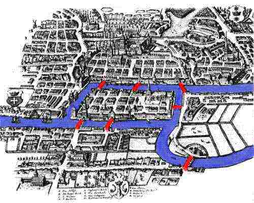
How to cross each bridge just once and return to starting point?
The field of graph theory:
In this course:
First, an idea that doesn't work:
In-Class Exercise 7.3: Draw an example graph and the corresponding pointer-based data structure. What are the pros and cons of this data structure?
The two fundamental data structures:
      0 1 1 0 0 0 0 0
      1 0 1 0 0 0 0 0
      1 1 0 1 0 1 0 0
      0 0 1 0 1 0 1 0
      0 0 0 1 0 0 1 0
      0 0 1 0 0 0 0 1
      0 0 0 1 1 0 0 0
      0 0 0 0 0 1 0 0
Note: adjMatrix[i][j] == adjMatrix[j][i] (convention for undirected graphs).
      0 1 0 0 0 0 0 0
      0 0 1 0 0 0 0 0
      1 0 0 1 0 1 0 0
      0 0 0 0 1 0 1 0
      0 0 0 0 0 0 1 0
      0 0 0 0 0 0 0 1
      0 0 0 1 0 0 0 0
      0 0 0 0 0 0 0 0
In-Class Exercise 7.4: Suppose a graph has V vertices and E edges. In order-notation (in terms of V and E), what is the size of the adjacency matrix representation? What is the size of the adjacency list representation?
In-Class Exercise 7.5: Write (parts of) a Java class to implement the adjacency list representation. Do not write all the details, but only the code for initializing the data structure. Assume the number of nodes is an integer given as parameter to the constructor.
Graph ADT:
public interface UndirectedGraphSearchAlgorithm {

  // Call this once to set up data structures.

  public void initialize (int numVertices, boolean isWeighted);


  // Call this repeatedly with each edge to be inserted:

  public void insertUndirectedEdge (int startVertex, int endVertex, double weight);


  // Return the number of connected components. If "1", then the whole
  // graph is connected.

  public int numConnectedComponents ();


  // Return the component to which each vertex belongs.

  public int[] componentLabels ();


  // Is there a cycle in the graph?

  public boolean existsCycle();

}
In-Class Exercise 7.6: How would you use this ADT to tell whether a graph is a connected tree?
Next, let's look at some sample code using the matrix representation:
public class UndirectedGraphSearch implements UndirectedGraphSearchAlgorithm {

    int numVertices;                 // Number of vertices, given as input.
    int numEdges;                    // We keep track of the number of edges.

    boolean isWeighted;              // Is this a weighted graph?

    double [][] adjMatrix;           // The matrix. Note: we use "double" to store
                                   // "double" weights, if the graph is weighted.


    public void initialize (int numVertices, boolean isWeighted)
    {
        // Store:
        this.numVertices = numVertices;
        this.isWeighted = isWeighted;

        // Create the adjacency matrix.
        adjMatrix = new double [numVertices][];
        for (int i=0; i < numVertices; i++) {
            adjMatrix[i] = new double [numVertices];
            for (int j=0; j < numVertices; j++)
                adjMatrix[i][j] = 0;
        }
        numEdges = 0;
    }


    // Insert a given input edge.

    public void insertUndirectedEdge (int startVertex, int endVertex, double weight)
    {
        // Unweighted graph: use weight 1.0.
        if (! isWeighted) {
            weight = 1.0;
        }

        // Insert in both places:
        adjMatrix[startVertex][endVertex] = weight;
        adjMatrix[endVertex][startVertex] = weight;

        numEdges ++;
    }

}
The same with an adjacency list:
public class UndirectedGraphSearch implements UndirectedGraphSearchAlgorithm {

    int numVertices;                 // Number of vertices, given as input.
    int numEdges;                    // We keep track of the number of edges.

    boolean isWeighted;              // Is this a weighted graph?

    LinkedList[] adjList;            // The list (of lists): one list for each vertex.
                                   // We are using java.util.LinkedList as our linked list.
                                   // This will store instances of GraphEdge.

    // We will test new insertions to see if they exist. Because LinkedList performs
    // ".equals()" testing for containment, we need an instance (and only one) of GraphEdge
    // for such testing.
    GraphEdge testEdge = new GraphEdge (-1, -1, 0);


    public void initialize (int numVertices, boolean isWeighted)
    {

        // Store:
        this.numVertices = numVertices;
        this.isWeighted = isWeighted;

        // Adjacency-list representation
        adjList = new LinkedList [numVertices];
        for (int i=0; i < numVertices; i++)
            adjList[i] = new LinkedList ();
            // Note: we are using java.util.LinkedList.

        numEdges = 0;

    }


    // Insert a given input edge.

    public void insertUndirectedEdge (int startVertex, int endVertex, double weight)
    {
        if (! isWeighted) {
           weight = 1.0;
        }

        // Adj-list representation: see if the edge is already there.
        testEdge.startVertex = startVertex;
        testEdge.endVertex = endVertex;

        // Exploit the methods in java.util.LinkedList.
        if (adjList[startVertex].contains (testEdge)) {
            // ... report error ...
            return;
        }

        // It's undirected, so add to both vertex lists.
        GraphEdge e = new GraphEdge (startVertex, endVertex, 1.0);
        adjList[startVertex].addLast (e);

        // We wouldn't have this for directed graphs:
        GraphEdge e2 = new GraphEdge (endVertex, startVertex, 1.0);
        adjList[endVertex].addLast (e2);

        numEdges ++;

    }

}
About graph search:
Key ideas in breadth-first search: (undirected)
Example:

In-Class Exercise 7.7:
What is the visit-order and breadth-first search tree for this graph:
Searching an unconnected graph:
The tree, and visit order:
Implementation:
Algorithm: breadthFirstMatrix (adjMatrix, n)
Input: A graph's adjacency matrix, number of vertices n.

     // Visit order will start with "0", so initialize to -1.
1.   for i=0 to n-1
2.       visitOrder[i] = -1
3.   endfor

     // A counter for the order:
4.   visitCount = -1

     // Standard queue data structure.
5.   Create queue;

     // Look for an unvisited vertex and explore its tree.
     // We need this because the graph may have multiple components.

6.   for i=0 to n-1
7.       if visitOrder[i] < 0
           // We call this "iterative" because other searches are recursive.
8.         breadthFirstMatrixIterative (i)
9.       endif
10.  endfor
Algorithm: breadthFirstMatrixIterative (u)
Input: vertex u, adjMatrix is assumed to be global.

     // Queue needs to be reset for each tree.
1.   Clear queue;

     // Place root of tree on the queue.
2.   queue.addToRear (u);

     // Continue processing vertices until no more can be added.
3.   while queue not empty

         // Remove a vertex.
4.       v = remove item at front of queue;
         // If it hasn't been visited ...
5.       if visitOrder[v] < 0
           // Visit the vertex.
6.         visitCount = visitCount + 1
7.         visitOrder[v] = visitCount
           // Look for neighbors to visit.
8.         for i=0 to n-1
9.           if adjMatrix[v][i] = 1 and i != v  // Check self-loop: i != v
                and visitOrder[i] < 0           // unvisited
10.            queue.addToRear (i)
11.          endif
12.        endfor
13.      endif

14.  endwhile
In-Class Exercise 7.8: Does the above code identify components? If so, where? If not, how can you modify the code to identify components?
A sample Java implementation: (source file)
import java.util.*;

public class UndirectedBreadthFirstMatrix {

  int numVertices;                 // Number of vertices, given as input.
  int numEdges;                    // We keep track of the number of edges.
  boolean isWeighted;              // Is this a weighted graph?
  boolean useMatrix = true;        // Adjacency-matrix or list?
  double [][] adjMatrix;           // The matrix. Note: we use "double" to store
                                   // "double" weights, if the graph is weighted.

  int[] visitOrder;                // visitOrder[i] = the i-th vertex to be visited in order.
  int visitCount;                  // We will track visits with this counter.
  LinkedList queue;                // The queue for breadth-first, a java.util.LinkedList instance.


  public void initialize (int numVertices, boolean isWeighted)
  {
    // ... We've seen this before ...
  }


  public void insertUndirectedEdge (int startVertex, int endVertex, double weight)
  {
    // ...
  }


  //-------------------------------------------------------------------------------
  // BREADTH-FIRST SEARCH


  // Initialize visit information before search.

  void initSearch ()
  {
    // IMPORTANT: all initializations will use "-1". We will test
    // equality with "-1", so it's important not to change this cavalierly.
    visitCount = -1;
    for (int i=0; i < numVertices; i++) {
      visitOrder[i] = -1;
    }
  }


  // Matrix implementation of breadth-first search.

  void breadthFirstMatrix ()
  {
    // 1. Initialize visit variables.
    initSearch ();

    // 2. Create a queue.
    queue = new LinkedList();

    // 3. Find an unvisited vertex and apply breadth-first search to it.
    //    Note: if the graph is connected, the call with i=0 will result
    //          in visiting all vertices. Nonetheless, we don't know this
    //          in advance, so we need to march through all the vertices.

    for (int i=0; i < numVertices; i++) {
      if (visitOrder[i] == -1) {
        // We call it "iterative" because depthFirst search is "recursive".
        breadthFirstMatrixIterative (i);
      }
    }

  }


  // Apply breadthfirst search to a particular vertex (root of a tree)

  void breadthFirstMatrixIterative (int u)
  {
    // 1. A fresh queue is used for a new breadth-first search.
    queue.clear();

    // 2. Start with the first vertex: add to REAR of queue using java.util.LinkedList.addLast().
    //    Because LinkedList stores objects, we "objectify" the vertex. A more efficient
    //    implementation would use a separate queue of int's.
    queue.addLast (new Integer(u));

    // 3. As long as the queue has vertices to process...
    while (! queue.isEmpty()) {

      // 3.1 Dequeue and extract vertex using java.util.LinkedList.removeFirst().
      Integer V = (Integer) queue.removeFirst();
      int v = V.intValue();

      // 3.2 If the vertex has been visited, skip.
      if (visitOrder[v] != -1)
        continue;

      // 3.3 Otherwise, set its visit order.
      visitCount++;
      visitOrder[v] = visitCount;

      // 3.4 Next, place its neighbors on the queue.
      for (int i=0; i < numVertices; i++) {
        // 3.4.1 First, check whether vertex i is a neighbor.
        if ( (adjMatrix[v][i] > 0) && (i != v) ) {

          // 3.4.1.1 If i hasn't been visited, place in queue.
          if (visitOrder[i] == -1) {
            queue.addLast (new Integer(i));
          }
        }

      } // end-for

    } // end-while

  }

} // end-class
Analysis: adjacency matrix
Analysis: adjacency list
In-Class Exercise 7.9: Why is O(V2 + E) = O(V2)? Which is better: adjacency matrix or adjacency list?
About O(V + E):
Directed graphs:
Applications:
Note: BFS works on a weighted graph by ignoring the weights and only using connectivity information (i.e., is there an edge or not?).
Key ideas:
Example:
In-Class Exercise 7.10:
What is the visit-order and depth-first search tree for this graph:
Then, apply breadth-first search, but using a stack instead of a queue.
Show the stack contents.
Implementation:
Algorithm: depthFirstMatrix (adjMatrix, n)
Input: A graph's adjacency matrix, number of vertices n.

     // Visit order will start with "0", so initialize to -1.
1.   for i=0 to n-1
2.       visitOrder[i] = -1
3.   endfor

     // A counter for the order:
4.   visitCount = -1

     // Look for an unvisited vertex and explore its tree.
     // We need this because the graph may have multiple components.
5.   for i=0 to n-1
6.       if visitOrder[i] < 0
7.         depthFirstMatrixRecursive (i)
8.       endif
9.   endfor
Algorithm: depthFirstMatrixRecursive (v)
Input: vertex v, adjMatrix is assumed to be global.

     // Mark vertex v as visited.
1.   visitCount = visitCount + 1
2.   visitOrder[v] = visitCount

     // Look for first unvisited neighbor.
3.   for i=0 to n-1
4.       if adjMatrix[v][i] > 0 and i != v
5.           if visitOrder[i] < 0
                 // If unvisited visit recursively.
6.               depthFirstMatrixRecursive (i)
7.           endif
8.       endif
9.   endfor
Algorithm: depthFirstMatrixRecursive (v)
Input: vertex v, adjMatrix is assumed to be global.

     // Mark vertex v as visited.
1.   visitCount = visitCount + 1
2.   visitOrder[v] = visitCount

     // Look for first unvisited neighbor.
3.   for i=0 to n-1
4.       if adjMatrix[v][i] > 0 and i != v  // Check self-loop.
5.           if visitOrder[i] < 0
                 // If unvisited visit recursively.
6.               depthFirstMatrixRecursive (i)
7.           endif
8.       endif
9.   endfor

     // After returning from recursion, set completion order:
10.  completionCount = completionCount + 1
11.  completionOrder[v] = completionCount
public class UndirectedDepthFirstMatrix {

  int numVertices;                 // Number of vertices, given as input.
  int numEdges;                    // We keep track of the number of edges.
  boolean isWeighted;              // Is this a weighted graph?
  boolean useMatrix = true;        // Adjacency-matrix or list?
  double [][] adjMatrix;           // The matrix. Note: we use "double" to store
                                   // "double" weights, if the graph is weighted.

  int[] visitOrder;                // visitOrder[i] = the i-th vertex to be visited in order.
  int visitCount;                  // We will track visits with this counter.
  int[] completionOrder;           // completionOrder[i] = the i-th vertex that completed.
  int completionCount;             // For tracking.


  public void initialize (int numVertices, boolean isWeighted)
  {
    // ...
  }


  public void insertUndirectedEdge (int startVertex, int endVertex, double weight)
  {
    // ...
  }


  //-------------------------------------------------------------------------------
  // DEPTH-FIRST SEARCH

  // Initialize visit information before search.

  void initSearch ()
  {
    // IMPORTANT: all initializations will use "-1". We will test
    // equality with "-1", so it's important not to change this cavalierly.
    visitCount = -1;
    completionCount = -1;
    for (int i=0; i < numVertices; i++) {
      visitOrder[i] = -1;
      completionOrder[i] = -1;
    }
  }


  // Matrix implementation of depth-first search.

  void depthFirstMatrix ()
  {
    // 1. Initialize visit variables (same initialization for breadth-first search).
    initSearch ();

    // 2. Find an unvisited vertex and apply depth-first search to it.
    //    Note: if the graph is connected, the call with i=0 will result
    //          in visiting all vertices. Nonetheless, we don't know this
    //          in advance, so we need to march through all the vertices.
    for (int i=0; i < numVertices; i++) {
      if (visitOrder[i] < 0) {
        depthFirstMatrixRecursive (i);
      }
    }
  }


  // Recursive visiting of vertices starting from a vertex.

  void depthFirstMatrixRecursive (int v)
  {
    // 1. First, visit the given vertex. Note: visitCount is a global.
    visitCount++;
    visitOrder[v] = visitCount;

    // 2. Now find unvisited children and visit them recursively.
    for (int i=0; i < numVertices; i++) {

      // 2.1  Check whether vertex i is a neighbor and avoid self-loops.
      if ( (adjMatrix[v][i] > 0) && (i != v) ) {
        if (visitOrder[i] == -1) {
          // i is an unvisited neighbor.
          depthFirstMatrixRecursive (i);
        }
      }
    }

    // 3. After returning from recursion(s), set the post-order or "completion" order number.
    completionCount++;
    completionOrder[v] = completionCount;
  }

} // end-class
"Back" and "Down" edges:
Algorithm: depthFirstMatrixRecursive (v)
Input: vertex v to be explored, adjMatrix is global.

     // Mark vertex v as visited.
1.   visitCount = visitCount + 1
2.   visitOrder[v] = visitCount

     // Look for first unvisited neighbor.
3.   for i=0 to n-1
4.       if adjMatrix[v][i] > 0 and i != v  // Check self-loop.

5.           if visitOrder[i] < 0
                 // If unvisited visit recursively.
6.               depthFirstMatrixRecursive (i)
7.           else if (i != u)  // Avoid trivial case.
8.               if visitOrder[i] < visitOrder[v]
                     // Found a back edge.
9.                   numBackEdges = numBackEdges + 1
10.              else
                     // Found a down edge.
11.                  numDownEdges = numDownEdges + 1
12.              endif
13.          endif  // visitOrder < 0

14.       endif  // adjMatrix[v][i] > 0
15.   endfor


     // After returning from recursion, set completion order:
16.  completionCount = completionCount + 1
17.  completionOrder[v] = completionCount
Identifying connected components:
Algorithm: depthFirstMatrix (adjMatrix, n)
Input: A graph's adjacency matrix, number of vertices n.

     // Visit order will start with "0", so initialize to -1.
1.   for i=0 to n-1
2.       visitOrder[i] = -1
3.   endfor

     // A counter for the order:
4.   visitCount = -1
5.   completionCount = -1
6.   currentComponentLabel = -1

     // Look for an unvisited vertex and explore its tree.
     // We need this because the graph may have multiple components.
7.   for i=0 to n-1
8.       if visitOrder[i] < 0
9.           currentComponentLabel = currentComponentLabel + 1
10.          depthFirstMatrixRecursive (i)
11.      endif
12.  endfor
Algorithm: depthFirstMatrixRecursive (v)
Input: vertex v, adjMatrix is assumed to be global.

     // Mark vertex v as visited.
1.   visitCount = visitCount + 1
2.   visitOrder[v] = visitCount

     // Mark the component label
3.   componentLabel[v] = currentComponentLabel

     // Look for first unvisited neighbor...
4.   // ... etc (same as earlier version)
In-Class Exercise 7.11:
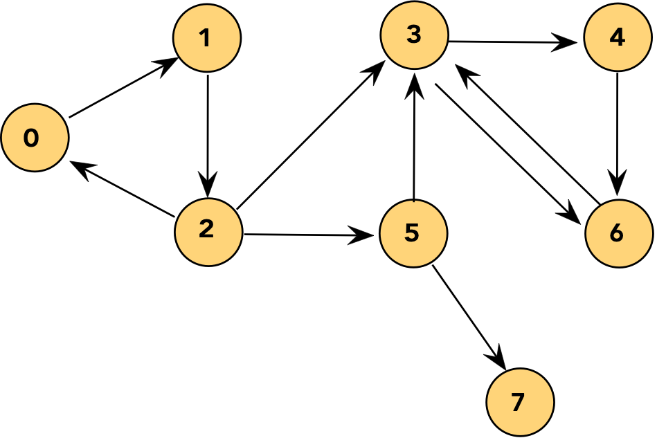
Trace the execution of DFS on the graph below to identify
exactly when the components are identified and labeled.
Analysis: adjacency matrix
Analysis: adjacency list
Applications:
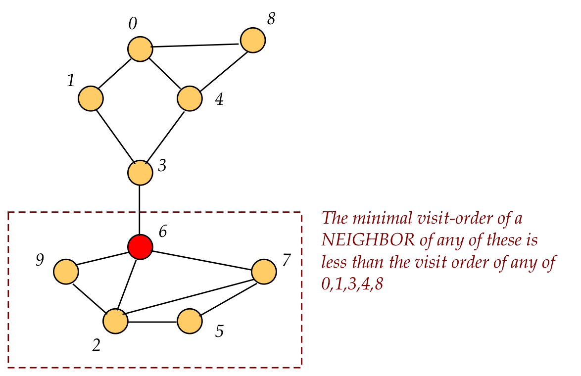
An articulation vertex is a vertex whose removal disconnects a connected graph:
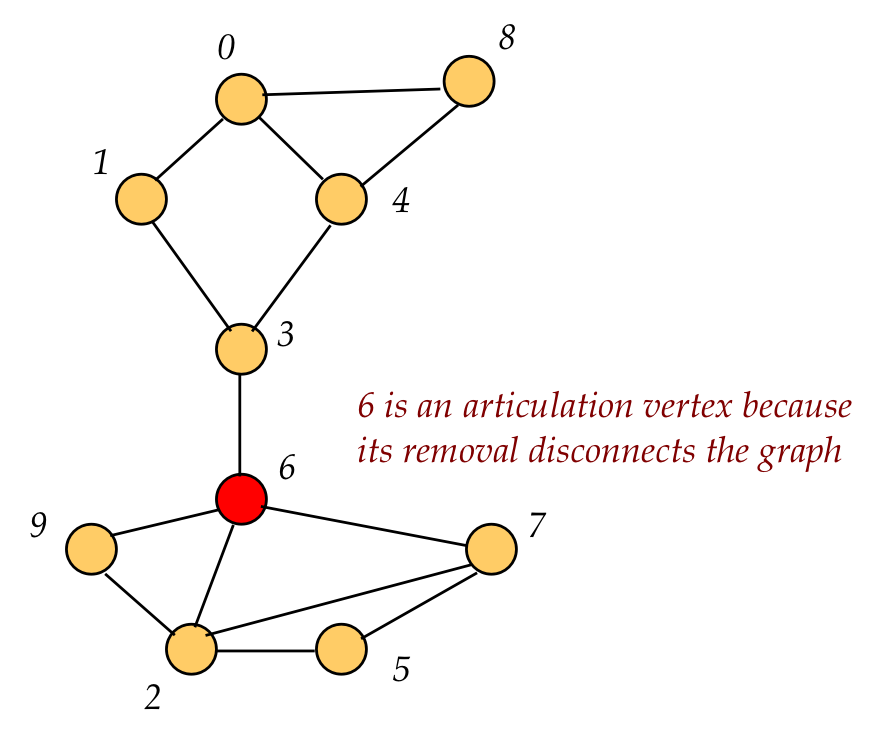
Recall visit order: the order in which DFS visits a node.
A back edge is an edge to a node that was visited earlier.
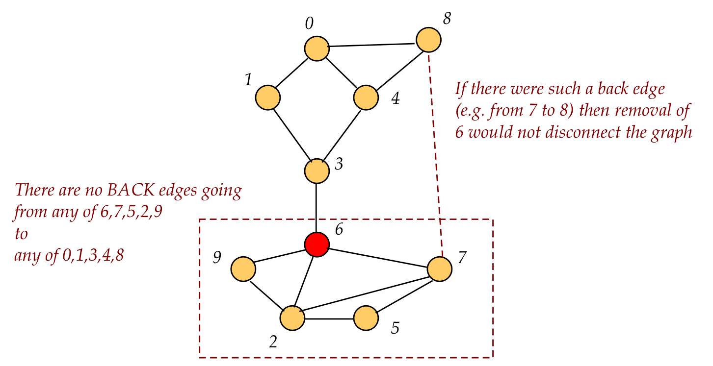
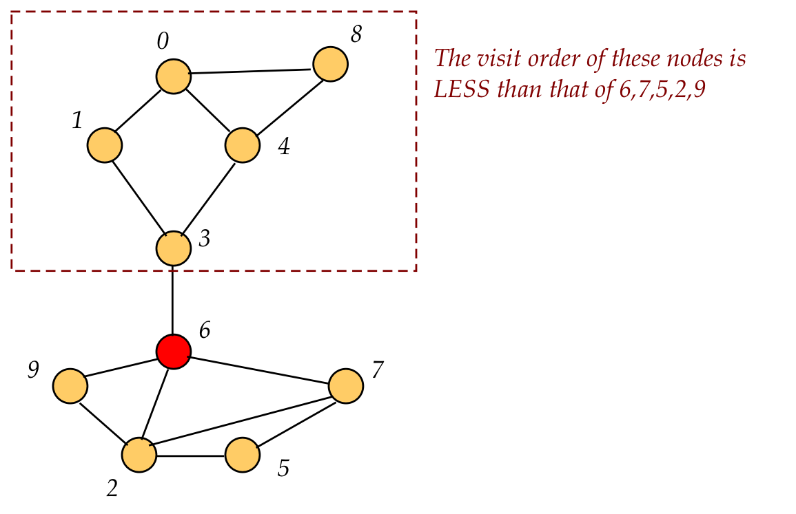
Key observation: if all nodes visited after node 6 (in this example) have no back edges to a node visited before 6, then 6 is an articulation vertex.
If, on the other hand, there were a back edge to some predecessor (in visit order) of 6, there'd be an alternative path if 6 were removed.
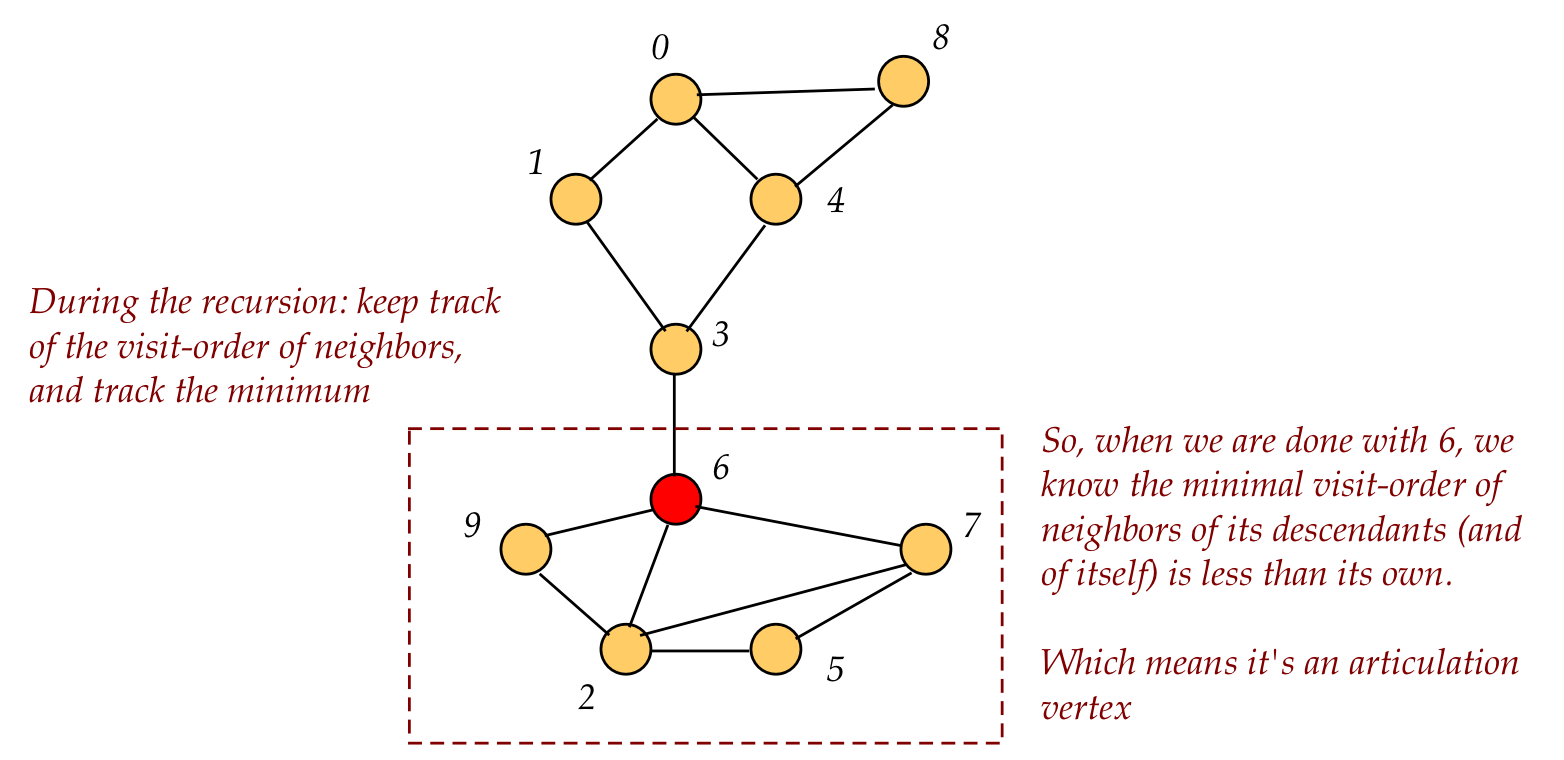
How do we track whether visit-order successors of 6 have no back edge
to its predecessors?
⇒
Track the lowest visit order amongst back edges
Thus, we'll track the minimal visit-order among back edges
we encounter as we descend in recursion and back out of recursion
⇒
Anytime the minimal is less than a node's own visit order, we've
found a back edge to a predecessor
In pseudocode:
Algorithm: depthFirstMatrixRecursive (u, v)
//Note: u is the vertex from which we reach v
1.   visitOrder[v] = ++ visitCount
2.   minBackVisitOrder = visitOrder[v]

3.   for i=0 to n-1

4.       if i is a neighbor

5.           if visitOrder[i] < 0
6.               m = depthFirstMatrixRecursive (v, i)
7.               if m ≥ visitOrder[v]
8.                   print v                       // v is an articulation vertex
9.               endif
10.              if m < minBackVisitOrder
11.                  minBackVisitOrder = m
12.              endif

13.          else if (i != u)
14.              if visitOrder[i] < visitOrder[v]  // Found a back edge.
15.                  if visitOrder[i] < minBackVisitOrder
                         minBackVisitOrder = visitOrder[i]
                     endif
16.              endif
17.          endif  // visitOrder < 0

18.       endif  // i is a neighbor

19.   endfor

20.  return minBackVisitOrder
Note:
In-Class Exercise 7.12: Trace through the algorithm above, showing the values of visitOrder[v], m and minBackVisitOrder just after line 12. What happens with vertex 0? What is a solution to the issue with vertex 0?
Key ideas:
Example:
Let's modify the pseudocode to detect cross edges as well:
Algorithm: depthFirstMatrixRecursive (u, v)
Input: the vertex u from which this is being called, vertex v
       to be explored, adjMatrix is assumed to be global.

     // Mark vertex v as visited.
1.   visitCount = visitCount + 1
2.   visitOrder[v] = visitCount

     // Look for first unvisited neighbor.
3.   for i=0 to n-1
4.       if adjMatrix[v][i] > 0 and i != v  // Check self-loop.

5.           if visitOrder[i] < 0
                 // If unvisited visit recursively.
6.               depthFirstMatrixRecursive (v, i)
7.           else if (i != u)  // Avoid trivial case.
8.               if completionOrder[i] > 0    // Finished processing i
                     // Found a cross edge.
9.                   numCrossEdges = numCrosEdges + 1
10.              else if visitOrder[i] > visitOrder[v]
                     // Found a down edge.
11.                  numDownEdges = numDownEdges + 1
12.              else
                     // Found a back edge
13.                  numBackEdges = numBackEdges + 1
14.              endif
15.          endif  // visitOrder < 0

16.       endif  // adjMatrix[v][i] > 0
17.   endfor

     // After returning from recursion, set completion order:
18.  completionCount = completionCount + 1
19.  completionOrder[v] = completionCount
Analysis: (same as undirected case)
Finding components:
In-Class Exercise 7.13: Describe in pseudocode a simple algorithm to find strongly-connected components that uses, as a part of the algorithm, the standard DFS algorithm but slightly modified for directed graphs. Hint: vertices i and j are in the same strongly-connected component if i is reachable from j and j is reachable from i. How long does your algorithm take?
We will look at two different algorithms for finding strongly-connected components:
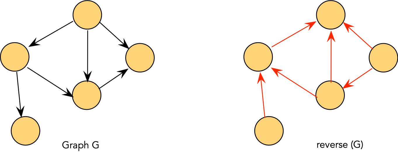
Kosaraju's algorithm:
Algorithm: stronglyConnectedComponents (adjMatrix, n)
Input: A graph's adjacency matrix, number of vertices n.
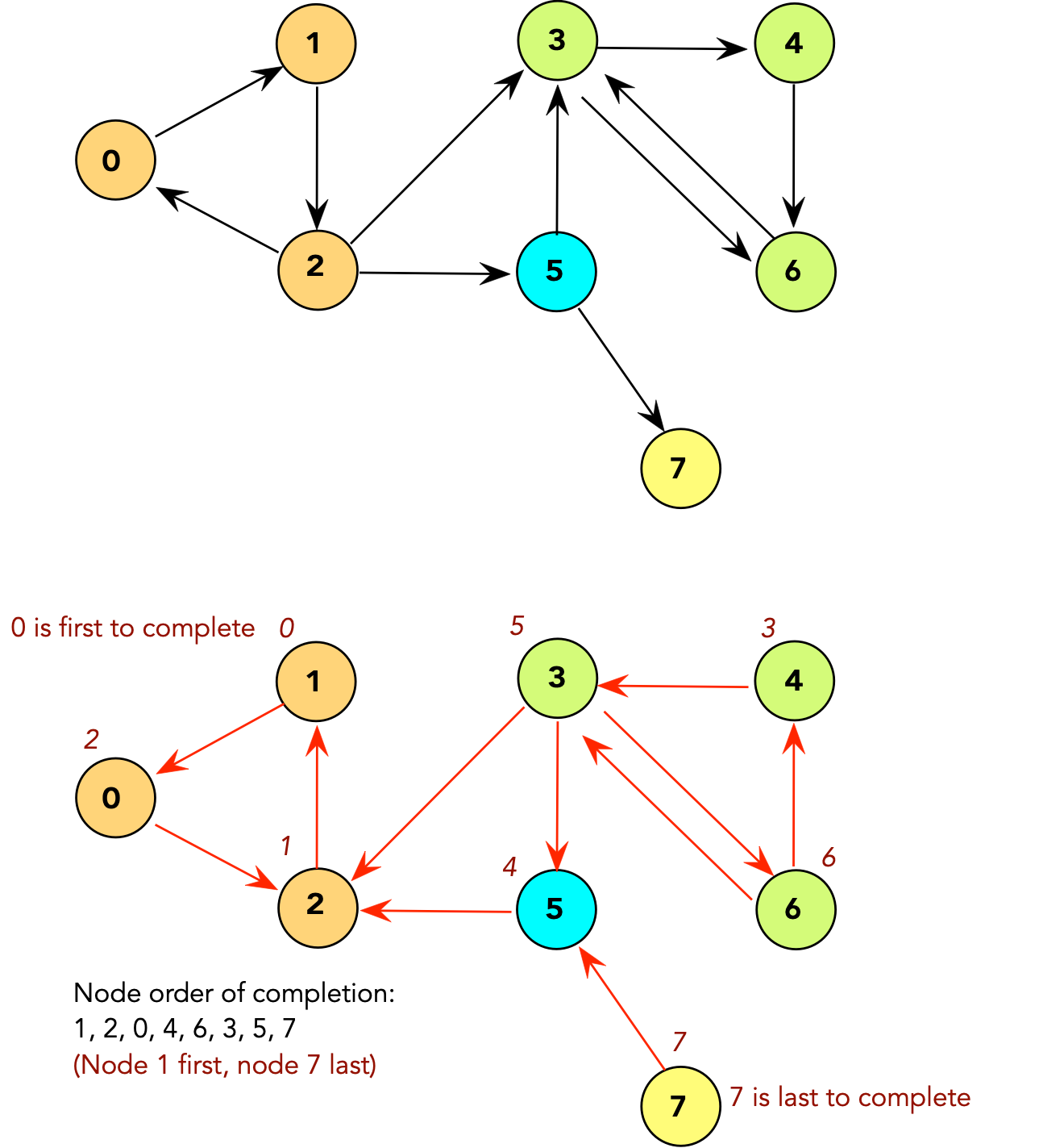
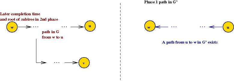
1. G' = reverse (G)
2. completionOrder = depthFirstSearch (G')
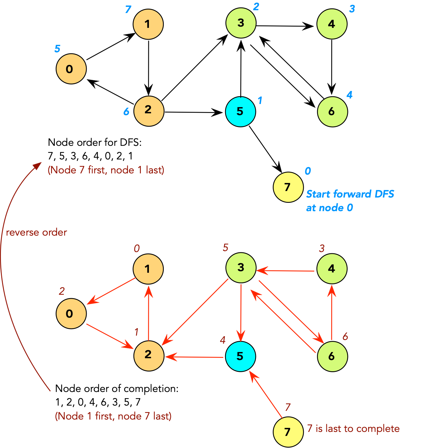
3. sortOrder = sort vertices in reverse order of completion // Last to first.
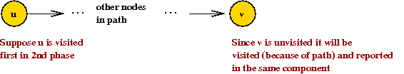
4. componentLabels = modifiedDepthFirstSearch (G, sortOrder)
5. return componentLabels
Algorithm: modifiedDepthFirstSearch (adjMatrix, sortOrder)
Input: A graph's adjacency matrix, a sort (priority) order of vertices
1. for i=0 to n-1
2. visitOrder[i] = -1
3. endfor
4. visitCount = -1
5. currentComponentLabel = -1
// Look for an unvisited vertex and explore its tree.
6. for i=0 to n-1
// Last-to-first of completion in reverse search.
7. v = sortOrder[i]
8. if visitOrder[v] < 0
9. currentComponentLabel = currentComponentLabel + 1
10. modifiedDepthFirstMatrixRecursive (v)
11. endif
12. endfor
13. return componentLabels
Algorithm: modifiedDepthFirstMatrixRecursive (v)
// Mark vertex v as visited and record component label.
1. visitCount = visitCount + 1
2. visitOrder[v] = visitCount
3. componentLabel[v] = currentComponentLabel
// Look for first unvisited neighbor.
4. for i=0 to n-1
u = sortOrder[i] // Prioritize in sort-order
5. if adjMatrix[v][u] > 0 and u != v
6. if visitOrder[u] < 0
7. depthFirstMatrixRecursive (u)
8. endif
9. endif
10. endfor
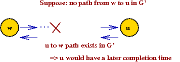
⇒ Then, the path from u to w in G' would
result in u having a later completion time
⇒ Contradiction.
Let's look at the second (harder to understand) algorithm that finds strongly connected components.
Algorithm: depthFirstMatrixRecursive (u, v)
Input: the vertex u from which this is being called, vertex v
       to be explored, adjMatrix is assumed to be global.

     // Mark vertex v as visited.
1.   visitCount = visitCount + 1
2.   visitOrder[v] = visitCount

     // Current lowest reachable:
3.   lowestReachable[v] = visitOrder[v];

     // Important: minLowestReachable is a local variable so that a
     // fresh version is used in each recursive call.
4.   minLowestReachable = lowestReachable[v];

     // Initialize stackTop to 0 outside. stackTop points to next available.
5.   stack[stackTop] = v;
6.   stackTop ++;

     // Look for first unvisited neighbor.
7.   for i=0 to n-1
8.       if adjMatrix[v][i] > 0 and i != v  // Check self-loop.

9.           if visitOrder[i] < 0
                 // If unvisited visit recursively.
10.              depthFirstMatrixRecursive (v, i)
11.          else if (i != u)  // Avoid trivial case.
                 // Identify back, down and cross edges ... (not shown)
12.          endif  // visitOrder < 0

13.          if lowestReachable[i] < minLowestReachable
14.              minLowestReachable = lowestReachable[i]
15.          endif

16.      endif  // adjMatrix[v][i] > 0
17.   endfor

     // We reach here after all neighbors have been explored.
     // Check whether a strong component has been found.
18.  if minLowestReachable < lowestReachable[v]
         // This is not a component, but we need to update the
         // lowestReachable for this vertex since its ancestors will
         // use this value upon returning.
19.      lowestReachable[v] = minLowestReachable
20.      return
21.  endif

     // We've found a component.
22.  do
         // Get the stack top.
23.      stackTop = stackTop - 1
24.      u = stack[stackTop];
         // We start currentStrongComponentLabel from "0".
25.      strongComponentLabels[u] = currentStrongComponentLabel;
         // Set this to a high value so that it does not affect
         // further comparisons up the DFS tree.
26.      lowestReachable[u] = numVertices;
27.  while stack[stackTop] != v

28.  currentStrongComponentLabel = currentStrongComponentLabel + 1
     // After returning from recursion, set completion order... (not shown)
What are they?

Sequential scheduling:
Topological sort:
In-Class Exercise 7.14: Apply the classic algorithm to the above example.
Using depth-first search:

Pseudocode:
Algorithm: depthFirstMatrixRecursive (u, v)
Input: the vertex u from which this is being called, vertex v
       to be explored, adjMatrix is assumed to be global.

     // Mark vertex v as visited.
1.   visitCount = visitCount + 1
2.   visitOrder[v] = visitCount

     // Look for first unvisited neighbor and recurse
3.   for i=0 to n-1
          // ... (same as before, not shown) ...
4.   endfor

     // After returning from recursion, set completion order:
5 .  completionCount = completionCount + 1
6.   completionOrder[v] = completionCount

     // Set topological sort order.
     // Initialize topSortCount to -1 outside this method
7.   topSortCount = topSortCount + 1
8.   topSortOrder[topSortCount] = v