By the end of this module, you will be able to:
- Explain the difference between online and offline algorithms.
- Demonstrate how union-find works, with an example.
- Analyze the time-complexity of the union-find algorithms described in the module.
- Apply union-find to the problem of finding components in a graph.
- Explain the shortest-path and minimum-spanning tree problems for weighted graphs.
- Demonstrate via an example how Kruskal's and Prim's algorithms compute the MST.
- Explain how a priority queue is used in Prim's algorithm, and why it's used.
- Explain how Dijkstra's algorithm works, via an example.
- Analyze the running time of Kruskal's, Prim's and Dijkstra's algorithms.
8.1 On-line versus Off-line Problems
Consider the Graph-Component problem we've looked at before:
- Input: "relationship pairs", e.g.
(A, B) (D, E) (B, A) (E, D) (A, C) - Desired output: identify the connected components
- Sometimes, these are also called equivalence classes
(the language used in the earlier discrete-math course)
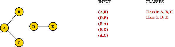
- Thus, output for this example:
    class 0: A, B, C
    class 1: D, E
Off-line version:
- Entire input is given at once.
- Solution:
- Scan input and place edges in undirected graph.
- Run depth-first search to identify components and label each vertex.
- Scan labels and print out classes (components).
- Analysis: O(V + E).
(Here, E = number of input pairs.)
On-line version of problem:
- Note: The meaning of online here has nothing to do with being "online."
- First, number of elements (vertices) is given to the algorithm.
- Then, the algorithm receives one pair (edge) at a time.
- The algorithm must output currently known components (equivalence classes) at each step.
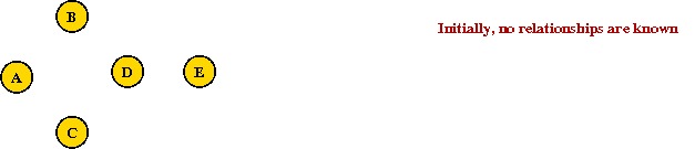
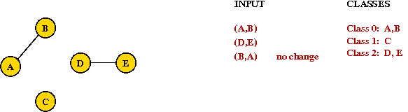
- Consider this example with 5 nodes
- Initially, each node is in its own "class" or "group":
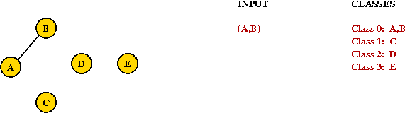
- With input (A,B):
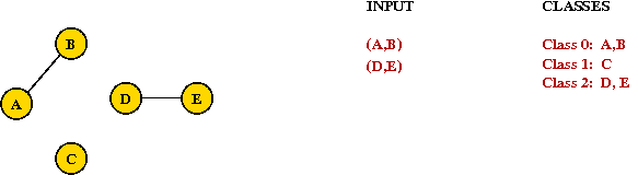
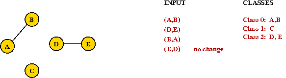
- Next input: (D,E):
- Next input: (B,A):
- Next input: (E,D):
- Next input: (A,C):
- Initially, each node is in its own "class" or "group":
About on-line problems:
- Input is usually a "sequence of data values".
(Called request sequence). - Input is revealed one piece at a time.
- Algorithm must output current (partial) solution after each input.
- Algorithm cannot know future input in the sequence.
- Algorithm is allowed to use past input.
- Data is allowed to repeat, e.g., "vertices" and "edges" repeat in edge sequence.
- Typical analysis:
- Given an input sequence of size m about n items, what is the time taken in terms of m and n?
- The term on-line has nothing to do with the usual meaning of "on-line".
Using depth-first search for the on-line graph-component problem:
- After reading each "edge", run depth-first search to identify components.
In-Class Exercise 8.1: For n vertices and a sequence of m edges, how long does the above algorithm take to process the whole sequence?
8.2 Union-Find Algorithms: Solving the On-line Graph-Component Problem
Key ideas:
- The graph-component problem can expressed a little
differently
⇒ the Union-Find Problem. - Union-Find:
- Given: initial collection of "singleton" sets, e.g.
A, B, C, D, E - Input: sequence of (possibly interspersed) "union" or "find" operations, e.g.,
union (A, B) find (A) find (C) union (D, E) union (B, A) find (D) find (E) union (E, D) union (A, C) find (C) find (A) - Here
union(A,B) means: join the communities of A and B into one
find(A) means: output A's community (as much as known thus far) - Output: return the current set identifier (which component)
after each "find" operation, e.g.,
    union (A, B)
    find (A)
    Output: set 0

    find (C)
    Output: set 1

    union (D, E)
    union (B, A)
    find (D)
    Output: set 2

    find (E)
    Output: set 2

    union (E, D)
    union (A, C)
    find (C)
    Output: set 0

    find (A)
    Output: set 0
- Given: initial collection of "singleton" sets, e.g.
In-Class Exercise 8.2:
What is the output after each find operation in
the following sequence on nodes A through H, assuming
no knowledge of any edges at the start?
  union (A, B)
  union (A, C)
  find (C)
  find (D)
  union (G, H)
  union (F, G)
  find (H)
  union (C, F)
  find (H)
ADT (Abstract Data Type) for a union-find algorithm:
- With the communities problem, think of the nodes of the graph
as people, in which case the ADT would look like:
public interface UnionFindAlgorithm { // Initialize with number of people (e.g., number of vertices) public void initialize (int maxPersons); // Call this repeatedly to initialize each person as its own set (group). public void makeSingleElementSet (int person); // Union operation. public void union (int person1, int person2); // Find operation: returns the ID of the set (group) that currently contains the given person. public int find (int person); } - For other problems that feature integer-items: we would use
public interface UnionFindAlgorithm {

  // Initialize with number of items (e.g., number of vertices)
  public void initialize (int maxItems);

  // Call this repeatedly to instantiate initial sets.
  public void makeSingleElementSet (int item);

  // Union operation.
  public void union (int item1, int item2);

  // Find operation: returns the ID of the set that currently contains "item".
  public int find (int item);

}
The Quick-Find Algorithm:
- Assume: data consists of integers (0, 1, 2, ...)
(Node labels or person IDs) - Key ideas:
- Maintain set ID's in an array:
- Every union operation merges two sets (groups)
⇒ they need to have the same set ID (community ID)
⇒ write first set ID over the set ID's of second set members:
- Find operation: simply return set ID.
- Maintain set ID's in an array:
- Analysis:
- Find operation: O(1)
- Union operation: O(n) (worst-case)
- For m operations on n items: O(mn) worst-case.
- Pseudocode:
Algorithm: union (item1, item2) Input: two items, whose sets are to be combined. // Important: Assume initialization is complete, and ID[i] = i initially. // If they are in the same set, nothing to be done. 1. if ID[item1] = ID[item2] 2. return 3. endif // Otherwise, change the ID of every member in the second set to ID[item1] 4. id2 = ID[item2] 5. for i=0 to numItems-1 6. if ID[i]=id2 7. ID[i] = ID[item1] 8. endif 9. endforAlgorithm: find (item) Input: an item whose set ID needs to be returned // ID's are always up-to-date, so return the current set ID. 1. return ID[item] Output: ID of current set that "item" belongs to.
In-Class Exercise 8.3:
Look closely at the pseudocode in union above. Why doesn't
the following work?
     // Otherwise, change the ID of every member in the second set to ID[item1]
5.   for i=0 to numItems-1
6.       if ID[i]=ID[item2]
7.           ID[i] = ID[item1]
8.       endif
9.   endfor
The Leader metaphor:
- Suppose each set ID represents a "set leader".
- Leaders can be represented using the items themselves.
- "Find" operation: return leader's name (ID).
- "Union" operation: make two sets have the same leader (same ID).
e.g., merge {0, 1} and {2, 4}.
⇒ hierarchy: leaders have leaders - Maximum leader: an item who has no leader (points to itself).
- Hierarchical view:
The Quick-Union Algorithm:
- Idea: try to make "union" faster at the expense of a longer "find".
- Union:
- Find the maximum leader of each set.
- Make one leader subservient (point to) to the other.
- Find:
- Find the maximum leader, and return ID.
- Pseudocode:
Algorithm: union (item1, item2) Input: two items, whose sets are to be combined. // Important: Assume initialization is complete, and ID[i] = i initially. // If they are in the same set, nothing to be done. 1. if ID[item1] = ID[item2] 2. return 3. endif // Identify the two maximum leaders of the sets (which could be the same) 4. leader1 = find (item1) 5. leader2 = find (item2) // Either one of the assignments below will do. However, we can // generate as low a set-numbering as possible with this extra // O(1) computation. 6. if leader1 < leader2 7. ID[leader2] = ID[leader1] 8. else 9. ID[leader1] = ID[leader2] 10. endifAlgorithm: find (item) Input: an item whose set ID needs to be returned // Start with the leader of the value (which may point to itself). 1. nextLeader = ID[item] // Go up the hierarchy to the (unique) maximum leader of this set. // The maximum leader will point to itself. 2. while ID[nextLeader] != nextLeader 3. nextLeader = ID[nextLeader] 4. endwhile // Return the leader itself. 5. return nextLeader Output: ID of current set that "item" belongs to. - A potential problem with Quick-Union:
- Consider the set {0, 1, 2, 3, 4, 5, 6, 7}.
- And these operations:
union (7, 6) union (6, 5) union (5, 4) union (4, 3) union (2, 1) union (1, 0) union (3, 2) - Resulting hierarchy:
- Analysis:
- Worst-case: long tree (O(n) depth).
- Repeat "bad union" operations:
⇒ O(n2)
Weighted-Union:
- Key idea: keep the trees balanced!
- Two approaches:
- Randomize choice of leader.
- Make leader of smaller tree point to leader of larger tree.
⇒ requires "size" storage.
- Weighted-Union pseudocode:
Algorithm: union (item1, item2) Input: two values, whose sets are to be combined. // Important: Assume initialization is complete, and ID[i] = i // and groupSize[i] = 1 initially. // If they are in the same set, nothing to be done. 1. if ID[item1] = ID[item2] 2. return 3. endif // Identify the two maximum leaders of the sets (which could be the same) 4. leader1 = find (item1) 5. leader2 = find (item2) // Make the smaller group point to the larger and update the // group size of the larger group. 6. if groupSize[leader1] < groupSize[leader2] 7. ID[leader1] = ID[leader2] 8. groupSize[leader2] = groupSize[leader2] + groupSize[leader1] 9. else 10. ID[leader2] = ID[leader1] 11. groupSize[leader1] = groupSize[leader1] + groupSize[leader2] 12. endifAlgorithm: find (item) Input: an item whose set ID needs to be returned // ... same as in Quick-Union algorithm ... (not shown here) Output: ID of current set that "value" belongs to. - Example:
- Same sequence as before.
- Same sequence as before.
- Analysis:
- Worst-case depth of tree: O(log(n)) (tree is
approximately balanced).
(To see why, follow pointers down to smaller sets - reduces size by at least half each time). - Since the worst-case for an operation (find) is O(log(n)), a sequence of k operations takes at most O(k log(n)).
- Worst-case depth of tree: O(log(n)) (tree is
approximately balanced).
A small improvement to "find": (path compression)
- Each time "find" is invoked on a value, adjust its leader to
point to "leader's leader".
⇒ halve the path to root with each find operation
⇒ cuts down depth by half. - Each "halving" action costs O(1).
⇒ over time, it reduces depth. - Complicated analysis shows: O(m A(m,n)) time
where A(m,n) is inverse-Ackerman's function
⇒ a really slow-growing function.
In-Class Exercise 8.4:
Solve the Communities
Problem using union-find as operations. For your actual code,
use any union-find approach above, but for reasoning, we'll focus
on the weighted-union approach.
8.3 Weighted Graphs
Weighted graphs:
- Thus far, we have only considered un-weighted graphs, e.g.,
- In a weighted graph, (usually) the edges have weights:
- In applications, edge weights usually reflect something like:
- The actual distance (geometric).
- The cost (installation or rental cost).
- Reliability, transmission speed, etc.
- Directed graphs:
- Each edge has direction.
- Even if two vertices have two opposing edges, edge weights can differ (depending on application).
- Generally, the algorithms for undirected (weighted) graphs that we will encounter will port over (with minor changes) to directed graphs.
- Where are weights stored?
- In adjacency-matrix representation, adjMatrix[i][j] = weight of edge (i,j)
- In adjacency-list representation, store weight in linked list nodes.
Two important problems with weighted graphs:
- The Minimum Spanning Tree (MST) Problem:
- Input: a weighted, connected graph.
- Objective: find a sub-graph such that:
- The sub-graph is a connected tree.
- The tree contains all graph vertices.
⇒ it's a spanning tree. - The tree weight is defined as the sum of edge-weights in the tree.
- The tree weight is the least among such spanning trees.
- The Shortest Path Problem:
- Input: a weighted, connected graph.
- Objective: find a path between every pair of vertices such
that:
- The path-weight is defined as the weight of edges in the path.
- The path-weight for a particular pair is the least among all such paths (for the pair).
In-Class Exercise 8.5:
"Eyeball" the weighted graph below
and find the minimum spanning tree, and the shortest path from vertex 0
to vertex 6. Can you find another spanning tree that's not minimal,
and an alternate non-optimal path from 0 to 6?
Write down or draw the adjacency matrix and adjacency list for the
above graph. Next, a drawing exercise in preparation for the next section:
draw a dashed line and then, redraw the above graph so that
the even-numbered vertices are drawn on the left side of the
dashed line, and the other vertices are on the right side.
8.4 Minimum Spanning Trees: Two Key Observations
The Cut-Edge Observation:
- Consider a partition of the vertices into two sets.
- Suppose we re-draw the graph to highlight edges going from
one set to the other: (without changing the graph itself)
- Cut-edge: an edge between the two sets.
- Consider the minimum-weight edge between the sets.
(Assume the edge is unique, for now). - The minimum-weight edge must be in the minimum spanning tree.
In-Class Exercise 8.6: Why?
Prim's algorithm (a preview):
- Start with Set1 = {vertex 0}, Set2 = {all others}.
- At each step, find an edge (cut-edge) of minimum-weight between the two sets.
- Add this edge to MST and move endpoint from Set2 into Set1.
- Repeat until Set1 = {all vertices}.
The Cycle Property:
- First, note: adding an edge whose end-points are in the MST will always cause a cycle.
- Consider adding an edge that causes a cycle in current MST.
- Suppose the edge has weight larger than all edges in cycle
⇒ no need to consider adding edge to MST.
- Therefore, if edges are added in order of (increasing)
weight
⇒ no need to consider edges that cause a cycle.
Kruskal's algorithm (a preview):
- Sort edges in order of increasing weight.
- Process edges in sort-order.
- For each edge, add it to the MST if it does not cause a cycle.
8.5 Kruskal's Algorithm
Key ideas:
- Sort edges by (increasing) weight.
- Initially, each vertex is a solitary sub-graph (MST-component).
- Start with small MST-component's and grow them into one large MST.
- Need to track: which vertex is in which component (i.e., set).
Example:
- Initially:
- Sort order of edges:
(2, 3), (0, 1), (3, 4), (1, 3), (4, 6), (3, 6), (1, 2), (0, 2), (2, 5), (5, 7) - First edge to add joins "2" and "3" (no cycle):
- Next edge in sort order: (0, 1):
- Next edge in sort order: (3, 4):
- Next edge in sort order: (1, 3): merges two sets (union)
- Next edge in sort order: (4, 6):

- Next edge in sort order: (3, 6): cannot be added
- Next two edges also cannot be added: (0, 2) and (1, 2).
- Finally, add (2, 5) and (5, 7):
In-Class Exercise 8.7:
Use Kruskal's algorithm, showing all the steps (with drawings of
both the graph and the node-sets)
to find the MST of this graph:
Implementation:
- High-level pseudocode:
Algorithm: Kruskal-MST (G)
Input: Graph G=(V,E) with edge-weights.

1.   Initialize MST to be empty;
2.   Place each vertex in its own set;
3.   Sort edges of G in increasing-order;
4.   for each edge e = (u,v) in order
5.       if u and v are not in the same set
6.           Add e to MST;
7.           Compute the union of the two sets;
8.       endif
9.   endfor
10.  return MST

Output: A minimum spanning tree for the graph G.
- Now, let's use a union-find algorithm and explain in more
detail:
Algorithm: Kruskal-MST (adjMatrix)
Input: Adjacency matrix: adjMatrix[i][j] = weight of edge (i,j) (if nonzero)

1.   Initialize MST to be empty;

     // Initialize union-find algorithm and
     // place each vertex in its own set.
2.   for i=0 to numVertices-1
3.       makeSingleElementSet (i)
4.   endfor

5.   sortedEdgeList = sort edges in increasing-order;

6.   Initialize treeMatrix to store MST;

     // Process edges in order.
7.   while sortedEdgeList.notEmpty()
8.       edge (i,j) = extract edge from sortedEdgeList.
         // If edge does not cause a cycle, add it.
9.       if find(i) != find(j)
10.          union (i, j)
11.          treeMatrix[i][j] = treeMatrix[j][i] = adjMatrix[i][j]
12.      endif
13.  endwhile

14.  return treeMatrix

Output: adjacency matrix represention of tree.
Analysis: (adjacency matrix)
- Placing edges in list: requires scan of adjacency matrix
⇒ O(V2). - Sorting edges: O(E log(E)).
- One union-find operation for each edge: O(E log(V)).
- Total: O(V2) + O(E log(E)) + O(E log(V))
⇒ O(V2), for sparse graphs
⇒ O(V2)log V, for dense graphs
Analysis: (adjacency list)
- To place edges in list: simply scan each vertex list once.
⇒ O(E) time. - Total: O(E)+ O(E log(E)) + O(E log(V))
⇒ O(E log(E))
⇒ O(E log(V)) (same for sparse or dense)
In-Class Exercise 8.8: Explain the statements for the adjacency list above (the time taken for sparse and dense graphs). Why is O(E log(E)) = O(E log(V))? Is the adjacency list always better than an adjacency matrix for this problem?
8.6 Prim's Algorithm
Key ideas:
- Start with vertex 0 and set current MST to vertex 0.
- At each step, find lowest-weight edge from an MST vertex to a non-MST vertex and add it to MST.
- To record the weight of each edge, we will associate edge weight with the vertex that's outside the MST.
- We will associate a priority with each vertex:
⇒ intuitively, priority of vertex v = "currently known cost of adding v to MST" - Example:
- A partially built tree:
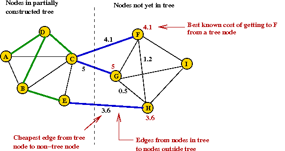
- Priorities change after H is added to tree:
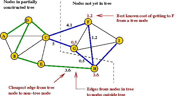
- A partially built tree:
Example:
- Initially, place vertex 0 in the MST and set the "priority" of
each vertex to infinity.
- Explore edges from current MST: (0, 1) and (0, 2).
- Pick lowest-weight edge (0, 1) to add
⇒ same as selecting lowest-priority vertex (vertex 1)
- Explore edges from newly-added vertex: (1,3), (1,2)
That's why we associate edge-weights with vertices
⇒ only the edges from the new vertex add new information at each step. - Pick vertex with lowest priority (vertex 3) and explore its edges:
- Continuing, we add vertices 2, 4, 6, 5 and 7:
In-Class Exercise 8.9:
Use Prim's algorithm, showing all the steps
(especially node labels) to find the MST of this graph:
Record all those instances where the priority decreased from
a non-infinite value to something lower.
Implementation:
- High-level pseudocode:
Algorithm: Prim-MST (G) Input: Graph G=(V,E) with edge-weights. 1. Initialize MST to vertex 0. 2. priority[0] = 0 3. For all other vertices, set priority[i] = infinity 4. Initialize prioritySet to all vertices; 5. while prioritySet.notEmpty() 6. v = remove minimal-priority vertex from prioritySet; 7. for each neighbor u of v // See if the priority of u changes because of v. 9. w = weight of edge (v, u) 8. if w < priority[u] 9. priority[u] = w 10. endif 11. endfor 12. endwhile Output: A minimum spanning tree of the graph G. - More detailed pseudocode: (adjacency matrix)
Algorithm: Prim-MST (adjMatrix)
Input: Adjacency matrix: adjMatrix[i][j] = weight of edge (i,j) (if nonzero)

     // inMST[i] = true once vertex i is in the MST.
1.   Initialize inMST[i] = false for all i;
2.   Initialize priority[i] = infinity for all i;
3.   priority[0] = 0
4.   numVerticesAdded = 0

     // Process vertices one by one. Note: priorities change as we proceed.
5.   while numVerticesAdded < numVertices
       // Extract best vertex.
6.       v = vertex with lowest priority that is not in MST;
         // Place in MST.
7.       inMST[v] = true
8.       numVerticesAdded = numVerticesAdded + 1
         // Explore edges going out from v.
9.       for i=0 to numVertices-1
             // If there's an edge and it's not a self-loop.
10.          if i != v and adjMatrix[v][i] > 0
11.              if priority[i] > adjMatrix[v][i]
                     // New priority.
12.                  priority[i] = adjMatrix[v][i]
13.                  predecessor[i] = v
14.              endif
15.          endif
16.      endfor
17.  endwhile

18.  treeMatrix = build adjacency matrix representation of tree using predecessor array;
19.  return treeMatrix

Output: Adjacency matrix representation of MST
In-Class Exercise 8.10: Write pseudocode to build the adjacency matrix for the MST using the predecessor array.
- Sample Java code:
(source file)
  public double[][] minimumSpanningTree (double[][] adjMatrix)
  {

    // Maintain two sets: one set contains vertices in the current MST.
    // The other set contains those outside. Prim's algorithm always
    // adds an edge (the best one) between the two sets. Here,
    // inSet[i]=true if vertex is in the MST.

    boolean[] inSet = new boolean [numVertices];

    // vertexKey[i] = priority of vertex i.
    double[] vertexKeys = new double [numVertices];
    for (int i=0; i < numVertices; i++)
      vertexKeys[i] = Double.MAX_VALUE;   // Infinity.

    // Set the priority of vertex 0 to 0.
    vertexKeys[0] = 0;

    // We know we're done when we've added all the vertices.
    int numVerticesAdded = 1;


    // Process vertices one by one.

    while (numVerticesAdded < numVertices) {

      // Find the best vertex not in the inSet using simple
      // unsorted array of vertex keys.
      double min = Double.MAX_VALUE;
      int v = -1;
      for (int i=0; i < numVertices; i++) {
        if ( (! inSet[i]) && (vertexKeys[i] < min) ) {
          min = vertexKeys[i];
          v = i;
        }
      }

      // Put v in the MST.
      inSet[v] = true;

      numVerticesAdded ++;


      // Now scan neighbors in adjMatrix and adjust priorities if needed.

      for (int i=0; i < numVertices; i++) {

        // Look at row adjMatrix[v][i].
        if ( (v != i) && (adjMatrix[v][i] > 0) ) {

          // We have found a neighbor: explore the edge (v,i).
          double w = adjMatrix[v][i];

          // If the current priority is higher, lower it via edge (v,i).
          if (vertexKeys[i] > w) {

            // decreaseKey operation.
            vertexKeys[i] = w;

            // Record predecessor and weight for building MST later.
            predecessor[i] = v;
            predecessorEdgeWeight[i] = w;

          }

        }

      } //endfor

    } // endwhile


    // Create space for tree.
    treeMatrix = new double [numVertices][numVertices];
    treeWeight = 0;


    // Now build tree using pred edges ... (code not shown - see above in-class exercise).

    return treeMatrix;
  }
Analysis:
- Initializations: all are O(V).
- There are V iterations of the while-loop.
- Finding the lowest-priority: O(V) (scan of priority array).
- Scan of neighbors: O(V)
- Total work in while-loop: O(V2).
- Total time: O(V2).
8.7 A Priority Queue with the DecreaseKey Operation
What is a priority queue?
- Keys or key-value pairs are stored in a data structure.
- The operations usually supported are:
- Insert: insert a new key-value pair.
- Delete: delete a key-value pair.
- Search: given a key, find the corresponding value.
- Find minimum, maximum among the keys.
- Simple implementation with linked-lists:
- Keep keys sorted in list.
- All operations are straightforward to implement.
A priority queue with the decreaseKey operation:
- For convenience, we will combine minimum and remove (delete) into a single operation: extractMin
- We would like to change a key while it's in the data
structure
⇒ location in data structure also needs to be changed.In-Class Exercise 8.11: For each of the data structures below, how long does it take, worst-case, for decreaseKey and extractMin?
- Sorted linked list.
- Unsorted array.
- Can we do better?
- O(log(n)) time for extractMin
- O(log(n)) time for decreaseKey
Implementing a priority queue with a binary heap:
- Recall extractMin operation (Module 2):
- Height of heap is O(log(n)) always.
- Each extractMin results in changes along one tree path.
⇒ O(log(n)) worst-case.
- Implementing decreaseKey:
- Simply decrease the value and swap it up towards root to
correct location.
⇒ O(log(n)) worst-case.
- Simply decrease the value and swap it up towards root to
correct location.
- Pseudocode:
Algorithm: decreaseKey (heapIndex, newKey)
Input: index in heap-array where key is located, new key value

    // Assume: key-value pairs are stored in an array called data[].

    // Change to new key.
1.  data[heapIndex] = newKey

    // Check up the heap (since it's a decrease operation).
2.  while heapIndex > 0
        // Identify parent.
3.      parentIndex = parent (heapIndex)
4.      if data[parentIndex] > data[heapIndex]
            // If parent is larger, swap up.
5.          swap (parentIndex, heapIndex)
6.          heapIndex = parentIndex
7.      else
            // Otherwise we've found the right position, so stop.
8.          heapIndex = -1
9.      endif
10. endwhile
Note: see Module 2 for remaining heap-operations.
8.8 Prim's Algorithm with a Priority Queue
Using a priority queue with Prim's algorithm:
- We have already been predisposed by using the term "vertex priority".
⇒ Use a priority-queue instead of the array priority[i]. - However, there are some important implementation details.
First, let's consider the high-level view:
- Pseudocode:
Algorithm: Prim-MST (adjMatrix) Input: Adjacency matrix: adjMatrix[i][j] = weight of edge (i,j) (if nonzero) // Initialize vertex priorities and place in priority queue. 1. priority[i] = infinity 2. priorityQueue = all vertices (and their priorities) // Set the priority of vertex 0 to 0. 3. decreaseKey (0, 0) // Process vertices one by one. 4. while priorityQueue.notEmpty() // Extract best vertex. 5. v = priorityQueue.extractMin() // Explore edges going out from v. 6. for i=0 to numVertices-1 // If there's an edge and it's not a self-loop. 7. if i != v and adjMatrix[v][i] > 0 8. if priority[i] > adjMatrix[v][i] // Set new priority of neighboring vertex i to edge weight. 9. priorityQueue.decreaseKey (i, adjMatrix[v][i]) 10. predecessor[i] = v 11. endif 12. endif 13. endfor 14. endwhile 15. treeMatrix = adjacency matrix representation of tree using predecessor array; 16. return treeMatrix Output: Adjacency matrix representation of MST - Analysis: adjacency matrix
- Initializations: all are O(V).
- There are V iterations of the while-loop.
- Finding the lowest-priority: O(log(V)) (extract-min).
- Scan of neighbors: O(V)
- Total work in while-loop: O(V2log(V))
⇒ Not as efficient as simple matrix version!
- Analysis: adjacency list
- In an adjacency list, we would instead use
Algorithm: Prim-MST (adjList) Input: Adjacency list: adjList[i] has list of edges for vertex i // ... same as in adjacency matrix case ... (not shown) 4. while priorityQueue.notEmpty() // Extract best vertex. 5. v = priorityQueue.extractMin() // Explore edges going out from v. 6. for each edge e=(v, u) in adjList[v] 7. w = weight of edge e; // If there's an edge and it's not a self-loop. 8. if priority[u] > w // New priority. 9. priorityQueue.decreaseKey (u, w) 10. predecessor[u] = v 11. endif 12. endfor 13. endwhile // ... build tree in adjacency list form ... (not shown) Output: Adjacency list representation of MST - Each edge is processed once.
⇒ O(E)
⇒ O(E) decreaseKey operations (worst-case)
⇒ O(E log(V)) time in decreaseKey operations. - Loop is executed O(V) times
⇒ O(V) extractMin operations
⇒ O(V log(V)) cost. - Total time: O(E log(V)) + O(V log(V)) = O(E log(V)).
⇒ More efficient than matrix-version for sparse graphs. - Note: we have counted costs separately for decrease-Key and extractMin operations, even though they are part of the same code.
- In an adjacency list, we would instead use
- Sample Java code:
(source file)
  public double[][] minimumSpanningTree (double[][] adjMatrix)
  {

    // Create heap. Note: BinaryHeap implements the PriorityQueueAlgorithm
    // interface (that has insert, extractMin and decreaseKey operations.

    PriorityQueueAlgorithm priorityQueue = new BinaryHeap (numVertices);
    priorityQueue.initialize (numVertices);


    // Since we are given an adjacency matrix, we need to build vertices
    // to use in the priority queue. GraphVertex is a class that holds
    // the vertex id and also can hold an edge-list (Therefore, it's
    // used for the adjacency-list representation.
    // NOTE: most importantly, GraphVertex implements the PriorityQueueNode
    // interface that allows the priority queue to store indices inside the node.

    GraphVertex[] vertices = new GraphVertex [numVertices];

    // Place vertices in priority queue.
    for (int i=0; i < numVertices; i++) {
      vertices[i] = new GraphVertex (i);

      if (i != 0) {
        // All vertices except 0 have "infinity" as initial priority.
        vertices[i].setKey (Double.MAX_VALUE);
        predecessor[i] = -1;
      }
      else {
        // Vertex 0 has 0 as priority.
        vertices[i].setKey (0);
        predecessor[i] = i;
      }

      priorityQueue.insert (vertices[i]);
    }

    // Now process vertices one by one in order of priority (which changes
    // during the course of the iteration.

    while (! priorityQueue.isEmpty() ) {

      // Extract vertex with smallest priority value.
      GraphVertex vertex = (GraphVertex) priorityQueue.extractMin ();

      // For readability we'll use these shortcuts.
      int v = vertex.vertexID;
      double v_key = vertex.getKey();

      // Scan neighbors in adjMatrix.
      for (int i=0; i < numVertices; i++) {

        // Look at row adjMatrix[v][i].
        if ( (v != i) && (adjMatrix[v][i] > 0) ) {

          // We have found a neighbor: explore the edge (v,i).
          double w = adjMatrix[v][i];

          // If the current priority is higher, lower it via edge (v,i).
          if (vertices[i].getKey() > w) {

            // decreaseKey operation.
            priorityQueue.decreaseKey (vertices[i], w);

            // Record predecessor and weight for building MST later.
            predecessor[i] = v;
            predecessorEdgeWeight[i] = w;

          }

        }

      } // endfor

    } // endwhile


    // Create space for tree.
    treeMatrix = new double [numVertices][numVertices];
    treeWeight = 0;


    // Now build tree using pred edges ... (code not shown)

    return treeMatrix;

  }
Important implementation detail:
- Note: decreaseKey causes changes inside the priority queue data structure.
- Changes are to heap indices (since heap is implemented in an array).
- If the location of a vertex changes in the heap, how does the
algorithm know new location?
(Because the algorithm will need to perform further decreaseKey operations). - Solution: use close relationship between algorithm and data structure.
- In an adjacency-list, adjList[i] is usually an instance of some class like GraphVertex.
- Heap will store heap-indices inside GraphVertex
instance itself
⇒ GraphVertex needs to keep variable for heap index. - Both algorithm and heap use direct (pointer) reference to
each vertex.
8.9 Dijkstra's Algorithm for Single-Source Shortest Paths
Single-source?
- Typically, we are interested in the shortest path from vertex i to vertex j for every pair i, j.
- In the single-source version: we want the shortest path from a given vertex s to every other vertex.
- Why single-source?
Because of the shortest path containment property:- Suppose the shortest path from i to j goes through k.
- Then, the part of the path up to k is a shortest path to k.
If not, we would be able to create a shorter path to j.
- An implication of the containment property:
- If all edge weights are unique, the group of paths from a
source form a tree.
- If edge weights are not unique, there exists a tree with equivalent paths (to the group of paths).
- If all edge weights are unique, the group of paths from a
source form a tree.
- Thus, given a source, we can find a shortest-path tree rooted at the source.
Key ideas in algorithm:
- Start at source vertex and grow tree in steps.
- At each step identify edges going out from tree to non-tree vertices.
- Pick "best" such vertex and add it to tree (along with connecting edge).
- Consider edges leading out:
Find the edge leading out that has the least total weight (from source s). - Why does this work?
If a shorter alternate path existed, it would contradict the selection of the current path.
Example:
- We'll find the Shortest Path Tree (SPT) rooted at vertex 0 (the source).
⇒ find shortest path from 0 to each vertex i. - Current SPT contains vertex 0.
- Explore edges from most recently-added vertex (vertex 0):
- Select vertex (outside SPT) with least weight (vertex 1),
add it, and explore its edges:
- Note:
- We associate with each vertex the total (currently-known) weight to the vertex from vertex 0.
- Let's call this value the "priority" of a vertex.
- Add vertex with lowest "priority" value (vertex 3) and explore its edges:
- Next vertex: 2
- Continuing, we add: 4, 6, 5 and 7:
In-Class Exercise 8.12:
Find the shortest path tree rooted at vertex 1 in this graph:
Implementation:
- Key ideas:
- Again (as in Prim's MST algorithm), we associate a priority with each vertex.
- priority[i] = currently-known least-weight to i from source.
- Note: priorities change as vertices are processed
⇒ need decreaseKey operation. - Use priority queue with extractMin and decreaseKey.
- High-level pseudocode:
Algorithm: Dijkstra-SPT (G, s) Input: Graph G=(V,E) with edge weights and designated source vertex s. // Initialize priorities and place in priority queue. 1. Set priority[i] = infinity for each vertex i; 2. Insert vertices and priorities into priorityQueue; // Source s has priority 0 and is placed in SPT 3. priorityQueue.decreaseKey (s, 0) 4. Add s to SPT; // Now process vertices one by one in order of priority (which // may change during processing) 5. while priorityQueue.notEmpty() // Get "best" vertex out of queue. 6. v = priorityQueue.extractMin() // Place in current SPT. 6. Add v to SPT; // Explore edges from v. 7. for each neighbor u of v 8. w = weight of edge (v, u); // If there's a better way to get to u (via v), then update. 9. if priority[u] > priority[v] + w 10. priorityQueue.decreaseKey (u, priority[v] + w) 11. endif 12. endfor 13. endwhile 14. Build SPT; 15. return SPT Output: Shortest Path Tree (SPT) rooted at s. - Details left out:
- Initializing of priority queue.
- Graph representation.
- Building SPT.
To build, we'll record predecessor vertices (as we did for MST problem).
- More detailed pseudocode: (adjacency matrix)
Algorithm: Dijkstra-SPT (adjMatrix, s) Input: Adjacency matrix representation of graph, and designated source vertex s. // Initialize priorities and place in priority queue. 1. for i=0 to numVertices-1 2. priority[i] = infinity 3. insert (vertex i, priority[i]) 4. endfor // Source s has priority 0 and is placed in SPT 5. priorityQueue.decreaseKey (s, 0) 4. predecessor[s] = s // Now process vertices one by one in order of priority. 5. while priorityQueue.notEmpty() // Get "best" vertex out of queue and place in SPT. 6. v = priorityQueue.extractMin() 7. Add v to SPT; // Explore edges from v. 8. for i=0 to numVertices-1 // If there's an edge and it's not a self-loop. 9. if i != v and adjMatrix[v][i] > 0 10 w = weight of edge (v, i); 10. if priority[i] > adjMatrix[v][i] + w // Set new priority of neighboring vertex i to total path weight 11. priorityQueue.decreaseKey (i, adjMatrix[v][i] + w) 12. predecessor[i] = v 13. endif 14. endif 15. endfor 16. endwhile 17. treeMatrix = adjacency matrix representation of tree using predecessor array; 18. return treeMatrix Output: Shortest Path Tree (SPT) rooted at s. - Sample Java code:
(source file)
  public GraphPath[] singleSourceShortestPaths (int source)
  {

    // Create heap. Note: BinaryHeap implements the PriorityQueueAlgorithm
    // interface (that has insert, extractMin and decreaseKey operations.

    PriorityQueueAlgorithm priorityQueue = new BinaryHeap (numVertices);
    priorityQueue.initialize (numVertices);


    // Place vertices in priority queue.

    GraphVertex[] vertices = new GraphVertex [numVertices];
    for (int i=0; i < numVertices; i++) {
      GraphVertex vertex = new GraphVertex (i);
      vertices[i] = vertex;
      if (i != source) {
        vertex.setKey (Double.MAX_VALUE);
        predecessor[i] = -1;
      }
      else {
        vertex.setKey (0);
        predecessor[i] = i;
      }
      priorityQueue.insert (vertex);
    }


    // Now process vertices one by one in order of priority (which changes
    // during the course of the iteration.

    while (! priorityQueue.isEmpty() ) {

      // Extract vertex with smallest priority value.
      GraphVertex vertex = (GraphVertex) priorityQueue.extractMin ();

      // For readability we'll use these shortcuts.
      int v = vertex.vertexID;
      double v_key = vertex.getKey();

      // Scan neighbors in adjMatrix.

      for (int i=0; i < numVertices; i++) {

        // Look at row adjMatrix[v][i].
        if ( (v != i) && (adjMatrix[v][i] > 0) ) {

          // We have found a neighbor: relax the edge (v,i).
          double w = adjMatrix[v][i];

          // If the current priority is higher, lower it via edge (v,i).
          if (vertices[i].getKey() > v_key + w) {

            // decreaseKey operation.
            priorityQueue.decreaseKey (vertices[i], v_key+w);

            // Record predecessor to build SPT later.
            predecessor[i] = v;

          }

        }

      } //endfor

    }


    // Next, we need to build the paths.
    // ... (not shown) ...

  }
Analysis:
- Adjacency matrix:
- Initializations: all are O(V).
- There are V iterations of the while-loop.
- Finding the lowest-priority: O(log(V)) (scan of priority array).
- Scan of neighbors: O(V)
- Total work in while-loop: O(V2log(V))
- Note: just like in Prim's algorithm, a straightforward implementation (without a priority queue) takes O(V2) time.
- Adjacency list:
- Each each is processed just once (when explored):
⇒ O(E) decreaseKey operations (worst-case)
⇒ O(E log(V)) time for all decreaseKey operations. - Loop is executed O(V) times
⇒ O(V) extractMin operations
⇒ O(V log(V)) cost. - Total time: O(E log(V)) + O(V log(V)) = O(E log(V)).
- Each each is processed just once (when explored):
Importance of data structure (priority queue):
- The priority queue allowed us to perform extractMin and decreaseKey relatively fast.
- Implementation requires close-relationship between
data structure and algorithm variables/data.
It is possible to separate, but adds cost (artificial separation). - Other (exotic) data structures
Data structure extractMin decreaseKey Lines of code (C++) Binary heap O(log(V)) worst-case O(log(V) worst-case 40 Pairing heap O(log(V)) amortized O(1) amortized 75 Binomial heap O(log(V)) worst-case O(log(V)) worst-case 84 Fibonacci heap O(log(V)) amortized O(1) amortized 128 Self-adjusting binary tree O(log(V)) amortized O(log(V)) amortized 128 Relaxed heap O(log(V)) amortized O(1) amortized 177 Run-relaxed heap O(log(V)) worst-case O(1) worst-case 357 - In practice, the binary-heap performs the best:
- O(log(V)) for decreaseKey is an overestimate.
⇒ most decreaseKey's cause only a few swaps. - Array implementation of heap is very efficient.
- Array implementation (inadvertently) takes advantage of system caches.
- O(log(V)) for decreaseKey is an overestimate.
8.10 Sparse vs. Dense Graphs
Recall the following execution-time analysis for Dijkstra's (or Prim's) Algorithm:
- Adjacency-matrix version: O(V2).
- Adjacency-list version (with priority queue): O(E log(V)).
- Recall: O(V) <= E <= O(V2).
- If E = O(V2), the graph is dense
⇒ many edges. - If E = O(V), the graph is sparse
⇒ few edges. - Now compare:
Dense Sparse Adjacency-matrix O(V2) O(V2) Adjacency-list O(V2 log(V)) O(V log(V)) - Thus, for dense graphs, the adjacency matrix is likely to be
better:
- Matrix operations are fast (array indexing is fast).
- Arrays can take advantage of architectural features (index registers, caching).
In-Class Exercise 8.13:
Dijkstra's algorithm finds the shortest paths from a single
vertex (the source) to all others.
Suppose we wanted the shortest paths from every vertex to every
others. How would you do this with Dijkstra's algorithm? What
is the running time?