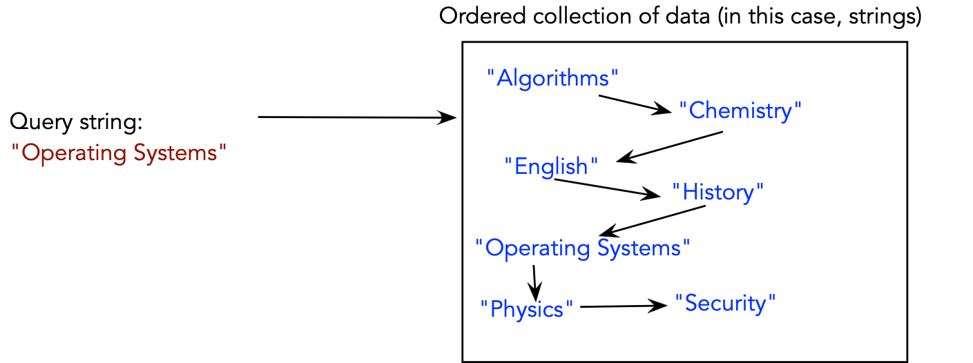
- Search:
Algorithm: search (key)
Input: a search key
1.   Initialize stack;
2.   found = false
3.   recursiveSearch (root, key)
4.   if found
5.     node = stack.pop()
6.     Extract value from node;
       // For insertions:
7.     stack.push (node)
8.     return value
9.   else
10.    return null
11.  endif
Output: value corresponding to key, if found.
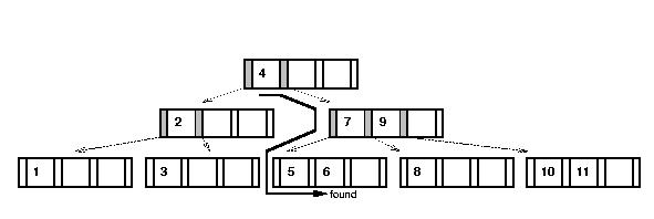
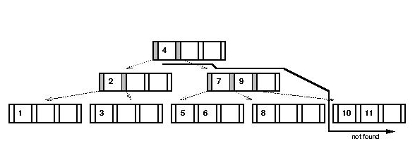
Algorithm: recursiveSearch (node, key)
Input: tree node, search key
1.   Find i such that i-th key in node is smallest key larger than or equal to key.
2.   stack.push (node)
3.   if found in node
4.     found = true
5.     return
6.   endif
     // If we're at a leaf, the key wasn't found.
7.   if node is a leaf
8.     return
9.   endif
     // Otherwise, follow pointer down to next level
10.  recursiveSearch (node.child[i], key)
- Insertion:
Algorithm: insert (key, value)
Input: key-value pair
1.   if tree is empty
2.     create new root and add key-value;
3.     return
4.   endif
     // Otherwise, search: stack contains path to leaf.
5.   search (key)
6.   if found
7.     Handle duplicates;
8.     return
9.   endif
10.  recursiveInsert (key, value, null, null)
Algorithm: recursiveInsert (key, value, left, right)
Input: key-value pair, left and right pointers
// First, get the node from the stack.
1. node = stack.pop()
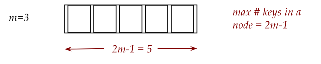
2. if node.numEntries < 2m-1
// Space available.
3. insert in correct position in node, along with left and right pointers.
4. return
5. endif
6. // Otherwise, a split is needed.
7. medianKey = m-th key in node;
8. medianValue = m-th value in node;
9. Create newRightNode;
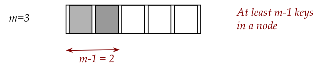
10. Place keys-values-pointers from 1,...,m-1 in current (left) node.
11. Place keys-values-pointers from m+1,...,2m-1 in newRightNode;
12. Put key and value in appropriate node (node or newRightNode).
13. if node == root
14. createNewRoot (medianKey, medianValue, node, newRightNode)
15. else
16. recursiveInsert (medianKey, medianValue, node, newRightNode)
17. endif
Recall the advantages of a multiway tree:
- The path length to any leaf is the same
⇒
the tree is always balanced
- This guarantees \(O(\log n)\) operations (search, insert).
But the disadvantages:
- If the nodes are mostly half-empty, that wastes space.
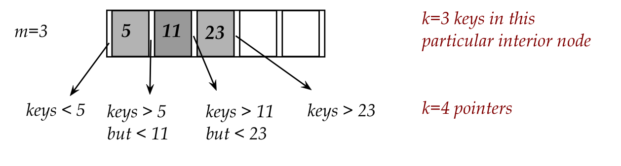
- There are two parts to searching:
- Finding the right node (tree search)
- Searching within a node
- We've lost the simplicity (search, insert) of the binary tree.
This raises the question: is there a hybrid between a multiway
tree and a binary tree?
The answer is yes, a red-black tree.
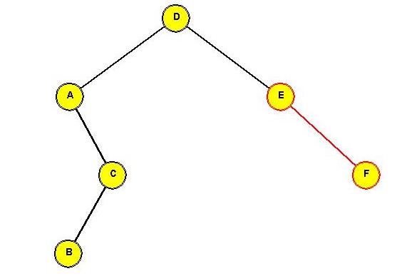
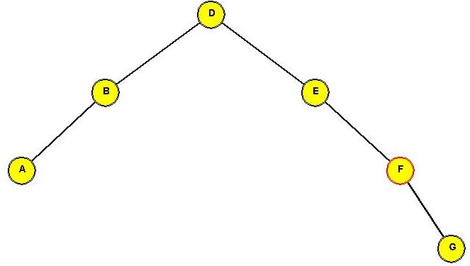
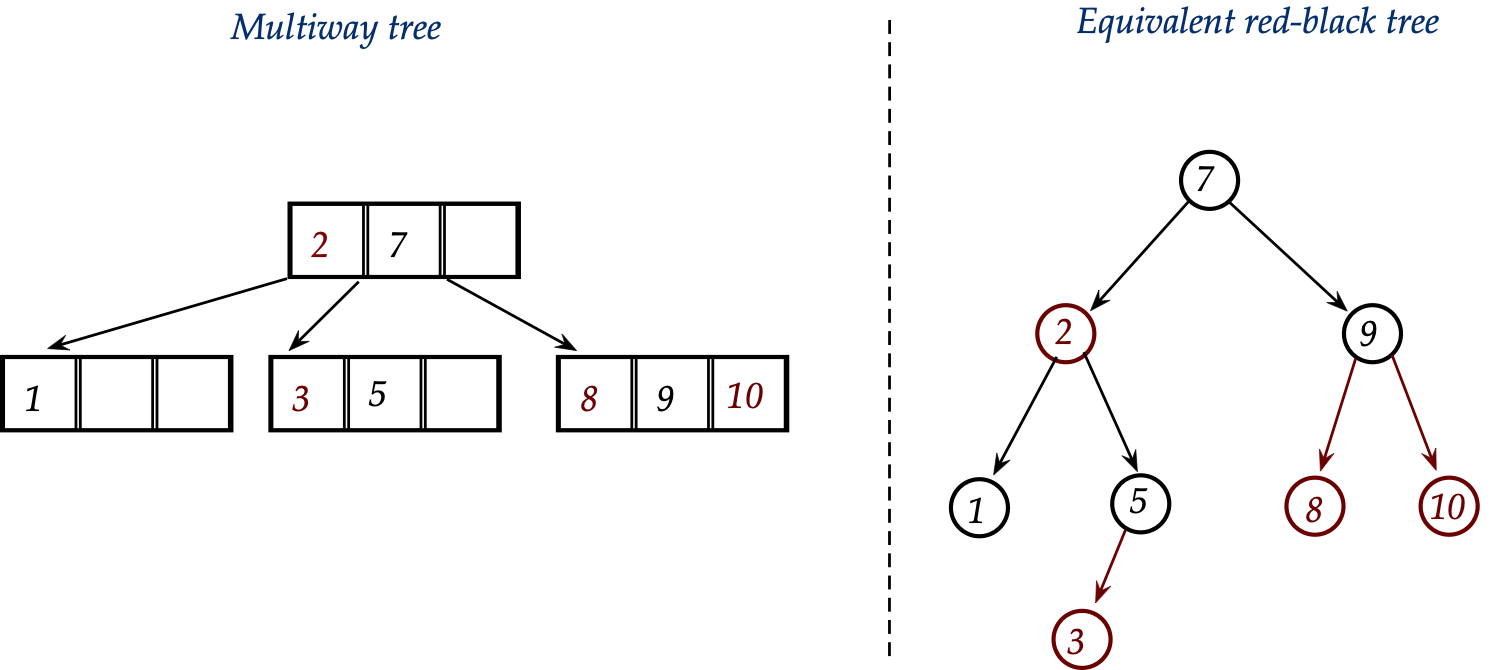
A red-black tree is really a binary-tree representation
of a multiway tree of degree 2:
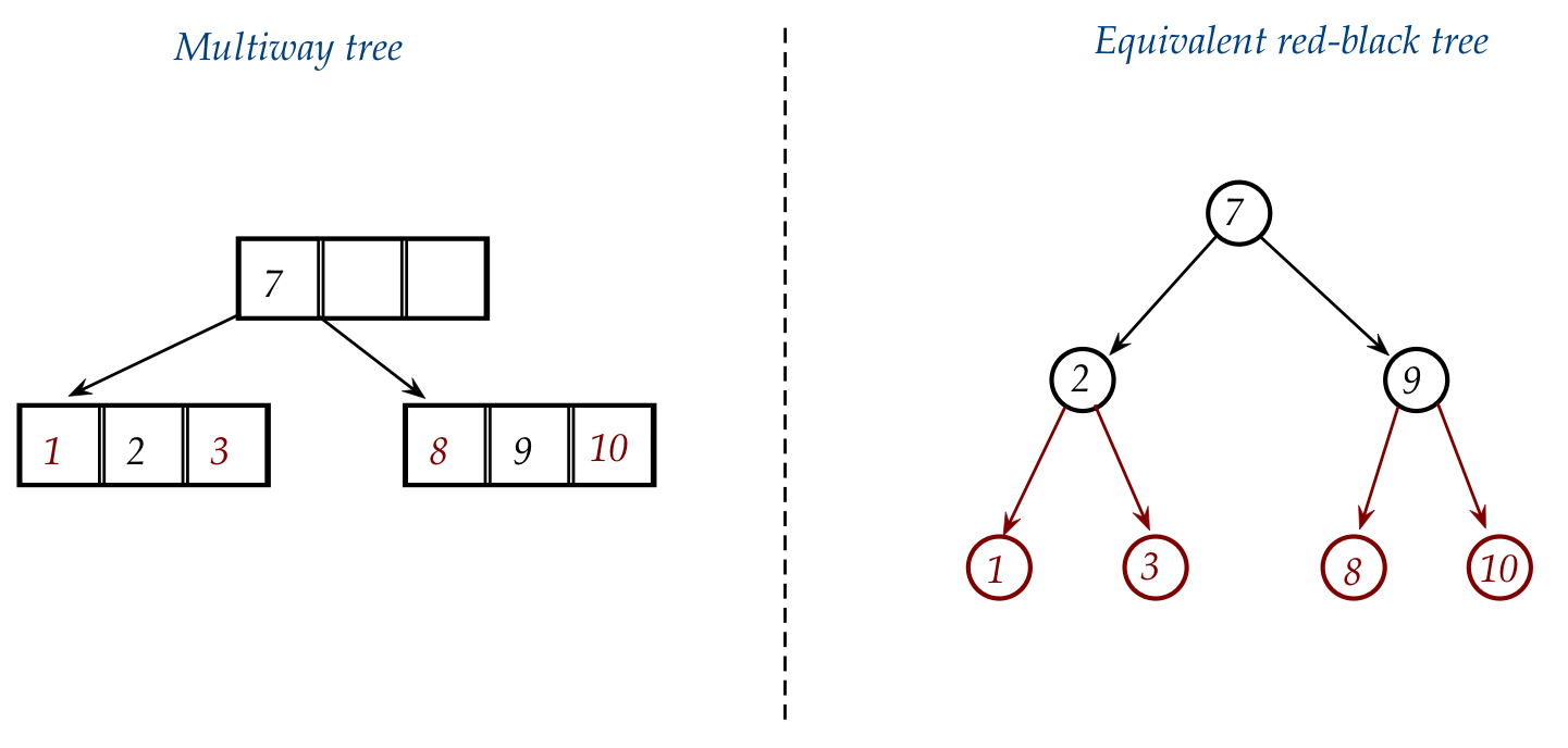
- A red-black tree is equivalent to a multiway tree of degree 2.
- But each node in a red-black tree is like a binary tree node
but with a color (red or black):
- Three pointers: left, right, parent.
- A color: red or black.
- Think of black nodes as representing the nodes
in the equivalent multiway tree.
- Think of red nodes as additional nodes needed when
values inside a multiway node are pulled out to become
binary tree nodes:
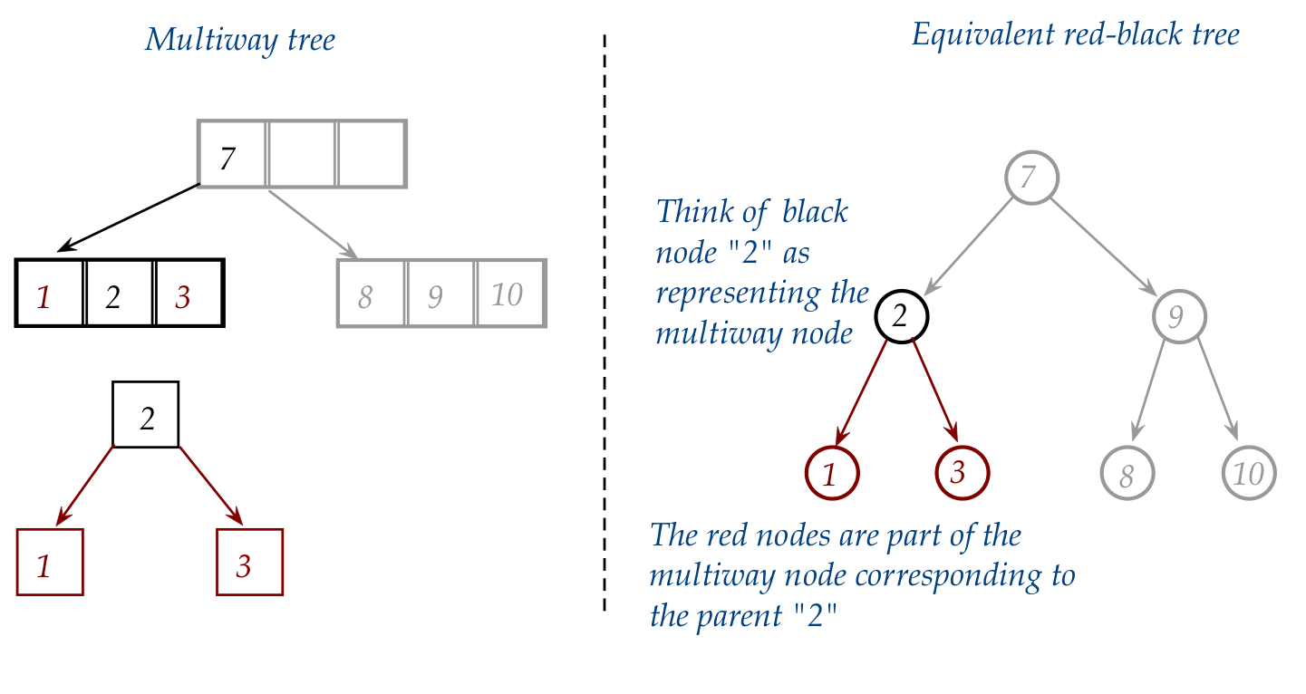
- The links are not colored, but we have drawn them so
because:
- A black node with one or two red children (and therefore red links)
should be thought of as one multiway node.
- It's as if the red links are elastic and can be retracted
to pull the red nodes into a glommed-together multiway node.
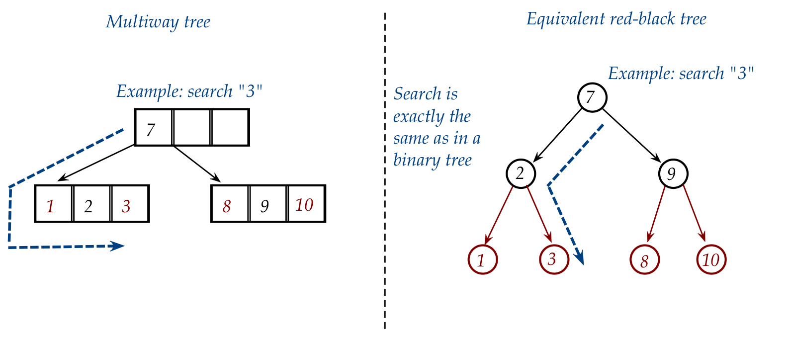
- Searching in a red-black tree is the same as in a
regular binary tree, in contrast to a multiway tree:
Insertion is the tricky operation, so let's take a closer look:
- We of course do not maintain a multiway tree and then
convert to red-black:
⇒
We're only showing them side-by-side for conceptual understanding
- Also, recall the easy and hard parts of insertion in
multiway tree:
- When it's easy: insertion occurs in a leaf node that already
has space.
- When it's hard: when the leaf node is full, and the node
is split, which can percolate up all the way to the root.
- Correspondingly, the two easy/hard cases for a red-black
tree are:
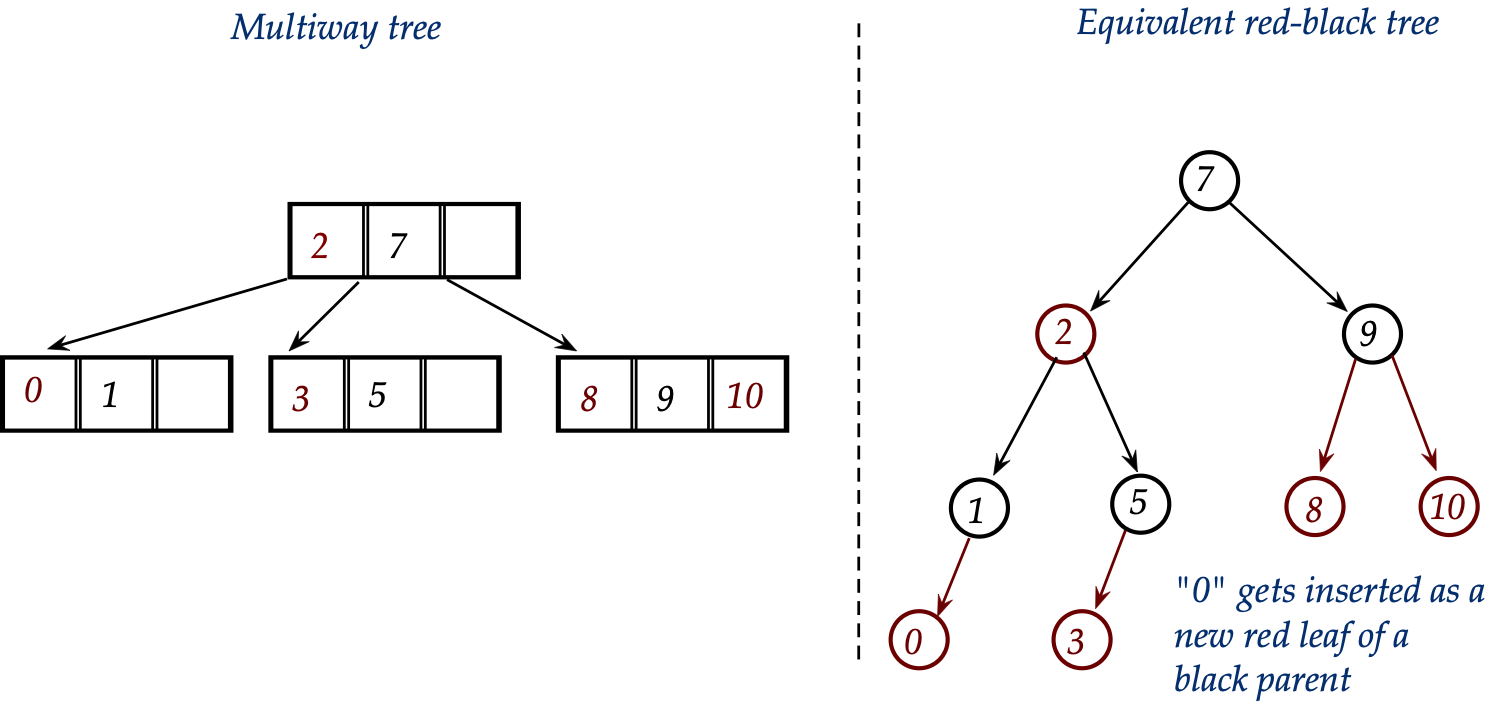
- Easy: when insertion occurs as a child of a black leaf.
- Hard: the other case.
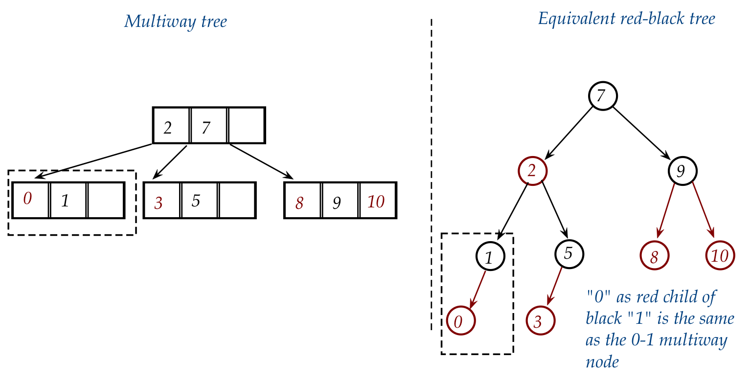
- An example of the easy case:
Consider inserting "0" into
- In the multiway equivalent, this is just plain insertion into
the leaf containing "1" but where "1" is now the center value:
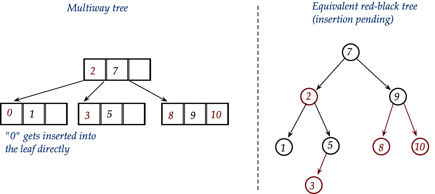
- In the red-black version:
- We'll do the hard case in two parts:
- When the multiway splits just once.
- When the multiway percolates up further towards the root.
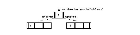
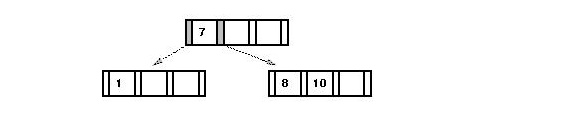
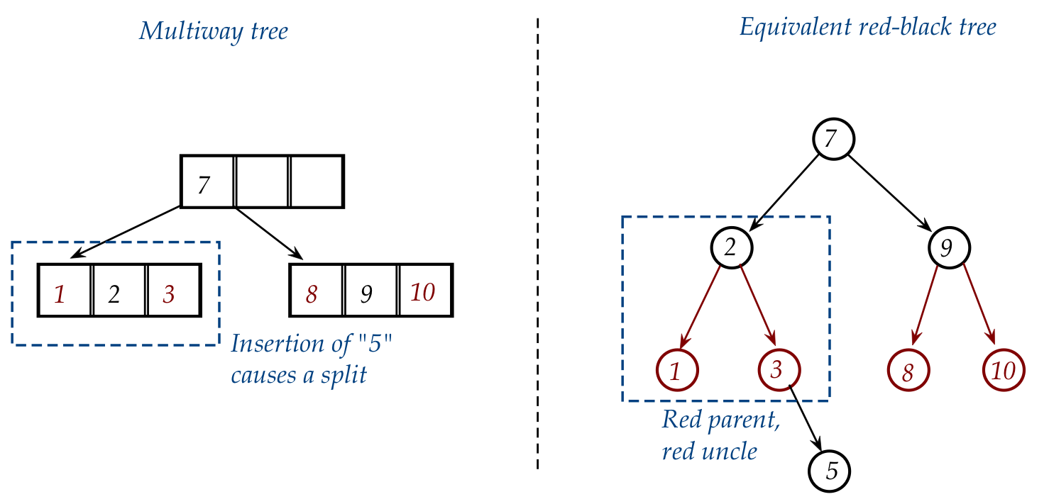
- Consider inserting "5" into

For the multiway tree:
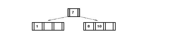
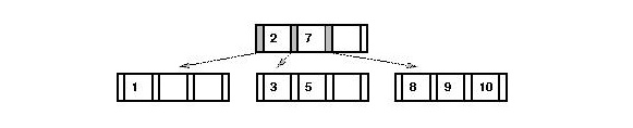
- We first need to split the "1-2-3" node and add "5" to the
right child:
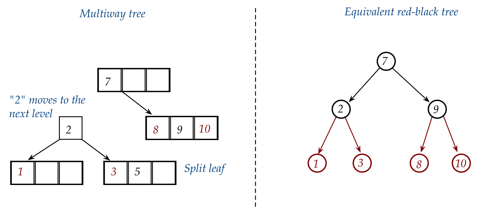
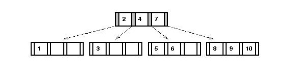
- Then "2" gets into the node above (which happens to be the
root here):
- What is the equivalent of "moving up" in the red-black tree?
⇒
A rotation!
(And, sometimes, a change of color)
- Let's follow the insertion of "5" into the equivalent
red-black tree:
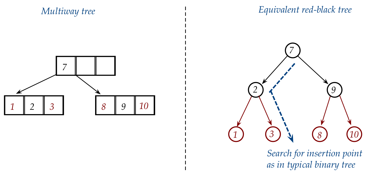
- After searching, we insert "5" as the right child of "3":

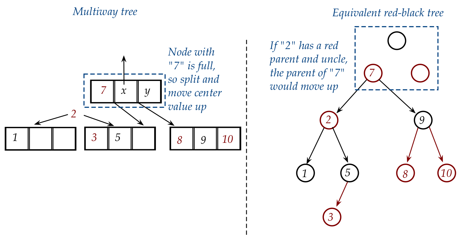
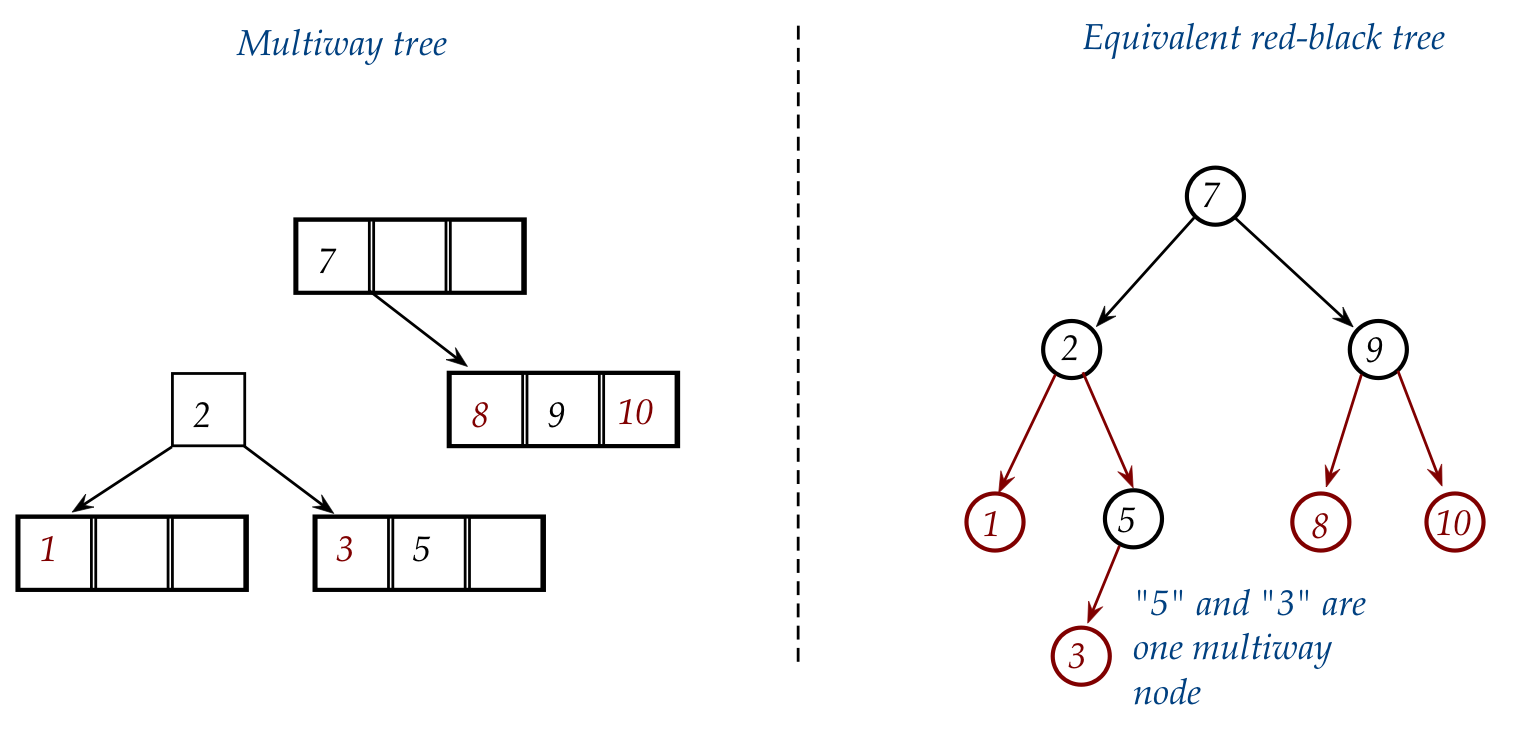
- Now consider what we did with the multiway: we split the
node containing "1-2-3".
- Here, "5" is the new center value of the equivalent multiway right-side node.
- Accordingly, to make "5" a center (black) value, we rotate
"5" into its parent's position in the red-black:

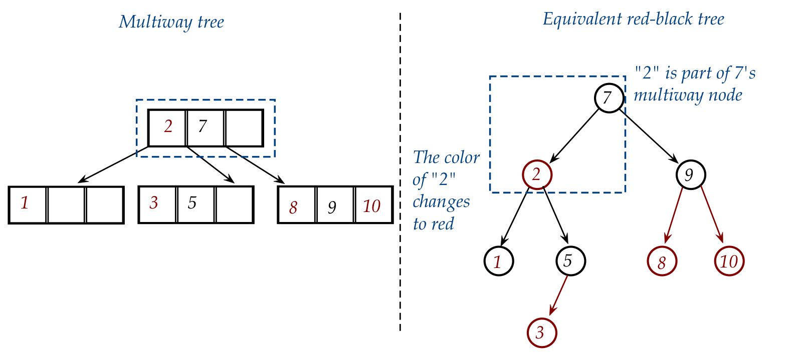
- This gives:
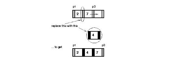
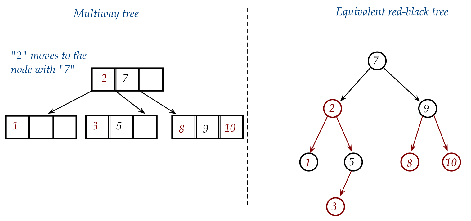
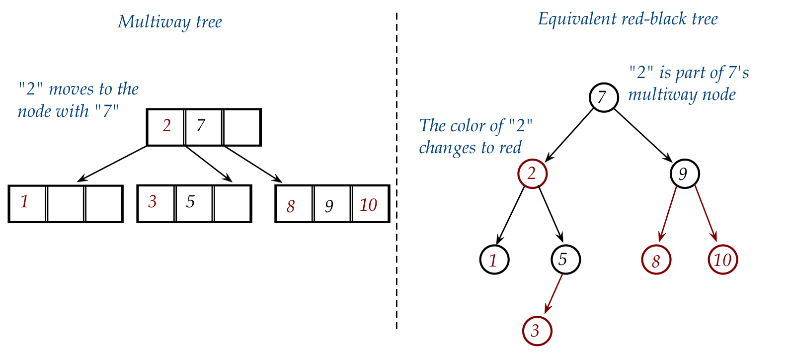
- Lastly, in the multiway tree, "2" moves into the node with "7".
- To make this happen in the red-black, we need to change the
color of "2" to red (to make it part of "7"):
Can we boil down the red-black cases into some simple "rules"?
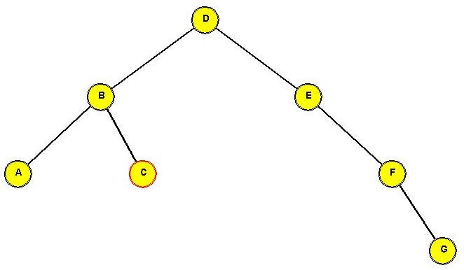
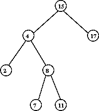
In-Class Exercise 3.9:
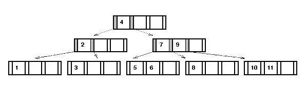
Draw the red-black tree corresponding to this multiway tree:
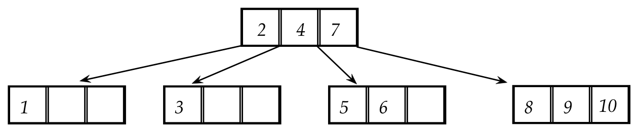
Then, insert the value "11" and, side-by-side, show the steps in both the
multiway tree and the red-black tree.
In-Class Exercise 3.10:
Argue that the number of black nodes counted along
a path from the root to any leaf is the same for all leaves.
Also, why is true that every red node must have a black parent?
Analysis:
- Since the number of black nodes along any path from root
to leaf is the same, the tree is balanced as far as black nodes
are concerned.
- Thus, the path length in terms of black nodes is
at most \(\log n\) for n keys in the tree.
- Each red node can lengthen the depth of a black node by at most 1.
- Thus, the worst path length is no more than \(2\log n\) .
- Search, which is a single walk down the tree,
therefore takes at most \(O(\log n)\).
- An insert operation includes a search, and can result
in rotations back up to the root, resulting in a constant
number of operations per rotation.
- Which means insert overall takes at most \(O(\log n)\).
3.6
Self-adjusting binary trees
What does "self-adjusting" mean?
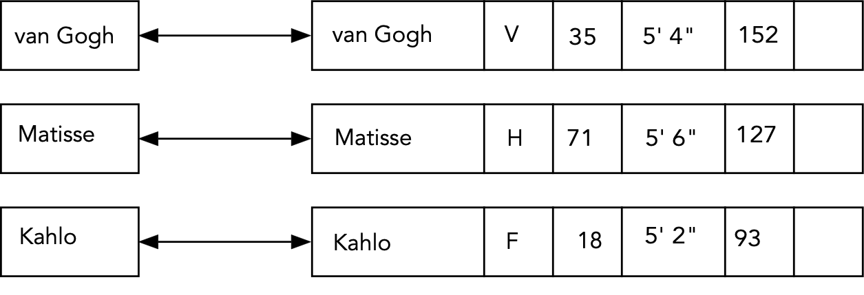
- Consider this linked list example:
- The list stores the 26 keys "A" ... "Z".
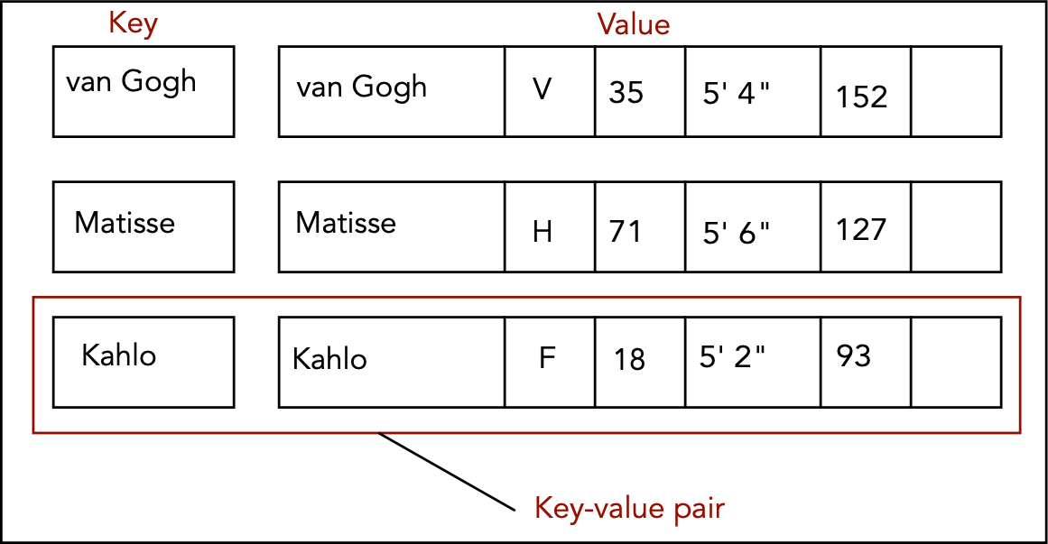
- For each letter, we store associated "value" information.
- Thus we have 26 key-value pairs.
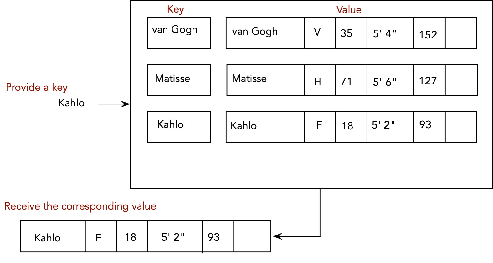
- Typical linked-list access:
- To access a particular key: start from the front and walk
down the list until the key is found.
- The time taken to find a particular key is the number of keys
before it in the list.
- Suppose we store the keys in the order "A" ... "Z":
- Is this the optimal order?
- What about the order "E" "T" "A" "I" "O" "N" ... ?
In-Class Exercise 3.11:
Suppose the frequency of access for letter "A" is
fA,
the frequency of access for letter "B" is
fB ... etc.
What is the best way to order the list?
- In many applications, the frequencies are not known.
- Yet: successive accesses provide some frequency information.
- Idea: why not re-organize the list with each access?
Self-adjusting linked lists:
- Move-To-Front strategy:
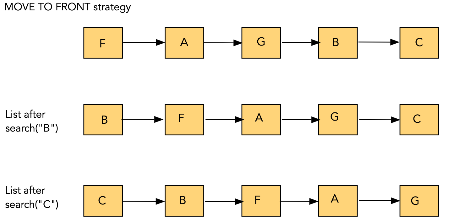
- Whenever an item is accessed, move the item to the front of the list.
- Cost of move: O(1) (constant).
- More frequently-accessed items will tend to be found towards
the front.
- Transpose strategy:
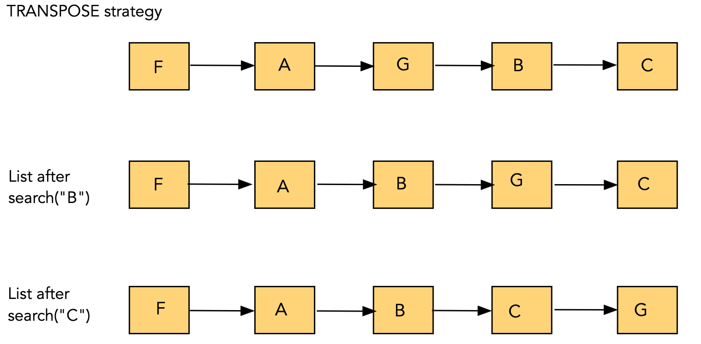
- Whenever an item is accessed, swap it with the one just ahead
of it
(i.e., move it towards the front one place)
- Cost of move: O(1).
- More frequently-accessed items will tend to bubble towards
the front.
In-Class Exercise 3.12:
Consider the following 5-element list with initial order: "A" "B" "C" "D" "E".
- For the Move-To-Front strategy with the access pattern "E" "E" "D" "E" "B" "E",
show the state of the list after each access.
- Do the same for the Transpose strategy with the above
access pattern.
- Create an access pattern that works well for Move-To-Front but
in which Transpose performs badly.
About self-adjusting linked lists:
- It can be shown that Transpose performs better than
Move-To-Front on average.
- It can be shown that no strategy can result in 50% lower
access costs than Move-To-Front.
- The analysis of self-adjusting linked lists initiated the area of
amortized analysis: analysis over a sequence of accesses (operations).
Self-adjusting binary trees:
- Where should frequently-accessed items be moved?
⇒ near the root.
- But ... re-arranging the tree might destroy the "in-order" property?
- To "move" an element towards the root: use rotations.
⇒ this keeps the "in-order" property intact.
Using simple rotations:
- A rotation can move a node into its parent's position.
- Goal: use successive rotations to move a node into root position.
- However:
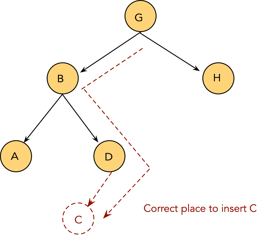
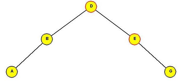
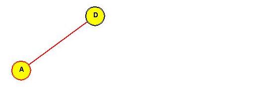
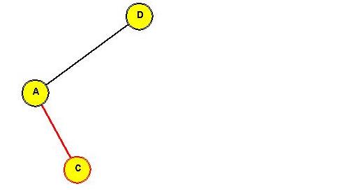
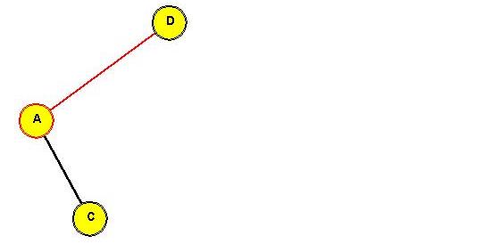
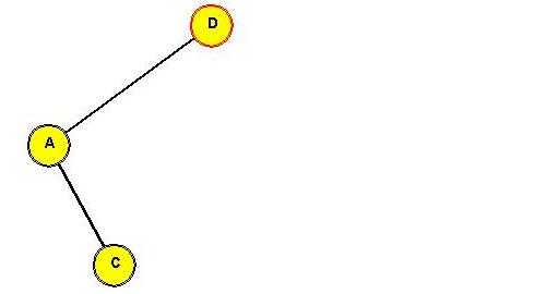
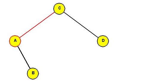
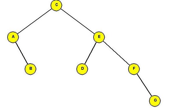
- Consider this example:
Tree before rotating "C" to the root:
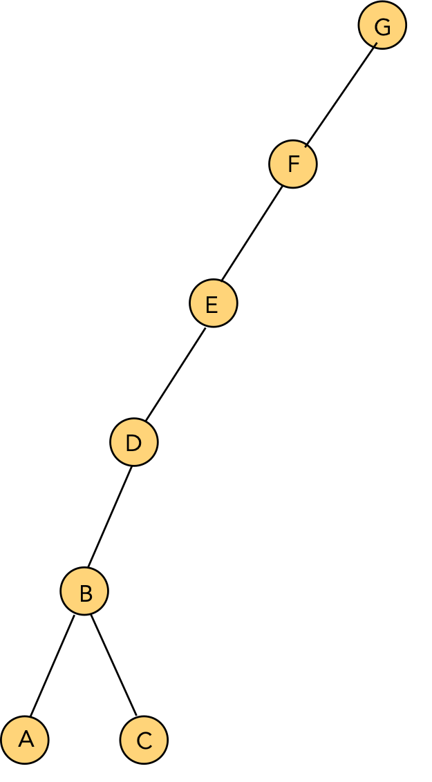
In-Class Exercise 3.13:
Show the intermediate trees obtained in rotating "C" to the root position.
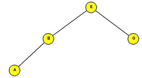
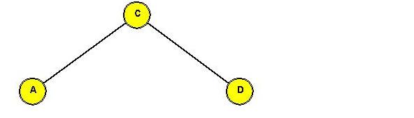
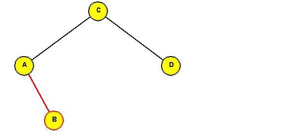
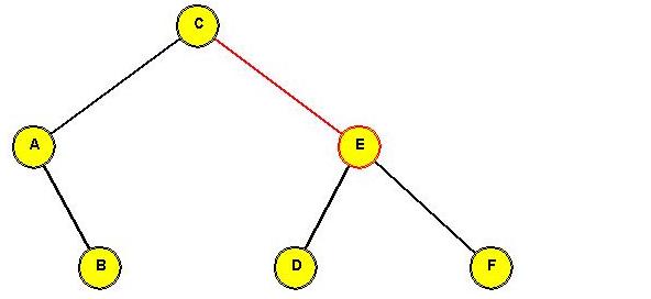
After rotating "C" to the root:
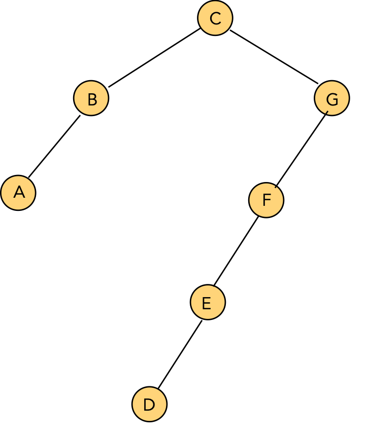
⇒ simple rotations can push "down one side".
- It can be shown that simple rotations can leave the tree unbalanced.
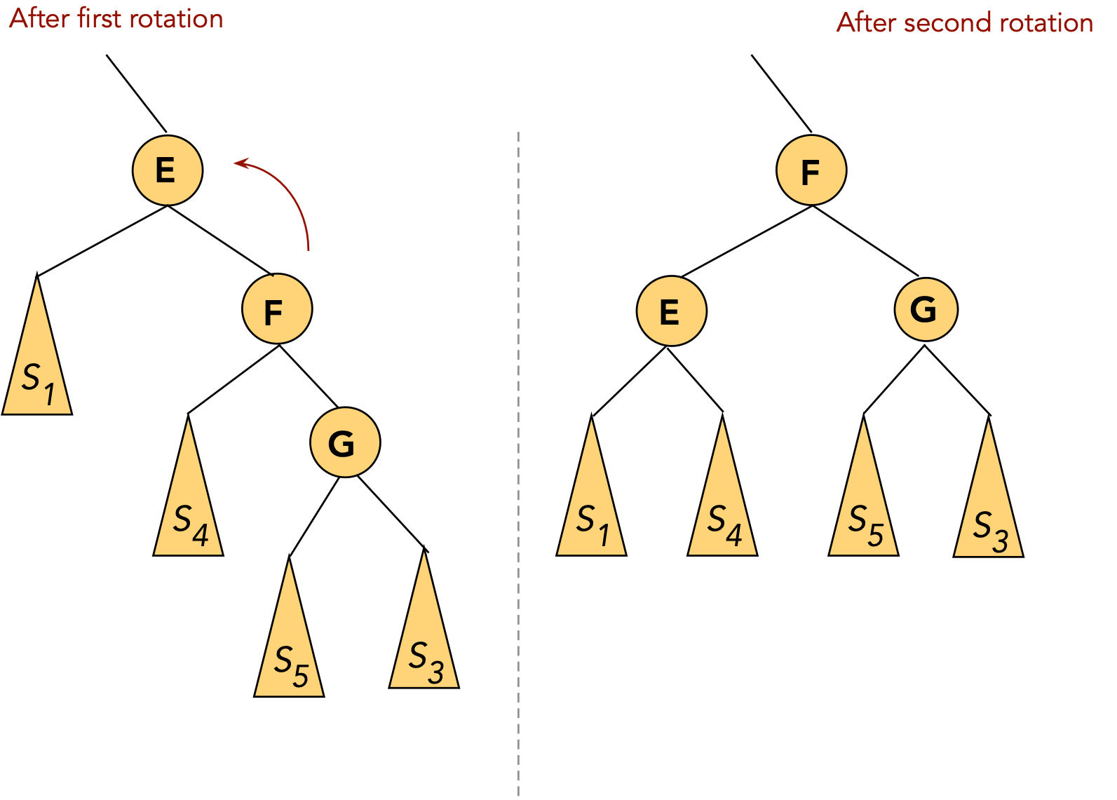
Using splaystep operations:
- The splaystep is similar to the AVL tree's double
rotation, but is a little more complicated.
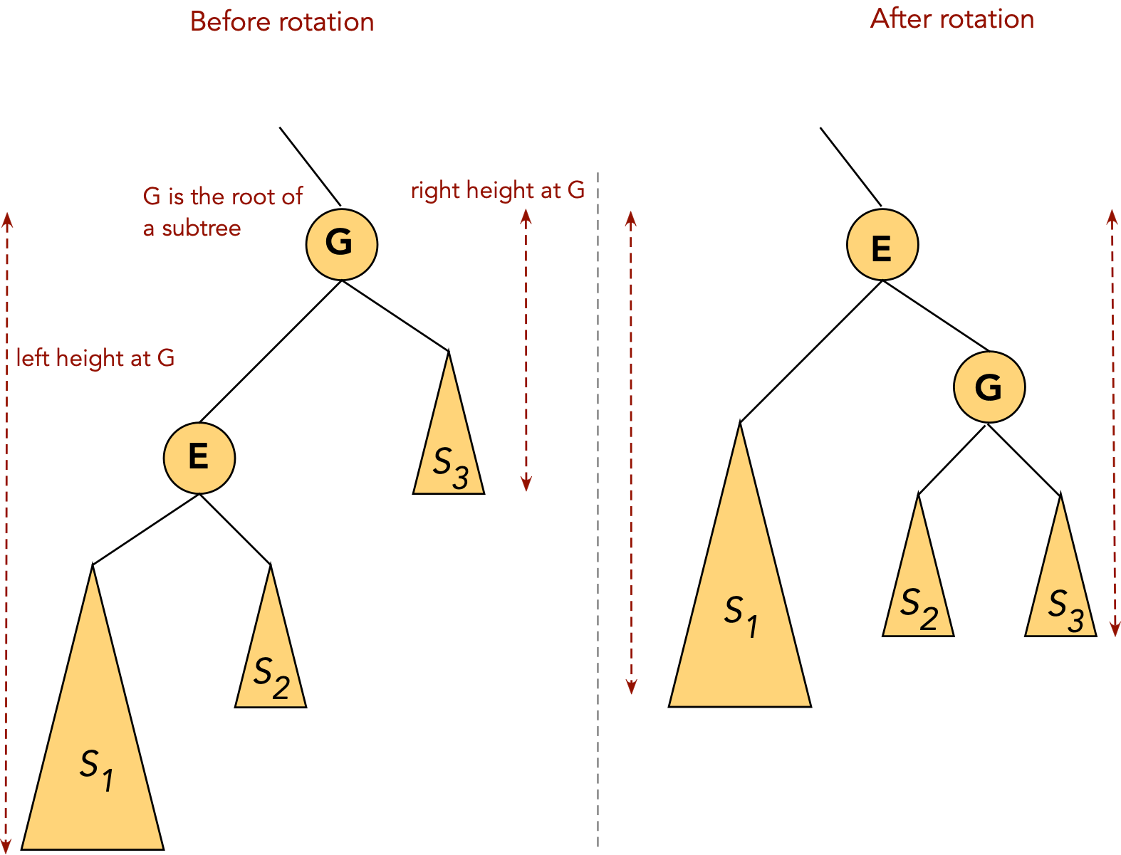
- Note: Below, \(S_1, S_2, ...\) etc
above refer to whole subtrees and
are not keys, whereas E and G are single nodes (keys).
- There are 5 cases:
- CASE 1: the target node (to move) is a child of the root.
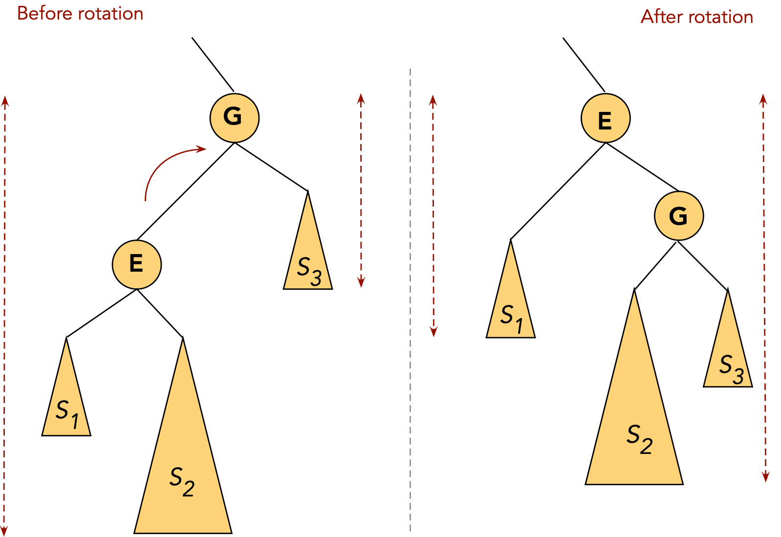
- CASE 1(a): target node (E, in this case) is the root's left child:
rotate node into root position.
⇒ rotate left child of root (in AVL terms).
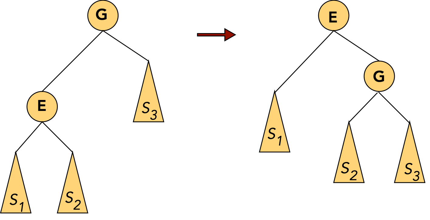
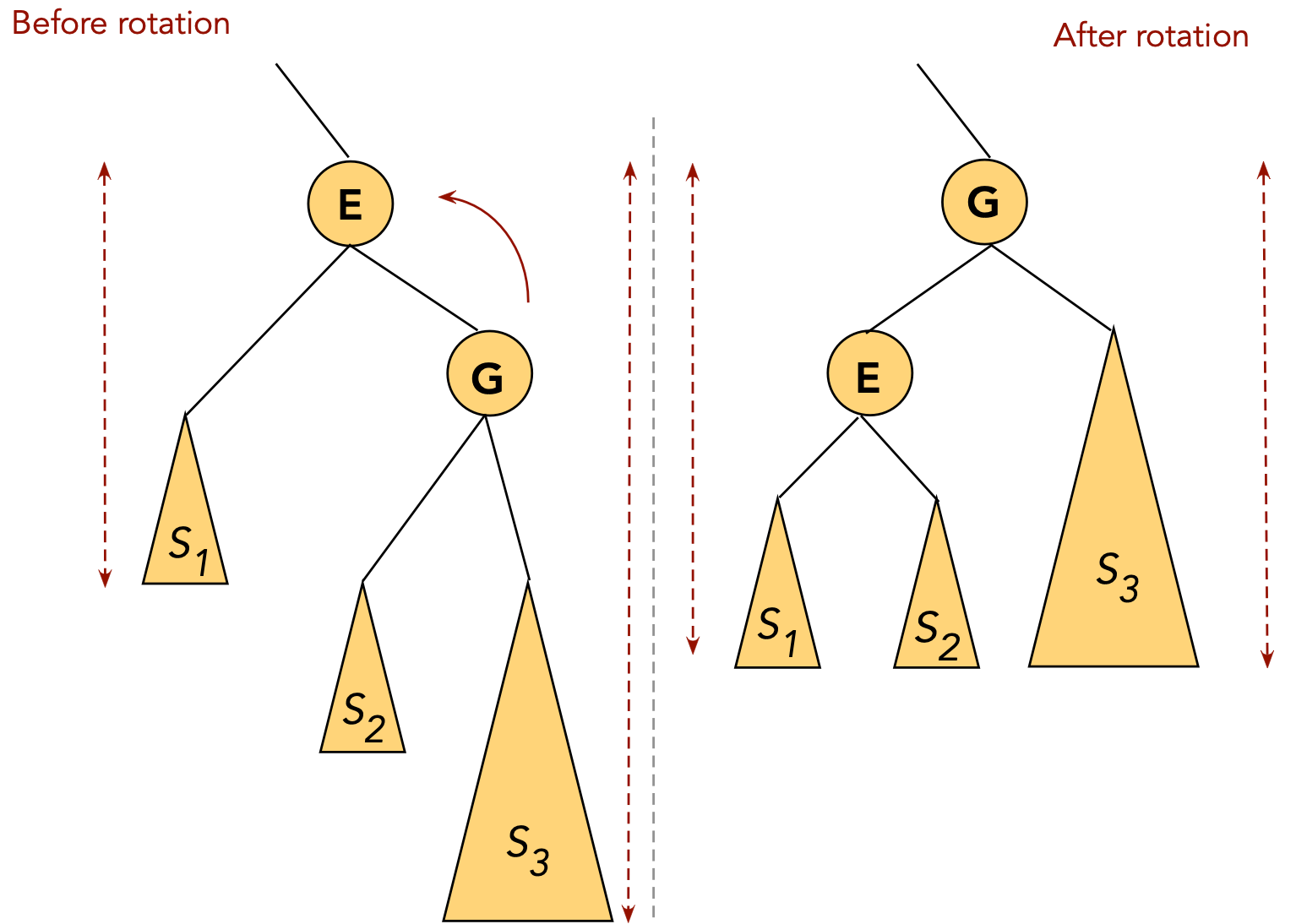
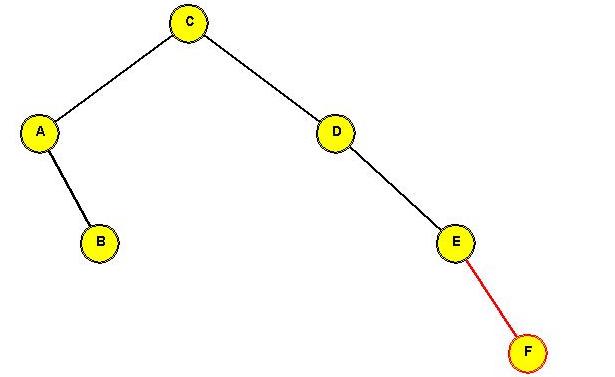
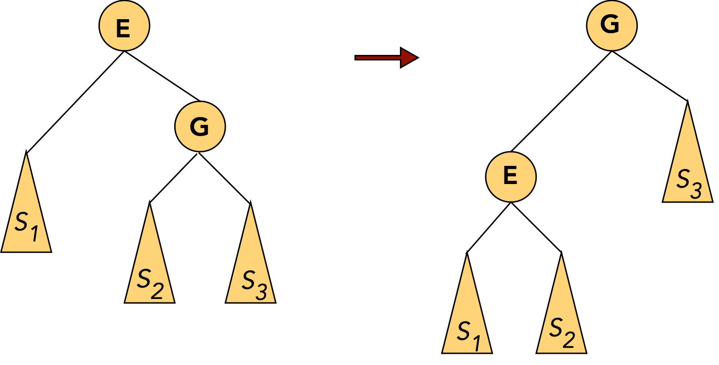
- CASE 1(b): target node (G, in this case) is the root's right child:
rotate node into root position.
⇒ rotate right child of root.
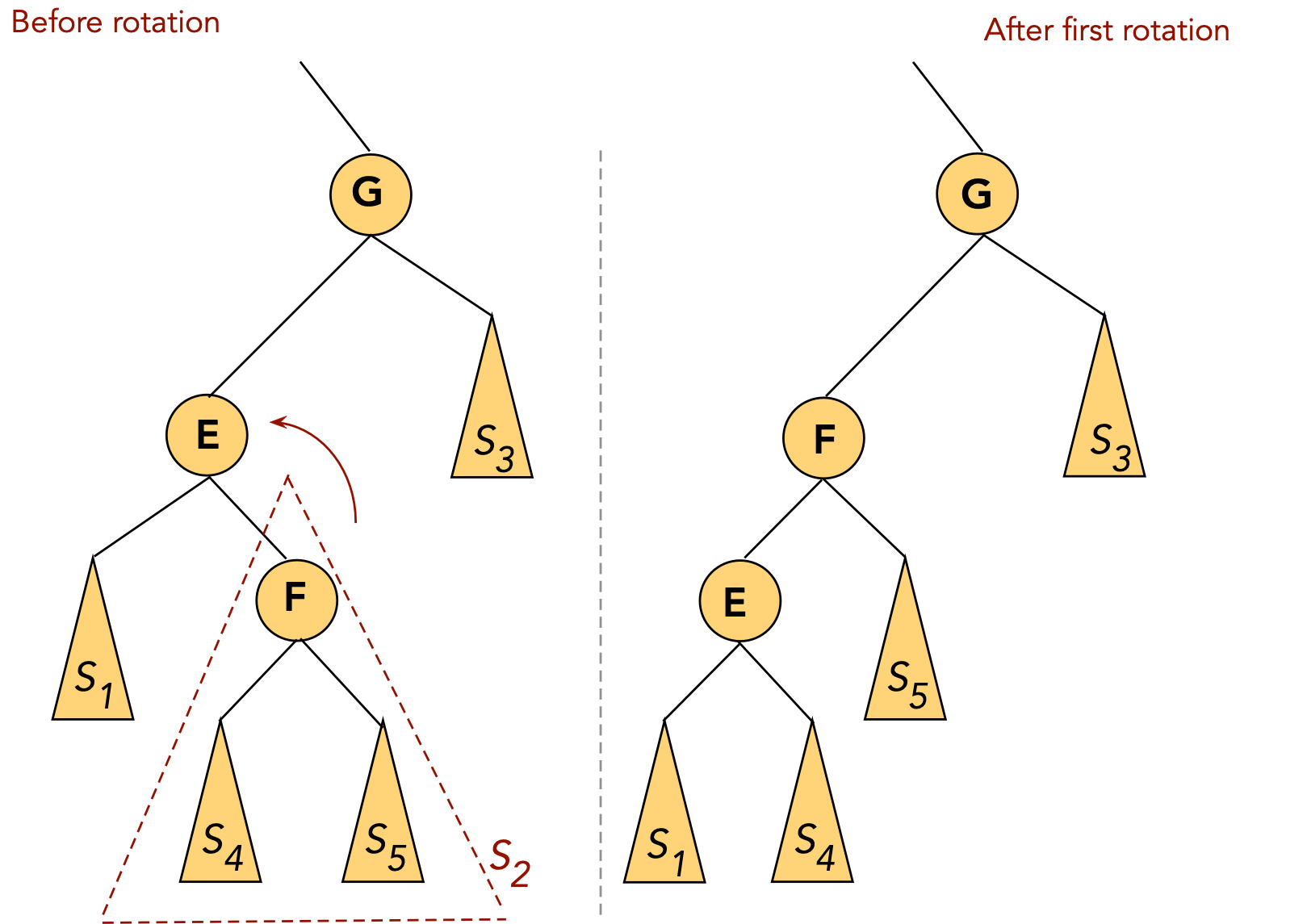
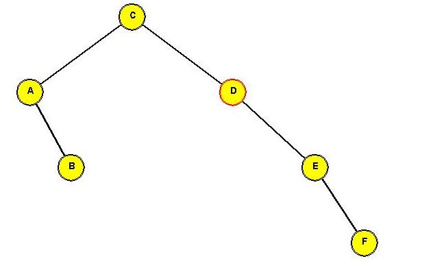
- CASE 2: the target (E) and the target's parent (G) are both left children
- First, rotate the parent into its parent's (grandparent's) position.
This will place the target at its parent's original level.
To do this: rotate the left child of the grandparent.
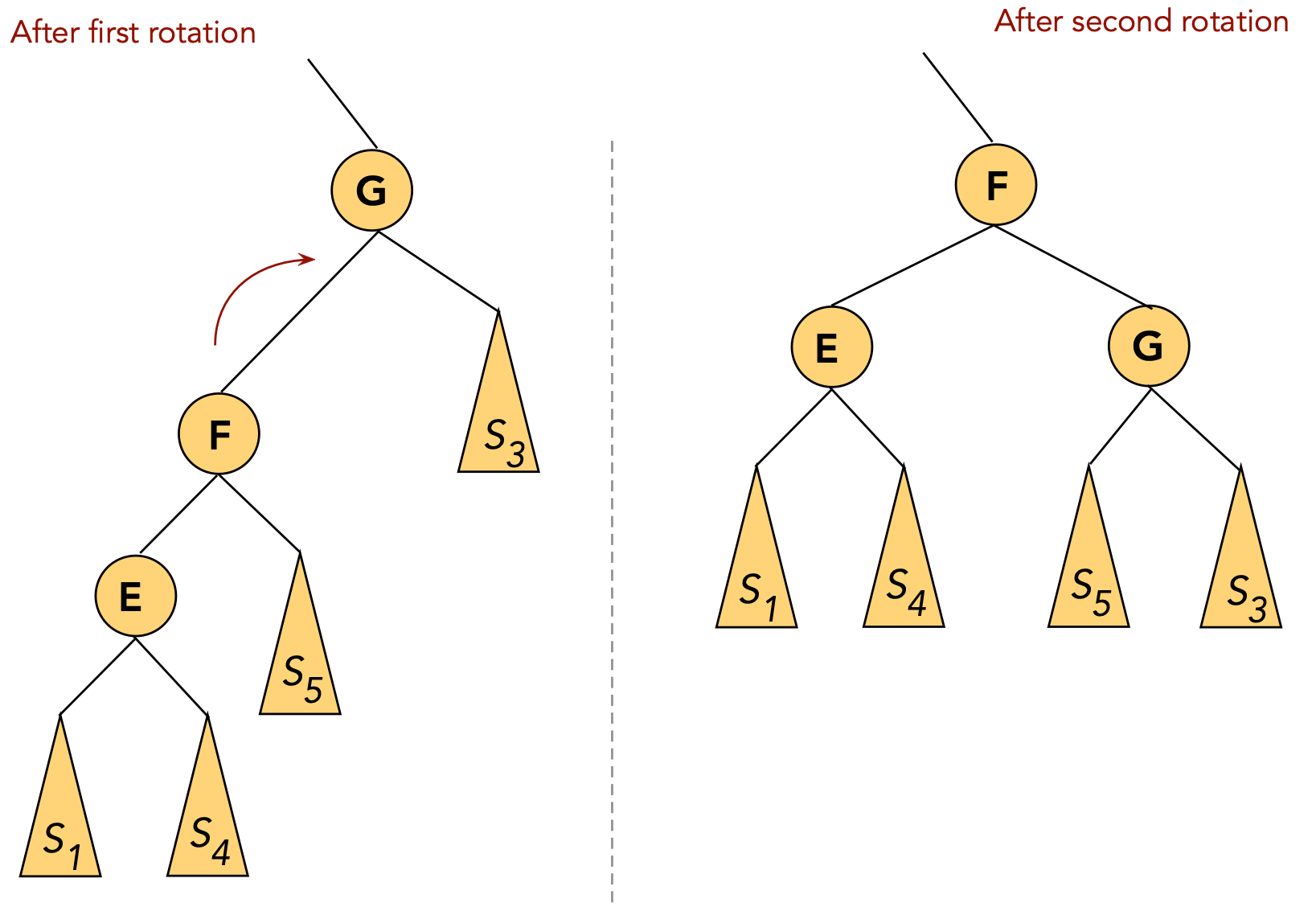
- Now rotate the target into the next level
This will place the target at its grandparent's original level.
To do this: rotate the left child of the parent
(which is now in the grandparent's old position)
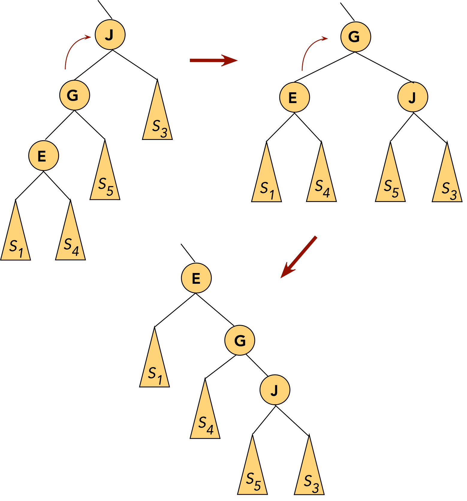
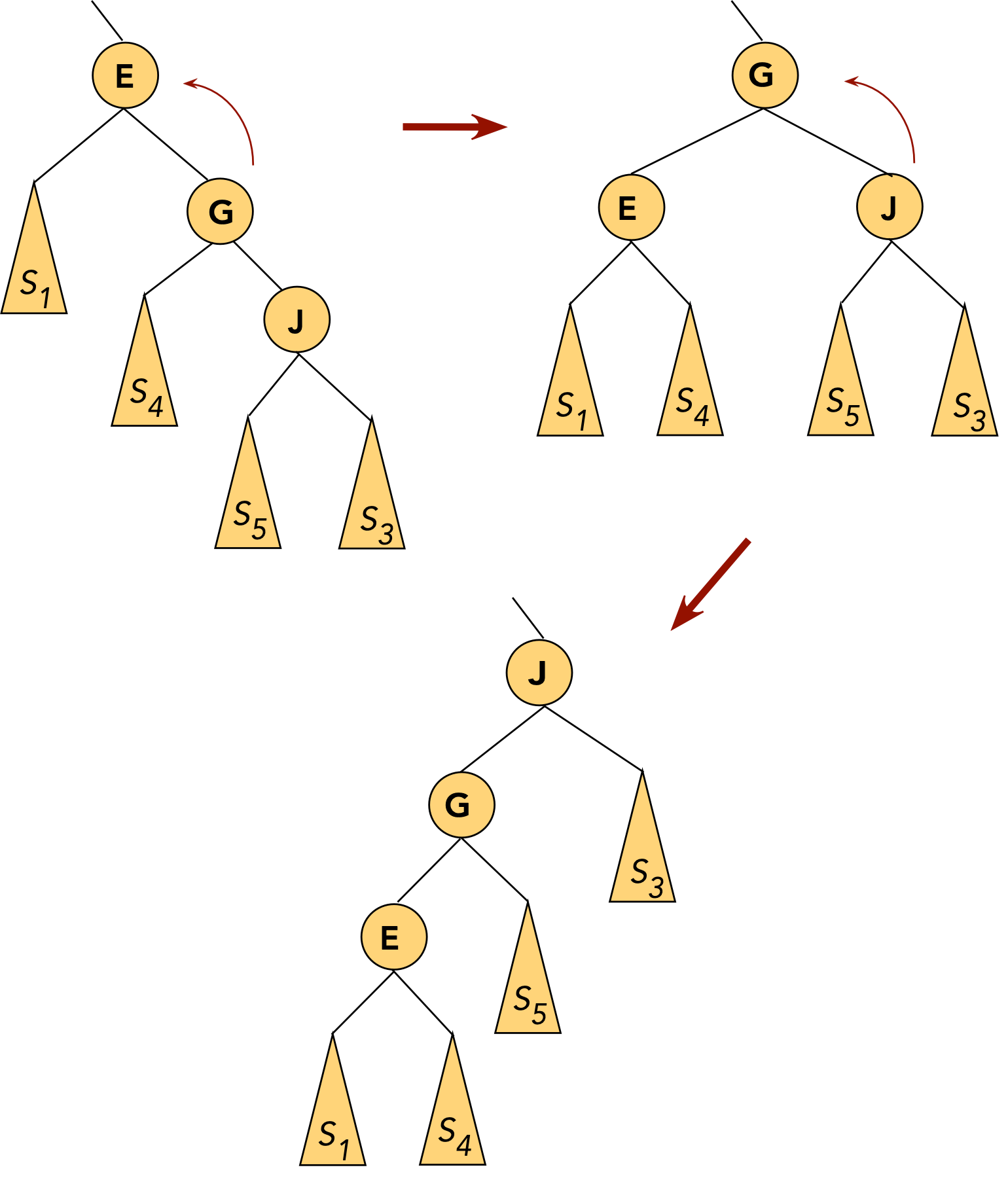
- CASE 3: the target (J) and the target's parent (G) are both right children
- First, rotate the parent into its parent's (grandparent's) position.
⇒ rotate the right child of the grandparent.
- Now rotate the target into the next level
⇒ rotate the right child of the parent
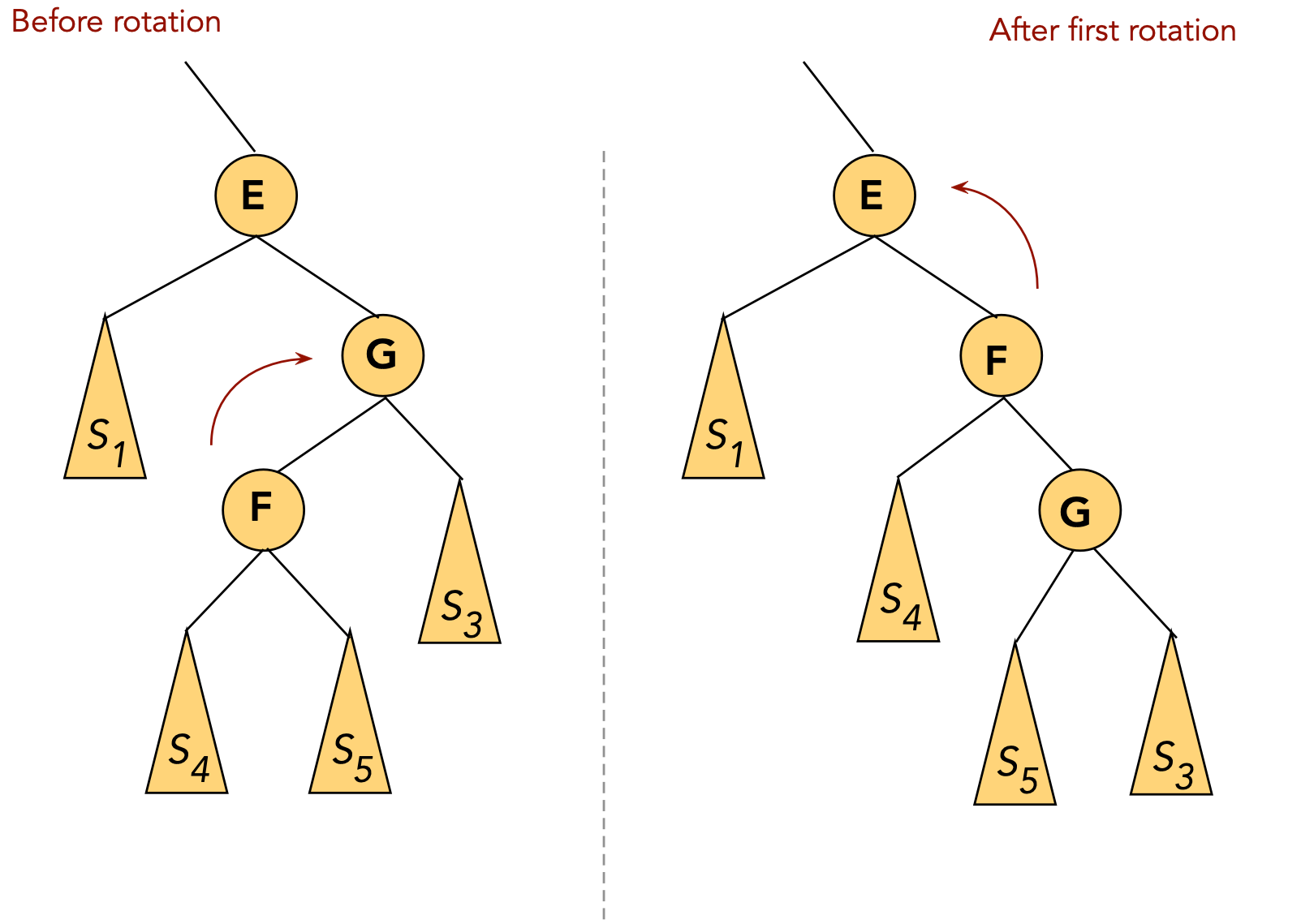
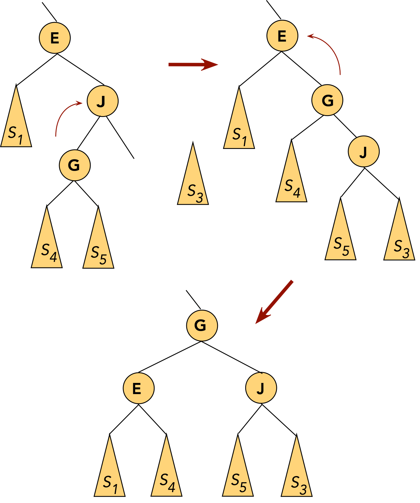
- CASE 4: the target (G) is a right child, the parent (E) is a left child.
- First, rotate the target into the parent's old position.
⇒ rotate the parent's right child.
- Now the target is a (left) child of the original grandparent.
- Next, rotate the target into the next level.
⇒ rotate left child of grandparent.
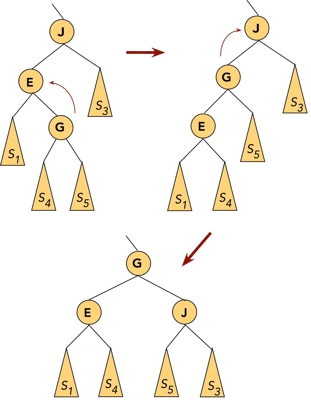
- CASE 5: the target (G) is a left child, the parent (J) is a right child.
- First, rotate the target into the parent's old position.
⇒ rotate the parent's left child.
- The target is now a (right) child of the original grandparent.
- Next, rotate the target into the next level.
⇒ rotate right child of grandparent.
- Thus, a target node may move up one or two levels in a
single splaystep operation.
- Through successive splaystep operations a target node can be
moved into the root position.
Search:
- Recursively traverse the tree, comparing with the input key, as in
binary search tree.
- If the key is found, move the target node (where the key was
found) to the root position using splaysteps.
- Pseudocode:
Algorithm: search (key)
Input: a search-key
1.   found = false;
2.   node = recursiveSearch (root, key)
3.   if found
4.     Move node to root-position using splaysteps;
5.     return value
6.   else
7.     return null
8.   endif
Output: value corresponding to key, if found.
Algorithm: recursiveSearch (node, key)
Input: tree node, search-key
1.   if key = node.key
2.     found = true
3.     return node
4.   endif
     // Otherwise, traverse further
5.   if key < node.key
6.     if node.left is null
7.       return node
8.     else
9.       return recursiveSearch (node.left, key)
10.    endif
11.  else
12.    if node.right is null
13.      return node
14.    else
15.      return recursiveSearch (node.right, key)
16.    endif
17.  endif
Output: pointer to node where found; if not found, pointer to node for insertion.
Insertion:
- Find the appropriate node to insert input key as a child, as in
a binary search tree.
- Once inserted, move the newly created node to the root
position using splaysteps.
- Pseudocode:
Algorithm: insert (key, value)
Input: a key-value pair
1.   if tree is empty
2.     Create new root and insert key-value pair;
3.     return
4.   endif
     // Otherwise, use search to find appropriate position
5.   node = recursiveSearch (root, key)
6.   if found
7.     Handle duplicates;
8.     return
9.   endif
     // Otherwise, node returned is correct place to insert.
10.  Create new tree-node and insert as child of node;
11.  Move newly created tree-node to root position using splaysteps;
Deletion:
- Same as in binary search tree.
Analysis:
- It is possible to show that occasionally the tree gets
unbalanced
⇒ particular operations may take O(n) time.
- Consider a sequence of m operations (among: insert,
search, delete).
- One can show: O(m log(n)) time for the m
operations overall.
- Thus, some operations may take long, but others will be short
⇒ amortized time is O(log(n)) per operation.
- Note: amortized O(log(n) time is stronger
(better) than statistically-average O(log(n) time.
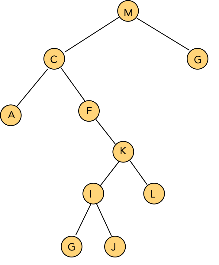
In-Class Exercise 3.14:
Show the intermediate trees and final tree after "J" is moved into the
root position using splaysteps. In each case, identify which "CASE" is
used.
Lastly, are there other kinds of useful "tree" data structures?
Yes. Some examples (not covered in this course):
- Binomial heap, skew heap (both as priority queues)
- kd-tree, R-tree, quadtree (all three for geometric data)