$ \newcommand{\eqb}[1]{\begin{eqnarray*}#1\end{eqnarray*}} \newcommand{\eqbn}[1]{\begin{eqnarray}#1\end{eqnarray}} \newcommand{\bb}[1]{\mathbf{#1}} \newcommand{\nchoose}[2]{\left(\begin{array}{c} #1 \\ #2 \end{array}\right)} \newcommand{\defn}{\stackrel{\vartriangle}{=}} \newcommand{\eql}{\;\; = \;\;} \definecolor{dkblue}{RGB}{0,0,120} \definecolor{dkred}{RGB}{120,0,0} \definecolor{dkgreen}{RGB}{0,120,0} \newcommand{\bigsp}{\;\;\;\;\;\;\;\;\;\;\;\;\;\;\;\;\;\;\;\;\;\;\;\;} \newcommand{\plss}{\;\;+\;\;} \newcommand{\miss}{\;\;-\;\;} \newcommand{\implies}{\Rightarrow\;\;\;\;\;\;\;\;\;\;\;\;} $

Module 9: Shortest Paths and Dynamic Programming

9.1 Single-Source Shortest Paths: Additional Topics

We will now consider three variations of the single-source shortest-path problem:

When edges have negative weights.
Directed graphs.
DAG's.

Negative weights:

Some applications require some edges to have negative weights.
Dijkstra's algorithm does not work with negative weights:
- Recall: once we extract a vertex v from the priority queue, it is never visited again.
  ⇒ if a negative-edge path to v is explored later, the algorithm does not record it.
- Even adding a large positive number to all edge weights (to make them positive) does not work. (Why?)
Negative weight cycles:
- On the left, the path from A to C is not affected by the positive weight cycle BDE.
- On the right, repeated traversals through BDE keep decreasing the path length from A to C
  ⇒ no solution possible.
Use the Bellman-Ford Algorithm for negative weights (see Cormen book):
- Variation of Dijkstra's algorithm.
- Takes O(VE) time.

Directed graphs:

Dijkstra's algorithm works (almost) without modification for directed graphs.
In exploring edges, we must ensure we are only exploring out-going edges:
If the graph representation is standard, this is already taken care of:
- Adjacency-matrix: non-zero entry indicates directed edge.
- Adjacency-list: only out-going edges are in a vertex list.

DAG's:

DAG's have additional structure (no cycles)
⇒ is a faster algorithm possible?
Recall: topological sort takes O(E) time.
Recall: in Dijkstra's algorithm, vertices are explored in "priority" order.
Note:
- In a DAG, exploring a "downstream" vertex cannot affect the shortest path to an upstream vertex.
- If the source is "downstream", no path is possible.
Key observation: exploring vertices in topological-sort order is sufficient.

Pseudocode:


Algorithm: DAG-SPT (G, s)
Input: Graph G=(V,E) with edge weights and designated source vertex s.

     // Initialize priorities and create empty SPT. 
1.   Set priority[i] = infinity for each vertex ;
     // Sort vertices in topological order and place in list. 
2.   vertexList = topological sort of vertices in G;
     // Place source in shortest path tree. 
3.   priority[s] = 0
4.   Add s to SPT;

     // Process remaining vertices. 
5.   while vertexList.notEmpty()
         // Extract next vertex in topological order. 
6.       v = extract next vertex in vertexList;
         // Explore edges from v. 
7.       for each neighbor u of v
8.           w = weight of edge (v, u);
             // If there's a better way to get to u (via v), then update. 
9.           if priority[u] > priority[v] + w
10.              priority[u] = priority[v] + w
11.              predecessor[u] = v
12.          endif
13.      endfor
14.  endwhile

15.  Build SPT;
16.  return SPT

Output: Shortest Path Tree (SPT) rooted at s.

Vertex-weighted DAG's:
- Consider the case where vertices have weights, but the edges don't, e.g.,
- To find shortest paths, apply a vertex's weight to each outgoing edge:
- Then solve as a regular DAG-SPT problem.

Longest path in a vertex-weighted DAG:

Application: vertices are tasks, weights are time-requirements.
Objective: find the earliest completion time for the whole set of tasks.
⇒ find the longest path.

Solution:

Transform into "task DAG" by adding source and sink vertices:
For each vertex, apply the vertex weight to each outgoing edge.
Use weight 0 on the source edges.

Use the "mirror image" (i.e., prefer larger weights) of the DAG-SPT algorithm above using the newly-added "source" as s.


Algorithm: maxWeightPath (G, s)
Input: Graph G=(V,E) with edge weights and designated source vertex s.

     // ... initialization same as DAG-SPT ... 

5.   while vertexList.notEmpty()
           // ... same as DAG-SPT ... 

           // Notice the reversal from ">" to "<": 
9.         if priority[u] < priority[v] + w
10.            priority[u] = priority[v] + w
               // ...  
12.        endif
14.  endwhile

     // ... same as DAG-SPT ... 
Output: Longest Path from source s.

The longest path is sometimes called the critical path in a task-graph.

9.2 All-Pairs Shortest Paths

The shortest-path between every pair of vertices:

Objective: find the shortest path between vertices i and j for every pair i and j.

One approach: run Dijkstra's algorithm using every vertex as a source:


Algorithm: Dijkstra-AllPairsShortestPaths (G)
Input: Graph G with edge weights.

1.   for each vertex i in G
       // Find the shortest path tree with i as source. 
2.     Dijkstra-SPT (i)
3.   endfor

4.   Construct paths;
5.   return paths

Output: shortest-path between each pair of vertices.

Running time: O(V E log(V))
For a dense graph, this becomes O(V³ log(V))
Note: path construction is omitted from the pseudocode above.

The Floyd-Warshall algorithm: takes O(V³) time.
⇒ uses an unusual approach.

Key ideas in the Floyd-Warshall algorithm:

Assume the n vertices are numbered 0, ..., n-1
Let S_k = { vertices 0, ..., k }.
Consider intermediate vertices on a path between i and j.
- Suppose we force ourselves to use intermediate vertices only from the set S_k = { 0, 1, 2, ..., k }.
- Note: i and j need not be in S_k.
- It is possible that no such path exists
  ⇒ path weight will be infinity.
Let D_ij^k = weight of shortest path from i to j using intermediate vertices in S_k.
Let w_ij = weight of edge ij.
We will let k = -1 define a "base case":
- Because k = -1, no intermediate vertices may be used.
  ⇒ D_ij^-1 = w_ij, if an edge from i to j exists.
- If we set w_ij = infinity when no edge is present,
  ⇒ D_ij^-1 = w_ij always.
Note:
- D_ij^k-1 = weight of shortest path from i to j using intermediate vertices in S_k-1 = { 0, 1, 2, ..., k-1 }.
Now, consider three cases:
- Case 1: k = -1
- Case 2: k >= 0 and vertex k is not in the D_ij^k path from i to j.
- Case 3: k >= 0 and vertex k is in the D_ij^k path from i to j.
Case 1: k = -1. Here, D_ij^-1 = w_ij (from before).
Case 2: vertex k is not in the path:
- In this case, the intermediate vertices are in S_k-1.
- Thus,
  D_ij^k = D_ij^k-1.
Case 3: vertex k is in the path:
- Consider the sub-paths not including k:
- By the containment property:
  - The path from i to k is the shortest path from i to k that uses intermediate vertices in S_k-1.
  - The path from k to j is the shortest path from k to j that uses intermediate vertices in S_k-1.
- Thus,
  D_ij^k = D_ik^k-1 + D_kj^k-1.
Since only these three cases are possible, one of them must be true.
⇒ when k >= 0, D_ij^k must be the lesser of the two values D_ij^k-1 and D_ik^k-1 + D_kj^k-1.
(Otherwise D_ij^k wouldn't be optimal).

Thus, combining the three cases:

D_ij^k

w_ij

min ( D_ij^k-1, D_ik^k-1 + D_kj^k-1 )

if k = -1

if k >= 0

Note:

The above equation is only an assertion of a property (it's not an algorithm).
The equation really says "optimality for size k" can be expressed in terms of "optimality for size k-1".
Recall D_ij^k = optimal cost of going from i to j using vertices in S_k.
⇒ the overall optimal cost of going from i to j is: D_ij^n-1 (for n vertices).
Thus, we need to compute D_ij^n-1.
But, this only gives the optimal cost (or weight)
⇒ we will address the problem of actually identifying the paths later.

In-Class Exercise 9.1: Write pseudocode to recursively compute D_ij^n-1. Start with FloydWarshallRec.java and:

Write a recursive version of the Floyd-Warshall algorithm. All you need to do is fill in the code to compute D_ij^n-1 recursively using the recursive definition of D_ij^n-1.

Count the number of times the recursive function is called (the main method has a test case).

Draw the test-case graph on paper and verify that the algorithm is producing the correct results.

Implementation:

At first, a recursive approach seems obvious.
We will use an iterative approach:
- First, compute D_ij^k for k=0 (i.e., D_ij⁰)
- Then, use that to compute D_ij¹.
- ...
- Finally, use D_ij^n-2 to compute D_ij^n-1.

Pseudocode:


Algorithm: floydWarshall (adjMatrix)
Input: Adjacency matrix representation: adjMatrix[i][j] = weight of
       edge (i,j), if an edge exists; adjMatrix[i][j]=0 otherwise.

      // Initialize the "base case" corresponding to k == -1. 
      // Note: we set the value to "infinity" when no edge exists. 
      // If we didn't, we would have to include a test in the main loop below. 
1.    for each i, j
2.        if adjMatrix[i][j] > 0
3.            D^-1[i][j] = adjMatrix[i][j]
4.        else
5.            D^-1[i][j] = infinity
6.        endif
7.    endfor

      // Start iterating over k. At each step, use the previously computed matrix. 
8.    for k=0 to numVertices-1

          // Compute D^k[i][j] for each i,j.
9.        for i=0 to numVertices-1
10.           for j=0 to numVertices-1
11.               if i != j 
                  // Use the relation between D^k and D^k-1 
12.                   if D^k-1[i][j] < D^k-1[i][k] + D^k-1[k][j]     // CASE 2
13.                       D^k[i][j] = D^k-1[i][j]
14.                   else
15.                       D^k[i][j] = D^k-1[i][k] + D^k-1[k][j]      // CASE 3
16.                   endif
17.               endif
18.           endfor
19.       endfor

        // Matrix copy: current D^k becomes next iteration's D^k-1 
20.     D^k-1 = D^k

21.   endfor

      // The D^k matrix only provides optimal costs. The 
      // paths still have to be built using D^k. 
22.   Build paths;
23.   return paths

Output: paths[i][j] = the shortest path from i to j.

Sample Java code (source file)

 
  public void allPairsShortestPaths (double[][] adjMatrix)
  {

    // Dk_minus_one = weights when k = -1 
    for (int i=0; i < numVertices; i++) {
      for (int j=0; j < numVertices; j++) {
        if (adjMatrix[i][j] > 0)
          Dk_minus_one[i][j] = adjMatrix[i][j];
        else 
          Dk_minus_one[i][j] = Double.MAX_VALUE;
        // NOTE: we have set the value to infinity and will exploit 
        // this to avoid a comparison. 
      }
    }
    

    // Now iterate over k. 

    for (int k=0; k < numVertices; k++) {

      // Compute Dk[i][j], for each i,j 

      for (int i=0; i < numVertices; i++) {
        for (int j=0; j < numVertices; j++) {
          if (i != j) {

            // D_k[i][j] = min ( D_k-1[i][j], D_k-1[i][k] + D_k-1[k][j]. 
            if (Dk_minus_one[i][j] < Dk_minus_one[i][k] + Dk_minus_one[k][j])
              Dk[i][j] = Dk_minus_one[i][j];
            else 
              Dk[i][j] = Dk_minus_one[i][k] + Dk_minus_one[k][j];

          }
        }
      }

      // Now store current Dk into D_k-1 
      for (int i=0; i < numVertices; i++) {
        for (int j=0; j < numVertices; j++) {
          Dk_minus_one[i][j] = Dk[i][j];
        }
      }

    } // end-outermost-for 


    // Next, build the paths by doing this once for each source. 

    // ... (not shown) ... 

  }

Analysis:

The triple for-loop says it all: O(V³).

In-Class Exercise 9.2: In FloydWarshall.java (the sample code above), count the number of times the innermost if-statement is executed. Explain the difference between this count and the one from the previous exercise: why is the earlier one so much higher?

An optimization:

Consider D_ik^k-1
D_ik^k-1 = optimal cost from i to k using S_k-1.
Observe: k cannot be an intermediate vertex in an optimal path that ends at k
⇒ cost does not change if we allow k to be an intermediate vertex.
⇒ D_ik^k-1 = D_ik^k.
Similarly, D_kj^k-1 = D_kj^k.
Thus, whether we use D_ik^k-1 or D_ik^k makes no difference.
⇒ we can use the updated matrix D_ik^k in loop.
⇒ only one matrix is needed!
One more observation: at the time of computing D_ij^k, the current "best value" is D_ij^k-1.

Thus, in the pseudocode, we can replace


12.           if D^k-1[i][j] < D^k-1[i][k] + D^k-1[k][j]
13.               D^k[i][j] = D^k-1[i][j]
14.           else
15.               D^k[i][j] = D^k-1[i][k] + D^k-1[k][j]
16.           endif

with


              // The first D^k[i][j] is really D^k-1[i][j] 
              // because we haven't written into it yet. 
12.           if D^k[i][j] < D^k[i][k] + D^k[k][j]
                  // This is superfluous: 
13.               D^k[i][j] = D^k[i][j]
14.           else
                  // This is all we need: 
15.               D^k[i][j] = D^k[i][k] + D^k[k][j]
16.           endif

We will now use a single matrix D[i][j]:


Algorithm: floydWarshallOpt (adjMatrix)
Input: Adjacency matrix representation: adjMatrix[i][j] = weight of
       edge (i,j), if an edge exists; adjMatrix[i][j]=0 otherwise.

      // ... initialization similar to that in floydWarshall ... 

1.    for k=0 to numVertices-1

2.        for i=0 to numVertices-1
3.            for j=0 to numVertices-1
4.                if i != j 
                      // Use the same matrix. 
5.                    if D[i][k] + D[k][j] < D[i][j] 
6.                        D[i][j] = D[i][k] + D[k][j]
7.                    endif
8.                endif
9.            endfor
10.       endfor

11.   endfor

      // ... path construction ...

9.3 Distributed Routing in a Network

Consider an alternative iterative version of Floyd-Warshall:

Recall the basic structure of the earlier Floyd-Warshall iteration:


    for k=0 to numVertices-1

        for each i,j
            Compute D^k_ij
        endfor

    endfor

What if we were to change to loop order to:
```
    for each i,j

        for k=0 to numVertices-1
            Compute D^k_ij
        endfor

    endfor
  
```
Would this work?
- Consider a particular i and j, e.g., 3 and 7.
- Once D[3][7] is computed, we never return to it again.
- Suppose D[4][5] (computed later) affects D[3][7]
  ⇒ we won't modify D[3][7] (as we should).
- On the other hand, if no other D[i][j] changes, then D[3][7] is correctly computed.

So, one needs to re-compute if a change occurred:


    while changeOccurred
        changeOccurred = false

        for each i,j

            for k=0 to numVertices-1
                // Compute D^k_ij
                if D[i][k] + D[k][j] < D[i][j] 
                    // Improved shortest-cost. 
                    D[i][j] = D[i][k] + D[k][j]
                    // Since this may propagate, we have to continue iteration. 
                    changeOccurred = true
                endif
            endfor

        endfor

    endwhile

Here is the more complete pseudocode: (source file)


Algorithm: floydWarshallIterative (adjMatrix)
Input: Adjacency matrix representation: adjMatrix[i][j] = weight of
       edge (i,j), if an edge exists; adjMatrix[i][j]=0 otherwise.

      // ... initialization similar to that in floydWarshallOpt ... 

1.    changeOccurred = true
2.    while changeOccurred

          changeOccurred = false

3.        for i=0 to numVertices-1
4.            for j=0 to numVertices-1
5.                if i != j 
                      // "k" is now in the innermost loop. 
6.                    for k=0 to numVertices
7.                        if D[i][k] + D[k][j] < D[i][j] 
                              // Improved shortest-cost. 
8.                            D[i][j] = D[i][k] + D[k][j]
                              // Since this may propagate, we have to continue iteration. 
9.                            changeOccurred = true
10.                       endif
11.                   endfor
10.               endif
11.           endfor
12.       endfor

13.   endwhile
      // ... path construction ...

This does not seem more efficient (it is not), but it's a useful observation for distributed routing.

What do we mean by "distributed routing"?

A "network" is a collection of computers connected together in some fashion (with links)
⇒ can represent a network using a graph.
Example: internet routers connected by links.
A "routing algorithm" provides for data to get sent across the network.
Centralized vs. Distributed:
- Routes can be computed centrally by a server.
- Or in a distributed fashion by routers (since routers are also, typically, computers).
Routes are computed frequently (e.g., as often as 30 milliseconds)
⇒ need an efficient way to computed routes.

In-Class Exercise 9.3: Why aren't routes computed just once and for all whenever a network is initialized?

Distributed Floyd-Warshall: a purely distibuted algorithm

Consider a different way of viewing the iterative version:


    while changeOccurred
        changeOccurred = false

        for i=0 to numVertices-1
            for j=0 to numVertices-1

            // Node i says "let me try to get to destination j via k". 
            for k=0 to numVertices
                // If it's cheaper for me to go via k, let me record that. 
                if D[i][k] + D[k][j] < D[i][j] 
                    // Improved shortest-cost: my cost to neighbor k, plus k's cost to j 
                    D[i][j] = D[i][k] + D[k][j]
                    changeOccurred = true
                endif

            endfor
         endfor

   endwhile

Key ideas:
- Each node maintains its current shortest-cost to each destination.
- Thus, node i maintains the value D_i[j] = "current best cost to get to destination j".
- Node i polls its neighbors asking them "how much does it cost you to get to j?".
- Node i uses these replies (and its own costs to get to neighbors) to find the best path.
- This process is repeated as long as changes propagate.
Example:
- We will show computations when node "5" is the destination.
  ⇒ in practice, the computation for all destinations occurs simultaneously.
- Each node maintains:
  - Its currently-known cost to get to "5",
  - Which neighbor is used in getting to "5"
  Initially, nothing is known:
- After the first round of message-exchange between neighbors:
- After the next round:
- After the next round:
- The next round reveals no changes
  ⇒ algorithm halts (nodes stop exchanging information).

An alternative: running Dijkstra at each node

All nodes acquire complete information about the network
⇒ topology and edge weights.
Each node runs Dijkstra's algorithm with itself as root.
⇒ each node know which outgoing link to use to send data (to a particular destination).
How is edge-information exchanged?
- Use a broadcast or flooding algorithm (separate topic).
We might call this a semi-distributed algorithm.
⇒ All nodes perform the same computation.

The process of "routing":

How is a packet of data routed?

Each node maintains a routing table
e.g., the table at node 0 in the earlier example

Destination	Current cost	Outgoing link
...	...	...
...	...	...
5	4	(0,2)
...	...	...

When a packet comes in, the destination written in the packet is "looked up" in the table to find the next link.
Destination-based routing:
- The routing table is indexed only by destination.
- This is because of the "containment" property of shortest-path routing.
- Example: (above) whenever a packet for 5 comes into node 0, it always goes out on link (0, 2).
  ⇒ it doesn't matter where the packet came from.
Destination-based routing is simpler to implement.

Alternative: routing based on both source and destination.
⇒ requires more space.

Source	Destination	Current cost	Outgoing link
...	...	...	...
...	...	...	...
1	5	x	(0,2)
...	...	...	...
0	5	y	(0,3)
...	...	...	...

Internet routing:

The old internet (up to mid-80's) used a version of distributed-Floyd-Warshall.
⇒ called RIP (Routing Information Protocol).
RIP has problems with looping.
⇒ mostly discontinued (but still used in places).
The current protocol (called OSPF) uses the semi-distributed Dijkstra's algorithm described above.
We have only discussed the important algorithmic ideas
⇒ many more issues in routing (link failures, control-messages, loop-prevention etc).

9.4 What is Dynamic Programming (Via a Simpler Routing Example)?

What is dynamic programming?

First, the key ideas have very little to do with "dynamic" and "programming" as we typically understand the terms.
(The terms have a historical basis).
"Dynamic programming" is an optimization technique
⇒ applies to some optimization problems.
OK, what is an optimization problem?
- Usually, a problem with many candidate solutions.
- Each candidate solution results in a "value" or "cost".
- Goal: find the solution that minimizes cost (or maximizes value).
- Example: in the load balancing problem, we want to minimize the overall completion time.
It's initially hard to understand and, sometimes, apply.
But it's very effective when it works.
To gauge whether a problem may be suitable for dynamic programming:
- The problem should divide easily into sub-problems.
- It should be possible to express the optimal value for the problem in terms of the optimal value of sub-problems.
General procedure:
- Initially ignore the actual solution and instead examine only the "value".
- Find a relation between the optimal value for problem of size i and that of size i-1.
  (If there are two or more parameters, the recurrence is more complicated).
- Write the relation as a recurrence.
- Write down base cases.
- Solve iteratively (most often) or recursively, depending on the problem.
- Write additional code to extract the candidate solutions as the dynamic programming progresses
  (or even afterwards, as we did with shortest paths).

Consider the following routing problem:

Nodes are arranged in grid, in rows and columns.
We'll name vertices by their row number and column number.
The only edges are directed arrows going to neighbors to the right, below or diagonally below-right, whenever such a neighbor exists.
The goal: find the shortest path from the top-left to the bottom-right.

Let's now apply dynamic programming:

Consider the top-left node and the three choices it has:
1. Go via right neighbor
2. Go via below neighor
3. Go via diagonal neighbor
Then, the optimal-cost-to-destination for the top-left is either ONE of:
1. Cost-to-right-neighbor plus right-neighor's optimal cost to destination:
2. Cost-to-below-neighbor plus below-neighor's optimal cost to destination
3. Cost-to-diagonal-neighbor plus diagonal-neighor's optimal cost to destination
Do we know which one? No. So we try all three: $$\eqb{ D(0,0) & \eql & \mbox{Optimal cost from node } (0,0) \\ & \eql & \min(3+D(0,1), 1+D(1,0), 1+D(1,1)) }$$
For example, suppose we've already computed $D(0,1), D(1,0)$ and \(D(1,1)):
In general, suppose $$\eqb{ x_{i,j} & \eql & \mbox{Edge weight of right-going edge from node }(i,j)\\ y_{i,j} & \eql & \mbox{Edge weight of below-going edge from node }(i,j)\\ z_{i,j} & \eql & \mbox{Edge weight of diagonal-going edge from node }(i,j)\\ }$$
Then, we can write $$\eqb{ D(i,j) & \eql & \mbox{Optimal cost from node } (i,j) \\ & \eql & \min(x_{i,j}+D(i,j+1), \;\; y_{i,j}+D(i+1,j), \;\; z_{i,j}+D(i+1,j+1)) }$$
Examine closely what we've done:
- We've expressed the optimal solution to a problem in terms of the optimal solutions of sub-problems.
- When we can do this, we have a candidate for dynamic programming.
From here, the next question is: does recursion work effectively or must one try a more efficient approach?

Here's what direct recursion would look like:


Algorithm: computeOptimal
1.   computeD(0,0)

Method: computeD(i,j)
1.   if (i,j) is target        // if bottom-right
2.       return 0
3.   endif
4.   rightcost = x_i,j + computeD(i,j+1)
5.   belowcost = y_i,j + computeD(i+1,j)
6.   diagonalcost = z_i,j + computeD(i+1,j+1)
7.   return min(rightcost, belowcost, diagonalcost)

Unfortunately, this will (as we've seen) be inefficient.

A better way is to store previously computed values.


Algorithm: computeOptimal
1.   initialize 2D array D[i,j] = -1
2.   computeD(0,0)

Method: computeD(i,j)
1.   if D[i,j] ≥ 0            // Already computed
2.       return D[i,j]
3.   else if (i,j) is target  // if bottom-right
4.       D[i,j] = 0
5.       return 0
6.   endif
7.   rightcost = x_i,j + computeD(i,j+1)
8.   belowcost = y_i,j + computeD(i+1,j)
9.   diagonalcost = z_i,j + computeD(i+1,j+1)
10.  return min(rightcost, belowcost, diagonalcost)

The best way is to organize the computations so that only a single sweep is needed:


Algorithm: computeOptimal
1.   D[lastrow][lastcolumn] = 0
2.   for i = lastrow downto 1
3.       for j = lastcolumn downto 1
4.           rightcost = x_i,j + D[i][j+1]
5.           belowcost = y_i,j + D[i+1][j]
6.           diagonalcost = z_i,j + D[i+1][j+1]
7.           D[i][j] = min(rightcost, belowcost, diagonalcost)
8.       endfor
9.   endfor
10.  return D[0][0]

Note:

There's no recursion.
Instead, we organize the order of calculation so that at any (i,j), the needed D[][] values have already been calculated.

Here are some D values part way through the loop:

In-Class Exercise 9.4: Calculate the remaining D[i][j] values.

Finally, what about the route itself?

Merely knowing D[0][0] does not tell us the path.
To record the path as we proceed through the iteration: we need to record which outgoing edge achieved the minimum in line 7.
For example, in calculating D[2][3], we need record that the diagonal edge achieved the minimum.

In-Class Exercise 9.5: Modify the pseudocode (iterative version) to record the outgoing edge information.

9.5 Floyd-Warshall Algorithm Revisited

Let's review Floyd-Warshall in terms of dynamic programming:

Recall:
- Let S_k = { vertices 0, ..., k }.
- Let D_ij^k = weight of shortest path from i to j using intermediate vertices in S_k.

The recurrence relation:

D_ij^k

w_ij
min ( D_ij^k-1, D_ik^k-1 + D_kj^k-1 )

if k = -1
if k >= 0

Observe:
- This recurrence uses three parameters: i, j and k.
- The optimal value for the larger problem (D_ij^k) is expressed in terms of the optimal values of smaller sub-problems (D_ij^k-1, D_ik^k-1 and D_kj^k-1).
- There are more base cases, and more sub-problems, but the idea is the same.
- Initially, it appears that O(n³) space is required (for a 3D array).
- However, only successive k values are needed
  ⇒ 2D array is sufficient.

9.6 Dynamic Programming (Contiguous Load Balancing Example)

Consider the following problem: (Contiguous Load Balancing)

Input:
- A collection of n tasks.
- Task i takes s_i time to complete.
- A collection of m processors.
Goal: assign tasks to processors to minimize completion time.
Note:
- Each processor must be assigned a contiguous subset of tasks
  (e.g., the tasks i, ..., i+k).
- The completion time for a processor is the sum of task-times for the tasks assigned to it.
- The overall completion time for the system is the maximum completion time among the processors.
Example:

In-Class Exercise 9.6: Write pseudocode to take as input (1) the task times, and (2) the number of processors, and produce a (contiguous) partition of tasks among the processors.

Example: dynamic programming applied to the load balancing problem

Let D_i^k = optimal cost for tasks 0, ..., i and k processors.
Note: this problem has two parameters: i and k.
The "dynamic programming" relation:
D_i^k = min_j max { D_j^k-1, s_j+1 + ... + s_i }
(where j ranges over { 0, ..., i }).
Why is this true?
- Suppose that in the optimal solution, partition k-1 ends at task j*.
- This means that tasks (j* + 1), ..., i are in the last partition.
- If there's a better partition of 0, ..., j*, it would be used in the optimal solution!
General principle: the optimal solution for i is expressed in terms of the optimal solutions to smaller problems.
(because the solution to smaller problems is independent).

In this case:

Optimal solution to
problem of size (k, i)

Combination of
(maximum of)

optimal solution to
problem of size (k-1, j)
(for some j)

and

some computation
(sum across last partition)

In terms of the equation:

D_i^k = max (D_j*^k-1, s_j*+1 + ... + s_i)

We still require some searching: we try each sub-problem of size (k-1, j).
Base cases:
- What are the possible values of i and k?
- Input to problem: tasks 0, ..., n-1 and m processors.
- Thus, by the definition of D_i^k:
  - i ranges from 0 to n-1
  - k ranges from 1 to m.
- Base cases: D_i¹ = s₀ + ... + s_i (for each i).
  (only one processor)
What we really need to compute (to solve the problem): D_n-1^m

Implementation:

Note: to use "optimal values" of sub-problems, we need to either store them or compute recursively.
Since sub-problems reappear, it's best to store them.
We will use a matrix D[k][i] to store D_i^k.

Pseudocode:


Algorithm: dynamicProgrammingLoadBalancing (numTasks, taskTimes, numProcessors)
Input: the number of tasks (numTasks), the number of processors (numProcessors),
       taskTimes[i] = time required for task i.

      // Initialization. First, the base cases: 
1.    D[1][i] = sum of taskTimes[0], ... ,taskTimes[i];
      // We will set the other values to infinity and exploit this fact in the code. 
2.    D[k][i] = infinity, for all i and k > 1

      // Now iterate over the number of processors. 
3.    for k=2 to numProcessors
          // Optimally allocate i tasks to k processors. 
4.        for i=0 to numTasks-1

              // Find the optimal value of D[k][i] using prior computed values. 
5.            min = max = infinity
              // Try each value of j in the recurrence relation. 
6.            for j=0 to i
                  // Compute s_j+1 + ... + s_i 
7.                sum = 0
8.                for m=j+1 to i
9.                    sum = sum + taskTimes[m]
10.               endfor
                  // Use the recurrence relation. 
11.               max = maximum (D[k-1][j], sum)
                  // Record the best (over j). 
12.               if max < min
13.                   D[k][i] = max
14.                   min = max
15.               endif
16.           endfor // for j=0 ... 

          // Optimal D[k][i] found. 
17.       endfor // for i=0 ... 
18.   endfor // outermost: for k=2 ... 

18.   Find the actual partition;
19.   return partition
Output: the optimal partition

Sample Java code
How to compute the partition?
- Each time the minimal value in the scan (over j) is found, record the position.
- The first time you do this, you get the last partition.
- This also tells you the D[k-1][j] to use next.
- Work backwards (iteratively) to find the previous partition ... and so on.
What the matrix looks like at an intermediate stage:

Analysis:

Assume: n tasks, m processors.
The three inner for-loops each range over tasks:
⇒ O(n³).
The outermost for-loop ranges over processors
⇒ O(m n³) overall.
We have used a m x n array
⇒ O(m n) space.
Reducing space:
- Since only the previous row is required, we can manage with O(n) space (for two rows).
- However, in reconstructing the partition we will need O(m n) space.

An optimization:

The innermost for-loop repeatedly computes sums.
We can pre-compute partial sums and use differences.

Pseudocode:


Algorithm: dynamicProgrammingLoadBalancing (numTasks, taskTimes, numProcessors)
Input: the number of tasks (numTasks), the number of processors (numProcessors),
       taskTimes[i] = time required for task i.

      // Precompute partial sums 
      for i=0 to numTasks
          partialSum[i] = 0
          for j=0 to i
              partialSum = partialSum + taskTimes[i]
          endfor
      endfor

      // ... Remaining initialization as before ... 

      for k=2 to numProcessors
          for i=0 to numTasks-1

              for j=0 to i

                  // Note: s_j+1 + ... + s_i = partialSum[i]-partialSum[j] 

                  // Use the recurrence relation. 
                  max = maximum (D[k-1][j], partialSum[i] - partialSum[j])

                  // ... remaining code is identical ...

This reduces the complexity to O(m n²).

9.7 Dynamic Programming (Maximum Subsequence Sum Example)

Consider the following problem:

Given a sequence of n (possibly negative) numbers
```
    x₀ , x₁ , ..., x_n-1
  
```
find the contiguous subsequence
```
   x_i , ..., x_j
  
```
whose sum is the largest.
Example:
We'll consider the case where the data has at least one positive number.
⇒ this can be checked in time O(n).

In-Class Exercise 9.7: Implement the naive and most straightforward approach: try all possible contiguous subsequences. Write down pseudocode and then analyse the running time.

Using dynamic programming:

This example will show an unusual use of dynamic programming: how a different sub-problem is used in the solution.
We'll start with solving another problem: find the largest suffix for each prefix.
The solution to the largest subsequence problem will use this as a sub-problem.

Largest suffix (of a prefix):

Given numbers
```
    x₀ , x₁ , ..., x_n-1
  
```
find, for each k, the largest-sum suffix of the numbers
```
    x₀ , x₁ , ..., x_k
  
```
where the sum is taken to be zero, if negative.
Example:

Dynamic programming algorithm for suffix problem:

Define D_k as the maximum suffix-sum for the elements
```
    x₀ , x₁ , ..., x_k
  
```

Then, D_k satisfies

D_k

D_k-1 + x_k

0

if D_k-1 + x_k > 0

otherwise

This is an elementary dynamic programming algorithm:


    for k=1 to n-1
      // Apply the dynamic programming equation 
        if D_k-1 + x_k > 0
            D_k = D_k-1 + x_k
        else
            D_k = 0
        endif
    endfor

What about the initial value?

D₀

x₀

0

if x₀ > 0

otherwise

Note: dynamic programming is overkill for the suffix problem, but we'll use it for the subsequence problem.

Dynamic programming algorithm for subsequence problem:

Note: the largest subsequence-sum is one of the suffix solutions.
Hence, all we have to do is track the largest one.
Define S_k as the maximum subsequence-sum for the elements
```
    x₀ , x₁ , ..., x_k
  
```

Then, S_k is the best suffix-sum seen so far:

S_k

D_k-1 + x_k

S_k-1

if D_k-1 + x_k > S_k-1

otherwise

Note: we don't need to store previous values
⇒ can use a single variable

Thus, in pseudocode:


Algorithm: maxSubsequenceSum (X)
Input: an array of numbers, at least one of which is positive

      // Initial value of D   
  1.  if X[0] > 0
  2.      D = X[0]
  3.  else
  4.      D = 0
  5.  endif

      // Initial value of S, the current best max   
  6.  S = X[0]

      // Single scan   
  7.  for k = 1 to n-1
          // Update S   
  8.      if D + X[k] > S
  9.          S = D + X[k]
  10.     endif
          // Update D   
  11.     if D + X[k] > 0
  12.         D = D + X[k]
  13.     else
  14    .     D = 0
  15.     endif
  16. endfor

  17. return S

Time taken: O(n)
What's unusual about this problem:
- Unlike the other problems in this section, the decomposition tracked the partial solutions of two problems.
- The dynamic programming equation for subsequence used the suffix-problem.

9.8 Dynamic Programming (Optimal Binary Tree Example)

Consider the following problem:

We are given a list of keys that will be repeatedly accessed.
- Example: The keys "A", "B", "C", "D" and "E".
- An example access pattern: "A A C E D B C E A A A A E D D D" (etc).

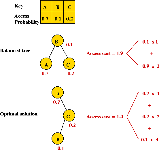
We are also given access frequencies (probabilities) , e.g.

Key	Access probability
A	0.4
B	0.1
C	0.2
D	0.1
E	0.2

(Thus, "A" is most frequently accessed).

Objective: design a data structure to enable accesses as rapidly as possible.

Past solutions we have seen:

Place keys in a balanced binary tree.
⇒ a frequently-accessed item could end up at a leaf.
Place keys in a linked list (in decreasing order of probability).
⇒ lists can be long, might required O(n) access time (even on average).
Use a self-adjusting data structure (list or self-adjusting tree).

In-Class Exercise 9.8: Consider the following two optimal-list algorithms:

Algorithm 1


Algorithm: optimalList (E, p)
Input: set of elements E, with probabilities p
      // Base case: single element list 
1.    if |E| = 1
2.        return list containing E
3.    endif
4.    m = argmax_i p(i)      // Which i gives the max
5.    front = new node with m
6.    list = optimalList (E - {m}, p - p_m)
7.    return list.addToFront (front)

Algorithm 2:


Algorithm: optimalList2 (E, p)
Input: set of elements E, with probabilities p
      // Base case: single element list 
1.    if |E| = 1
2.        return list containing E
3.    endif
4.    for i=0 to E.length
5.        front = new node with i
6.        list = optimalList2 (E - {i}, p)
7.        tempList = list.addToFront (front)
8.        cost = evaluate (tempList)
9.        if cost < bestCost
10.           best = i
11.           bestList = tempList
12.       endif
13.   endfor
14.   return bestList

Analyze the running time of each algorithm in terms of the number of list elements n.

Optimal binary search tree:

Analogue of the optimally-arranged list.
Idea: build a binary search tree (not necessarily balanced) given the access probabilities.
Example:
Overall objective: minimize average access cost:
- For each key i, let d(i) be its depth in the tree
  (Root has depth 1).
- Let p_i be the probability of access.
- Assume n keys.
- Then, average access cost = d(0)*p₀ + ... + d(n-1)*p_n-1.

In-Class Exercise 9.9: Which of the two list algorithms could work for the optimal binary tree problem? Write down pseudocode.

Dynamic programming solution:

First, sort the keys.
(This is easy and so, for the remainder, we'll assume keys are in sorted order).
Suppose keys are in sorted order:
- If we pick the k-th key to be the root.
  ⇒ keys to the left will lie in the left sub-tree and keys to the right will lie in the right sub-tree.
- This also works for any sub-range i, ..., j of the keys:
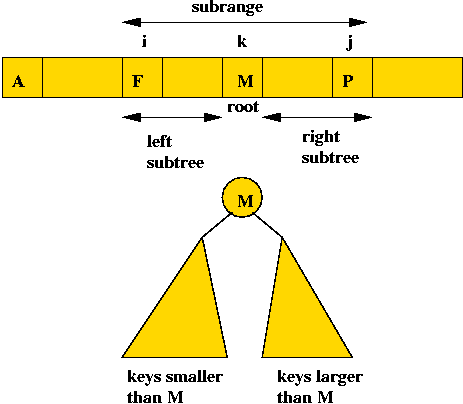
Define $C(i,j)$ = cost of an optimal tree formed using keys i, ..., j (both inclusive).
Now suppose, in the optimal tree, the root is "the key at position k".
- The left subtree has keys in the range i, ..., k-1.
  ⇒ optimal cost of left subtree is $C(i, k-1)$.
- The right subtree has keys k+1, ..., j.
  ⇒ optimal cost of right subtree is $C(k+1, j)$
It is tempting to assume that $C(i, j) = C(i, k-1) + C(k+1, j)$
⇒ this doesn't account for the additional depth of the left and right subtrees.
The correct relation is: $$ C(i,j) \eql p_k + C(i,k-1) + (p_i + \ldots + k_{k-1}) + C(k+1,j) + (p_{k+1} + \ldots + p_j) $$
To understand why this must be true, let's re-write $C(i, k-1)$ as $$ C(i,k-1) \eql (p_i d_i + \ldots + p_{k-1} d_{k-1}) $$ where the $d_i$'s are the depths of the items in $C(i, k-1)$.
Because $C(i, k-1)$'s depth increases by 1, in the larger tree, these items will have depth $d_i + 1$. Thus, the new depth is $$\eqb{ p_i (d_i + 1) + \ldots + p_{k-1} (d_{k-1} + 1) & = & (p_i + \ldots + p_{k-1}) + (p d_i + \ldots + p_{k-1} d_{k-1})\\ & = & (p_i + \ldots + p_{k-1}) + C(i,k-1)\\ }$$
The same argument applies to the right sub-tree and $C(k+1,j)$.
Therefore, $C(i, j)$ can be written more compactly as: $$ C(i,j) \eql C(i,k-1) + C(k+1,j) + (p_i + \ldots + p_j) $$
Now, we assumed the optimal root for $C(i, j)$ was the $k$-th key.
⇒ in practice, we must search for it.
⇒ consider all possible keys in the range i, ..., j as root.
Hence the dynamic programming recurrence is: $$ C(i,j) \eql \min_k \;\;\;\; C(i,k-1) + C(k+1,j) + (p_i + \ldots + p_j) $$ where $k$ ranges over $i, \ldots, j$.
The solution to the overall problem is: $C(0, n-1)$.
Observe:
- Once again, we have expressed the cost of the optimal solution in terms of the optimal cost of sub-problems.
- Base case: $C(i, i) = p_i$.

Implementation:

Writing code for this case is not as straightforward as in other examples:
- In other examples (e.g., load balancing), there was a natural sequence in which to "lay out the sub-problems".
- Consider the following pseudocode:
```
    // Initialize C and apply base cases. 
    for i=0 to numKeys-2
        for j=i+1 to numKeys-1
            min = infinity
            sum = p_i + ... + p_j;
            for k=i to j
                if C(i, k-1) + C(k+1, j) + sum < min
                    min = C(i, k-1) + C(k+1, j) + sum
          ...
    
```
  Suppose, above, i=0, j=10 and k=1 in the innermost loop
  - The case C(i, k-1) = C(0,0) is a base case.
  - But the case C(k+1, j) = C(2, 10) has NOT been computed yet.
- We need a way to organize the computation so that:
  - Sub-problems are computed when needed.
  - Sub-problems are not re-computed unnecessarily.

Solution using recursion:

Key idea: use recursion, but check whether computation has occurred before.

Pseudocode:


Algorithm: optimalBinarySearchTree (keys, probs)
Input: keys[i] = i-th key,  probs[i] = access probability for i=th key.

      // Initialize array C, assuming real costs are positive (or zero). 
      // We will exploit this entry to check whether a cost has been computed. 
1.    for each i,j set C[i][j] = -1;
      // Base cases: 
2.    for each i, C[i][i] = probs[i];

      // Search across various i, j ranges. 
3.    for i=0 to numKeys-2
4.        for j=i+1 to numKeys-1
              // Recursive method computeC actually implements the recurrence. 
5.            C[i][j] = computeC (i, j, probs)
6.        endfor
7.    endfor

      // At this point, the optimal solution is C(0, numKeys-1) 
8.    Build tree;
9.    return tree

Output: optimal binary search tree


Algorithm: computeC (i, j, probs)
Input: range limits i and j, access probabilities

     // Check whether sub-problem has been solved before. 
     // If so, return the optimal cost. This is an O(1) computation. 
1.   if (C[i][j] >= 0)
2.       return C[i][j]
3.   endif

     // The sum of access probabilities used in the recurrence relation. 
4.   sum = probs[i] + ... + probs[j];

     // Now search possible roots of the tree. 
5.   min = infinity
6.   for k=i to j
         // Optimal cost of the left subtree (for this value of k). 
7.       C_left = computeC (i, k-1)
         // Optimal cost of the right subtree. 
8.       C_right = computeC (k+1, j)
         // Record optimal solution. 
9.       if C_left + C_right < min
10.          min = C_left + C_right
11.      endif
12.  endfor

13.  return min

Output: the optimal cost of a binary tree for the sub-range keys[i], ..., keys[j].

Note: In the above pseudocode, we have left out a small detail: we need to handle the case when a subrange is invalid (e.g., when k-1 < i). Can you see how this case can be handled?

Analysis:

The bulk of the computation is a triple for-loop, each ranging over n items (worst-case)
⇒ O(n³) overall.
Note: we still have account for the recursive calls:
- Each recursive call that did not enter the innermost loop, takes time O(1).
- But, this occurs only O(n²) times.
  ⇒ Overall time is still O(n³).

Dynamic Programming: Summary

So, what to make of dynamic programming and its "strangeness"?

Key points to remember:

The method sets up a recurrence between sub-problems
⇒ solutions to sub-problems can be assembled into a solution to the actual problem of interest.
Sometimes, recursion is useful as the way to implement the recurrence. Sometimes not.
- Example: optimal binary tree (recursion works).
- Example: Floyd-Warshall (recursion does not work).
The recurrence is set up in terms of the optimal "cost" or "value" of a sub-problem solution.
- Example: In Floyd-Warshall, the cost D^k_ij is the cost of a shortest-path.
- Example: In optimal trees, C(i,j) is the optimal access time.
If the recurrence can be set up, a problem is a potential candidate for dynamic programming.
Just because dynamic programming can be set up doesn't mean it will be the most efficient solution.

In-Class Exercise 9.10: For the moment, let's set aside efficiency and merely get some practice with seeing if dynamic programming can be set up properly. Consider an array A with n elements and the following three problems:

Let $D_{ij} = \max_{i\leq m\leq j} A[m]$, the largest value in the range $i$ to $j$.

Let $D_{ij} = \max_{i\leq m,n\leq j} A[m]+A[n]$, the largest sum of two elements in the range $i$ to $j$.

Let $D_{ij} = \max_{i\leq m < j} A[m]+A[m+1]$, the largest sum of two consecutive elements in the range $i$ to $j$.

For each of the above problems, can $D_{ij}$ be written in terms of $D_{ik}$ and $D_{kj}$ where $i\leq k\leq j$, with possibly a few additional terms like $A[k]$?