Week 12: Modules and Classes

Reading: Python for Data Analysis Chapter 4, through “Boolean Indexing”

Notes

The NumPy Array

Python did not originally have dedicated features for numerical computing: these were added later in a library called NumPy (or numpy).

Check to see if you have NumPy installed by importing it:

import numpy as np

The convention import numpy as np exists entirely to save us some typing. It is widespread: almost every reference on numpy will use it, so we will use it here.

The basic data type in numpy is the array. It’s similar to a list, but better for doing math. It’s also, formally, an object of the class numpy.ndarray.

Note: ndarray means “n-dimensional array” - we will just call it an array.

Recall that the + operator between lists concatenates lists:

x = [2, 3, 4]

y = [1, 2, 3]

x + y

[2, 3, 4, 1, 2, 3]

We create numpy arrays by using the np.array function called on a list:

x_arr = np.array(x)

type(x)

list

type(x_arr)

numpy.ndarray

Construction

Every class has a function that creates a new instance of the class (a new object). That function has the same name as the class, and is formally called the constructor.

Arrays are very useful for mathematical operations. Note how the + operator adds the two arrays, element by element:

y_arr = np.array(y)

x_arr

array([2, 3, 4])

y_arr

array([1, 2, 3])

x_arr + y_arr

array([3, 5, 7])

Arrays also support other mathematical operations:

x_arr - y_arr

array([1, 1, 1])

x_arr * y_arr

array([ 2,  6, 12])

x_arr / y_arr

array([2.        , 1.5       , 1.33333333])

Arrays can be used for math with regular numbers (scalars):

x_arr + 2

array([4, 5, 6])

The number is broadcast across the entire array.

Linear Algebra

If you’ve had a linear algebra class, you might want to use numpy arrays for tensor operations.

The @ operator performs matrix multiplication
The .T value of an array is its transpose

np.array([[1, 2],[3, 4]]) @ np.array([[1, 2]]).T

array([[ 5],
       [11]])

Numpy arrays can also be indexed similarly to lists:

x_arr[1]

np.int64(3)

x_arr[1] += 1

x_arr[1]

np.int64(4)

Numpy arrays have some substantial differences from lists. For instance, you cannot use .append with a numpy array.

Properties of Objects

Numpy arrays are objects, which collect variables and functions together logically. When functions are associated with objects, we refer to them as methods.

We can contrast these objects with “primitive” types like ints and floats.

You’ve seen some object-like properties already with strings:

x = "George"
y = x.lower()
print(y)

george

The string class has a method lower() associated with it - you call lower() on a string with a period between the name of the variable and the name of the method.

Numpy arrays have a great number of useful methods.

Consider the task of finding the index of a list corresponding to the largest value. The list [3, 7, 4, 2] has the largest value at index 1 (the second item). Numpy arrays have a method, argmax (argument maximum) for this:

x = np.array([3, 7, 4, 2])
y = x.argmax()
print(y)

Another method, reshape changes the shape of an array:

x = np.array([1, 2, 3, 4])
z = x.reshape(2, 2)
print(z)

[[1 2]
 [3 4]]

…but what is the “shape” of an array? Objects in Python have variables associated with them. We can access these like other variables, associating them with the object using a decimal.

x = np.array([[1, 2, 3]])
print("x:\n", x)
print("x.shape:\n", x.shape)
y = x.reshape(3, 1)
print("y:\n", y)
print("y.shape:\n", y.shape)

x:
 [[1 2 3]]
x.shape:
 (1, 3)
y:
 [[1]
 [2]
 [3]]
y.shape:
 (3, 1)

Numpy arrays also have a size: the total number of numbers in the array:

x = np.array([[10, 11, 20, 21]])
print("x:\n", x)
print("x.size:\n", x.size)
y = x.reshape(2, 2)
print("y:\n", y)
print("y.size:\n", y.size)

x:
 [[10 11 20 21]]
x.size:
 4
y:
 [[10 11]
 [20 21]]
y.size:
 4

There’s a relationship between size and shape: the size is the product of the dimensions of the shape multiplied together. Some shapes are invalid: for instance, an array of size 7 can’t be reshaped to (4, 2): there’s no logical way to put 7 things into eight places.

Extra! Randomness, Simulation, and Plots

This material is optional.

Many early and contemporary uses of computing involve simulation: calculating a value approximately by simulating events. Events can be simulated through randomness.

We can generate a random number with numpy:

np.random.random()

0.6824172279670319

np.random.random() gives us a random number in between 0 and 1.

Let’s use this to create a “coin”:

coin.py

import numpy as np

def flip():
    rand_number = np.random.random()
    if rand_number > 0.5:
        return "Heads"
    else:
        return "Tails"

print(flip())

Tails

Let’s test our “coin” (include all of this in one file):

trials = 10000
results = 0
for j in range(trials):
    if flip() == "Heads":
        results += 1
print(results/trials)

0.5004

About 50% - it works!

We can also randomly choose an element from a list:

np.random.choice(["bricks", "lumber", "cement"])

np.str_('lumber')

Let’s use randomness to simulate a simple problem: estimating the value of \(\pi\).

Assume:

We know that the formula for a circle is given by \(x^2 + y^2 = r^2\)
We know the area of a square is \(s^2\)
We know the area of a circle is \(\pi \cdot r^2\)
We don’t know the value of \(\pi\)

First, let’s use our random number generator to get values in between -1 and 1.

By default, np.random.random() gives values between 0 and 1. To get values between -1 and 1:

Double the default random values
- This places them between 0 and 2 instead of 0 and 1
Subtract one from the doubled value
- This places them between -1 and 1

( np.random.random() * 2 ) - 1

0.5169177108281502

Now let’s write a function that generates one point and returns it:

def generate_point():
    x = np.random.random() * 2 - 1
    y = np.random.random() * 2 - 1
    return x, y

generate_point()

(0.7749061521554383, 0.37564972347930525)

We can use another function to check if a point is inside the circle:

def check_point(x, y):
    if x**2 + y**2 <= 1:
        return True
    else:
        return False

check_point(0, 0)

True

check_point(1, 1)

False

Now let’s generate a lot of points, check all of them, and count the ones inside the circle:

num_points = 1000000
in_circle = 0
for j in range(num_points):
    x, y = generate_point()
    result = check_point(x, y)
    if result:
        in_circle += 1
print(in_circle)

Finally, let’s check the ratio of points in the circle to total points. We’ll multiply it by four, because the side of the “square” we are using is 2, and we’re looking at the ratio: \[\frac{\pi \cdot r^2}{(2\cdot r)^2} = \frac{\pi \cdot r^2}{4 \cdot r^2} \]

ratio = in_circle/num_points
print(ratio * 4)

3.141952

The answer is reasonably close to \(\pi\), and if we make the number of points larger, the result will become more accurate.

Plotting

We will use Python to plot charts of our results, using a library called seaborn.

Plotting is a good way to communicate numerical information visually. We’ll show you a few things about plotting, but this course won’t require you to make plots or test you on plotting.

To follow along, you can install seaborn by typing pip install seaborn at your terminal.

Plotting with Python is much more powerful and expressive than plotting with a spreadsheet program such as Microsoft Excel. We will present an ‘extra’ lesson on plotting at the end of the course.

Let’s plot the results. First, we need to import a plotting library:

import seaborn as sns
import matplotlib.pyplot as plt

Next, we need to remember the x and y values we generated, so we modify our loop to do so:

num_points = 1000000
x_circ, y_circ = [], [] # lists for values in circle
x_no_circ, y_no_circ = [], [] # lists for values out of circle
for j in range(num_points):
    x, y = generate_point()
    result = check_point(x, y)
    if result:
        x_circ.append(x)
        y_circ.append(y)
    else:
        x_no_circ.append(x)
        y_no_circ.append(y)

We can check the result: this time, we’ll look at the length of one of the lists of “in circle” values:

ratio = len(x_circ)/num_points
print(ratio * 4)

3.141876

Now we’ll plot the result:

sns.set_theme(rc={'figure.figsize':(6,6)})
sns.scatterplot(x=x_circ, y=y_circ)
sns.scatterplot(x=x_no_circ, y=y_no_circ)
plt.show()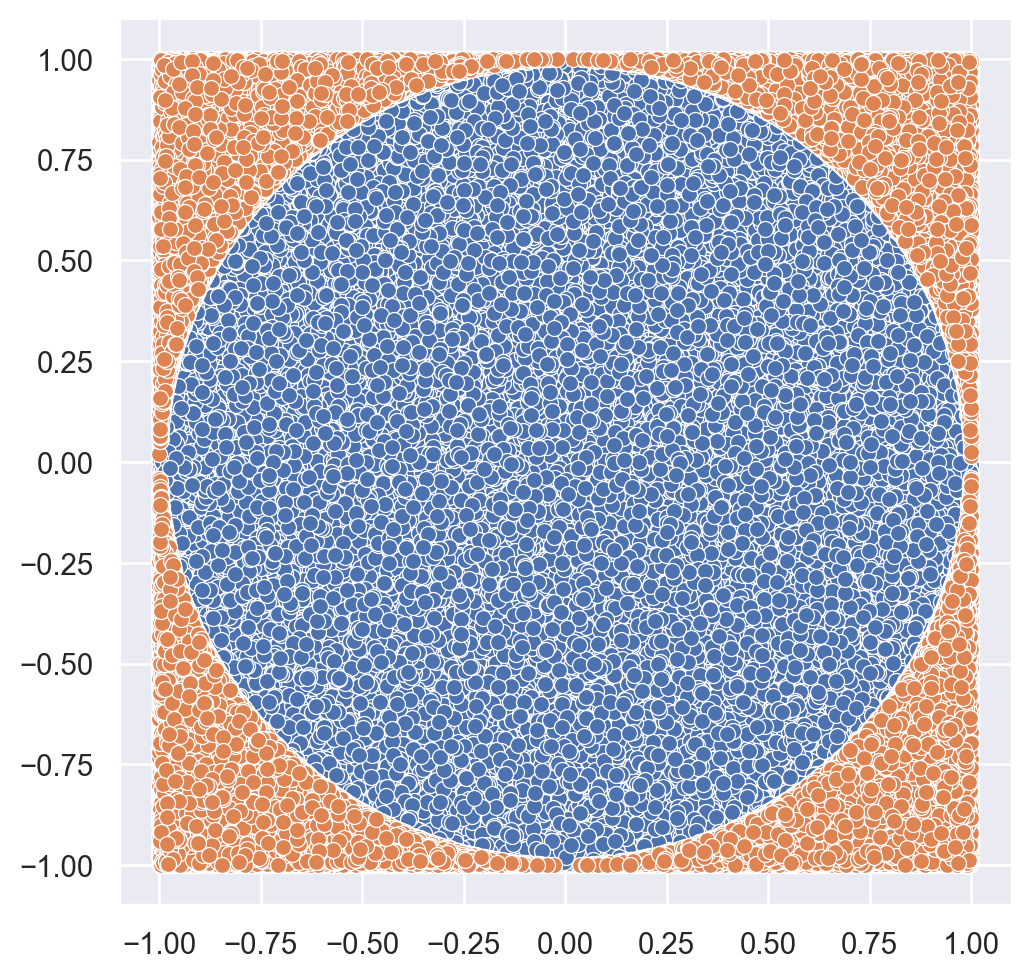

Practice Problem (Optional)

Estimate the value of \(\pi\) with a circle of radius 2 (our example had radius 1).

Practice

Practice Problem 12.1

Write a function to_numpy that takes as argument a list and returns:

A numpy array of the same values, if every element of the list is numeric
The bool False if any element of the list is non-numeric.

Practice Problem 12.2

Write a function compare_lists that takes two lists of ints and compares each pair of elements, returning a list of bools corresponding to whether the first list’s element is greater:

compare_lists([2, 3, 4], [3, 1, 2]) returns [False, True, True]
- 2 is not greater than 3, 3 is greater than 1, 4 is greater than 2

Practice Problem 12.3

Write a function list_ceil that takes two arguments:

The first argument a list of ints
The second argument is a single int

The function should return a new list, identical to the original list, except no int in the new list is greater than the second argument.

list_ceil([3, 5, 2, 1], 4) returns [3, 4, 2, 1]
list_ceil([-1, 0, 6, 1], 2) returns [-1, 0, 2, 1]

Practice Problem 12.4

Write a function array_mean that takes as argument a numpy array, calculates the mean, subtracts it from the array, and returns it.

Practice Problem 12.4

Write a function reshaper that takes two arguments:

The first argument is a numpy array
The second argument is a tuple representing a shape

If the array can be reshaped into the new shape, return an array in the new shape. If the array can’t be reshaped, return boolean False.

Homework

Homework problems should always be your individual work. Please review the collaboration policy and ask the course staff if you have questions. Remember: Put comments at the start of each problem to tell us how you worked on it.
Double check your file names and return values. These need to be exact matches for you to get credit.
This homework includes 20 pts bonus - you can earn extra credit on this assignment.

Homework Problem 12.1

Homework Problem 12.1 (25 pts)

Write a function percentage_diff that takes as argument two lists of numbers:

If the second list does not contain any zeroes, calculate the percentage difference between corresponding elements in the lists, and return the result as a numpy array. You should calculate the percentage difference between an element, A, in the first list and an element, B, in the second list as follows: \(\frac{(A-B)*100}{B}\)
If the second list contains zeroes, return False

Examples:

percentage_diff([2, 3, 2], [1, 3, 4]) returns numpy array [100., 0., -50.]
- \(\frac{(2-1)*100}{1} = 100\)
- \(\frac{(3-3)*100}{3} = 0\)
- \(\frac{(2-4)*100}{4} = -50\)
percentage_diff([4, 5, 1], [3, 0, 2]) returns False
- The second list contains a zero

Submit as percentage_diff.py.

Homework Problem 12.2

Homework Problem 12.2 (25 pts)

Write a function valid_shapes that takes one argument, a numpy array. The array will be two-dimensional.

Your function should return a list of tuples of valid shapes (in two dimensions) that the array could be reshaped into. The list can be in any order, provided it has the correct contents.

valid_shapes(np.array([[3, 4, 5, 6]])) returns [(4, 1), (2, 2), (1, 4)]
valid_shapes(np.array([[3, 4, 5, 6, 7]])) returns [(5, 1), (1, 5)]
valid_shapes(np.array([[1, 3, 4], [1, 5, 6]])) returns [(6, 1), (3, 2), (2, 3), (1, 6)]

Submit as valid_shapes.py.

Hints and Notes

What is the size of the input array?
What numbers can be multiplied together to yield the size?
- Recall the greatest_factor problem from earlier in the course.
- You will want to check a series of possible values with a loop.
- Those values will always be greater than or equal to one 1, and less than or equal to the array size.

Note: There are “one dimensional” numpy arrays that have shapes like (4,) — this is different from (4, 1). Don’t worry about these!

Homework Problem 12.3

Homework Problem 12.3 (50 pts)

A list of integers might have some integers in sequential order:

[2, 3, 4, 1, 5, 6, 8] has 2, 3, and 4 in order and 5 and 6 in sequential order
[4, 7, 8, 9, 2] has 7, 8, and 9 in order

An alternate representation of such a list would be to capture the sequences with the first and last element of each sequence by using a list within a list:

[2, 3, 4, 1, 5, 6, 8] could be represented as [[2, 4], 1, [5, 6], 8]
[4, 7, 8, 9, 2]could be represented as [4, [7, 9], 2]
[1, 3, 4, 5, 6, 7, 8, 9, 10]could be represented as [1, [3, 10]]

Write a function compressor that takes a list of integers and returns a list in this alternate representation.

Submit as compressor.py.

Homework Problem 12.4

Homework Problem 12.4 (20 pts)

Write a function that reverses the compressor function from the previous problem: take the alternate representation and return the original list representation.

Submit as compressor_reverser.py.