import numpy as np
import pandas as pd
import seaborn as snsModule 2.1 - Data
Objectives
This module introduces the pandas data analysis library. The name “pandas” is a reference to Python Data Analysis (it is not a perfect acronym), that also references a mammal.
Optional Multimedia Content (Photograph of Red Panda)

(Image: Public Domain)
We also introduce the seaborn library, used for plotting. You have used drawtool for some plotting tasks already: drawtool is a simplified library that performs simple plotting functions. Learning the basics of pandas and seaborn will prepare you for more advanced plotting and data analysis in the future.
2.1.0 - Setup
Try running this simple program:
If it runs without error, everything is working. If not, review the installation instructions from the beginning of the course - particularly for Thonny users, the Library Installation step is necessary.
Note also the convention to import pandas as pd, similar to how we imported numpy as np. This is only a convention, but it is an extremely common one.
2.1.1 - The Series
You’re already familiar with basic Python lists and Numpy arrays. Pandas has a similar data structure called a Series. Let’s look at a simple example.
import pandas as pd

x = pd.Series([1, 2, 4, 7])
print(x)
0 1
1 2
2 4
3 7
dtype: int64Series is capitalized!
Just like everything else in Python, capitalization of code is important here.
import pandas as pd

a = pd.series([1, 2, 4, 7])
print(a)
Note the index of the pandas Series: each element of the Series explicitly has an index, here values 0 through 3, associated with it.
The indices here are similar to the indices of a list of a Numpy array. “Zero-indexing” in this fashion is the default for a pandas Series.
More Information Than You Require
The dtype (data type) of the Series values, int64 is also shown. int64 stands for “64-bit integer”, where 64-bit specifies the maximum size the integer can take on. The dtype can be useful for doing some advanced computation, but you can safely ignore it for this module.
Numerical indices for a pandas Series can be overridden by explicitly providing an index argument when the Series is created:
import pandas as pd

hurricane_years = pd.Series([2005, 2012, 2011, 2022],
                       index=["Katrina", "Sandy", "Irene", "Ian"])
print(hurricane_years)
Katrina 2005
Sandy 2012
Irene 2011
Ian 2022
dtype: int64- In addition to the Series values of
[2005, 2012, 2011, 2022], we used the argumentindex=["Katrina","Sandy","Irene","Ian"]to specify the indices for the values. - Using
index=here is similar to usingend=in aprintstatement: it is an argument that overrides a default behavior. - We passed in a list of strings for
index, and the values of the list became the indices for the elements of the Series in corresponding order. - There is a line break after the comma. This is a stylistic choice in writing code:
- In general, anywhere in Python code where there is a comma (such as lists, dictionaries, Numpy arrays, function arguments, etc.), you may insert a line break, and Python will start to “read” the code on the next line, ignoring all spacing.
- This is optional, and meant to help “organize” code visually as you write it.
- It is common when working with data, to prevent lines from getting long and hard to read.
- It never applies inside of a string.
Exercise 2.1.1
Series elements can be accessed by index name, similar to how list elements are accessed by index.
When indices are the default numbers, the behavior is identical:
import pandas as pd

x = pd.Series([1, 2, 4, 7])
print(x[3])7When indices are named, the behavior resembles that of a dictionary:
import pandas as pd

hurricane_years = pd.Series([2005, 2012, 2011, 2022],
                       index=["Katrina", "Sandy", "Irene", "Ian"])
print(hurricane_years["Irene"])2011We can also pass in a list of indices in this manner! This returns a new Series consisting of the elements we selected. Similar to accessing a single element, it does not modify the original Series.
import pandas as pd

x = pd.Series([1, 2, 4, 7])

hurricane_years = pd.Series([2005, 2012, 2011, 2022],
                       index=["Katrina", "Sandy", "Irene", "Ian"])
print(x[[2,3]])
print()
print(hurricane_years[["Irene", "Katrina"]])
2 4
3 7
dtype: int64
Irene 2011
Katrina 2005
dtype: int64- Note that the single value inside of square brackets is replaced by a list inside of square brackets: the square brackets are nested.
- The new Series from
hurricane_yearsis in a different order. When accessing by indices in this manner, you can select whichever elements you like in whatever order you like.
We can also do more sophisticated selection using conditionals. Here we are selecting data from the hurricane_years Series based on the value of hurricane_years being greater than or equal to 2012: selecting storms from 2012 or later.
import pandas as pd

hurricane_years = pd.Series([2005, 2012, 2011, 2022],
                       index=["Katrina", "Sandy", "Irene", "Ian"])

print(hurricane_years[hurricane_years >= 2012])
Sandy 2012
Ian 2022
dtype: int64We’ve seen how to create a Series with two lists (one of data, one indices). We’ve also seen some dictionary-like behavior of Series. It is also possible to create a Series from a dictionary:
import pandas as pd

hurricane_wind_speed = pd.Series({'Katrina': 280, 'Sandy': 185, 'Irene': 195, "Ian": 250})

print(hurricane_wind_speed)
Katrina 280
Sandy 185
Irene 195
Ian 250
dtype: int64These hurricane wind speeds are in kilometers per hour. What if we want to convert to miles per hour?
You can perform mathematical operations on a pandas Series, similar to NumPy array. The conversion rate between kph and mph is about 0.621:
import pandas as pd

hurricane_wind_speed = pd.Series({'Katrina': 280, 'Sandy': 185, 'Irene': 195, "Ian": 250})

print(hurricane_wind_speed*0.621)
Katrina 173.880
Sandy 114.885
Irene 121.095
Ian 155.250
dtype: float64You can also perform basic math operations between two pandas Series, and the operations will be performed according to each index:
import pandas as pd

# damage in millions of US dollars as of year of hurricane
hurricane_damage_estimate = pd.Series({'Katrina': 122800, 'Sandy': 67300,
                                       'Irene': 15500, 'Ian': 112100})
hurricane_damage_update = pd.Series({'Ian': 1000, 'Katrina': 2200,
                                     'Irene': -1300, 'Sandy': 1400})
hurricane_damage_final = hurricane_damage_estimate + hurricane_damage_update

print(hurricane_damage_final)
Ian 113100
Irene 14200
Katrina 125000
Sandy 68700
dtype: int64The above calculation simulates updating an original estimate by a small amount.
Exercise 2.1.2
In summary: the pandas Series is a very flexible type of data structure, combining elements of dictionaries, lists, and NumPy arrays, useful for data analysis.
2.1.2 - The DataFrame
While the Pandas Series is useful on its own, it is also a building block for an even more useful data structure: the Pandas DataFrame.
- A DataFrame is a two-dimensional data structure, somewhat similar to a spreadsheet.
- A DataFrame can represent more dimensions, but we will use it in two dimensions
- A DataFrame can represent more dimensions, but we will use it in two dimensions
- A DataFraem consists of rows and columns.
- Formally, a DataFrame is a collection of columns, each of which is a named Pandas Series.
DataFrames can be created in many ways. One way is to use a dictionary of lists:
import pandas as pd

hurricanes = {'name': ["Katrina", "Sandy", "Irene", "Ian"],
              'year':[2005, 2012, 2011, 2022],
              'wind speed': [280, 185, 195, 250],
              'damage': [122800, 67300, 15500,  112100]}

hurricane_df = pd.DataFrame(hurricanes)
print(hurricane_df)
name year wind speed damage
0 Katrina 2005 280 122800
1 Sandy 2012 185 67300
2 Irene 2011 195 15500
3 Ian 2022 250 112100Note how the
pd.DataFrame()function was called on the dictionary of named lists to create the DataFrame.Printing a DataFrame displays a text table of the contents.
The DataFrame can be “indexed” directly by column.
Code Blocks
The code below continues the code above - all of the code in Section 2.1.2 will form one long program.
print(hurricane_df['name'])0 Katrina
1 Sandy
2 Irene
3 Ian
Name: name, dtype: objectThis output looks just like a Pandas Series because it is a Pandas Series!
print(type(hurricane_df['name']))<class 'pandas.core.series.Series'>What if want to add in another Series to the DataFrame? Let’s try including the damage update values:
hurricane_damage_update = pd.Series({'Ian': 1000, 'Katrina': 2200,
                                     'Irene': -1300, 'Sandy': 1400})
hurricane_df['damage update'] = hurricane_damage_update

print(hurricane_df)
name year wind speed damage damage update
0 Katrina 2005 280 122800 NaN
1 Sandy 2012 185 67300 NaN
2 Irene 2011 195 15500 NaN
3 Ian 2022 250 112100 NaNThis did not work!
NaN means “not a number” - the new Series was not added to the DataFrame correctly. Importantly, there was no error: the code runs, but we don’t get the output we want.
To get this to work, the index values for the DataFrame must be the same as the index values for the Series. Right now, the DataFrame indices are numerical, 0 through 3. We can change this to any column’s values using the DataFrame.set_index function:
hurricane_df = hurricane_df.set_index('name')
print(hurricane_df)
year wind speed damage damage update
name
Katrina 2005 280 122800 NaN
Sandy 2012 185 67300 NaN
Irene 2011 195 15500 NaN
Ian 2022 250 112100 NaNThe index values are now the values of the column 'name'!
Note, importantly, that even though the set_index function belongs to the DataFrame (hence hurricane_df.set_index), we must assign the result: hurricane_df = hurricane_df.set_index('name'). This function does not modify the DataFrame in place.
Now we can add a new Series to the DataFrame:
hurricane_df['damage update'] = hurricane_damage_update

print(hurricane_df)
year wind speed damage damage update
name
Katrina 2005 280 122800 2200
Sandy 2012 185 67300 1400
Irene 2011 195 15500 -1300
Ian 2022 250 112100 1000Let’s take a closer look at the syntax:
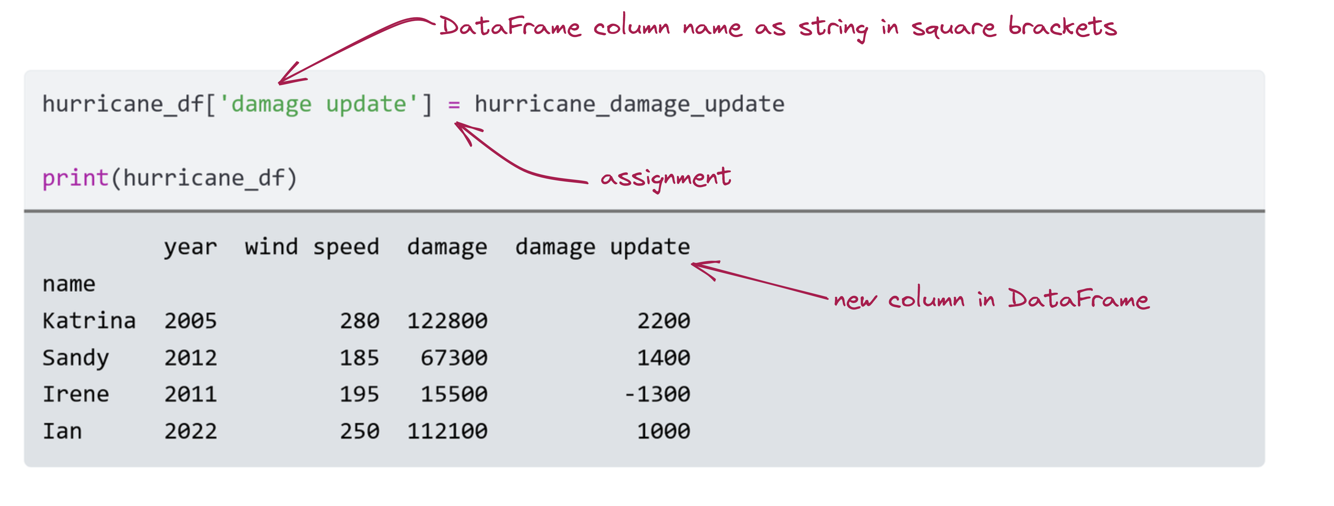
- Creating/modifying a column in a DataFrame is similar to creating a new element in a dictionary
- The column name is in square brackets
- Here it is a string (but you could use an int or a float)
- The assignment operator
=is used to assign some new value or values to the column.- If you use a single value, it will be assigned to every entry in the column
- If you use a list or NumPy array, the values will be assigned in sequential order
- If you use a Pandas Series, the indices must match (and values will be assigned according to indices)
We saw previously that math operators worked on Pandas Series, and since Pandas Series are the building blocks of Pandas DataFrames, we can use that functionality within DataFrames too:
hurricane_df['damage final'] = hurricane_df['damage'] + hurricane_df['damage update']

hurricane_df['wind speed (mph)'] = hurricane_df['wind speed'] * 0.621

print(hurricane_df)
year wind speed damage damage update damage final \
name
Katrina 2005 280 122800 2200 125000
Sandy 2012 185 67300 1400 68700
Irene 2011 195 15500 -1300 14200
Ian 2022 250 112100 1000 113100
wind speed (mph)
name
Katrina 173.880
Sandy 114.885
Irene 121.095
Ian 155.250 Now that we have two different wind speeds, we might want to rename the old column to reflect that the speed is measured in kilometers per hour. We do this with the DataFrame.rename function:
# pass columns to rename as a dictionary
# the keys are the old names, the values are the new names
columns_to_rename={'wind speed': 'wind speed (kph)'}

hurricane_df = hurricane_df.rename(columns=columns_to_rename)

print(hurricane_df)
year wind speed (kph) damage damage update damage final \
name
Katrina 2005 280 122800 2200 125000
Sandy 2012 185 67300 1400 68700
Irene 2011 195 15500 -1300 14200
Ian 2022 250 112100 1000 113100
wind speed (mph)
name
Katrina 173.880
Sandy 114.885
Irene 121.095
Ian 155.250 The syntax is important:
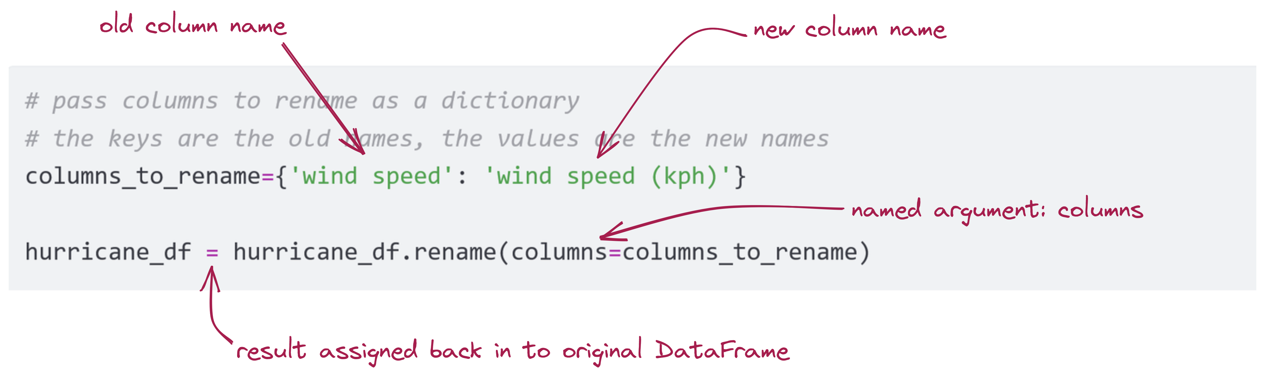
- The
DataFrame.renamefunction takes a named argument,column, telling us that we’re renaming one or more columns - We created a variable to use as that argument: a dictionary
- The dictionary keys are the ‘old’ column names
- The corresponding values are what we are renaming the columns to
- The result of calling this function is a new DataFrame.
- Here, we assign this back into the old variable name
- If we did not perform this assignment,
hurricane_dfwould not have changed.
If we want to remove a column, we can use the DataFrame.drop function. The syntax is similar.
# pass columns to remove as a list
# list items are the names of columns to remove
columns_to_drop=['damage', 'damage update', 'wind speed (kph)']

hurricane_df = hurricane_df.drop(columns=columns_to_drop)

print(hurricane_df)
year damage final wind speed (mph)
name
Katrina 2005 125000 173.880
Sandy 2012 68700 114.885
Irene 2011 14200 121.095
Ian 2022 113100 155.250If you use a different named argument from columns, the DataFrame.rename and DataFrame.drop functions will do different things. Specifically useful is the named argument index, which refers to rows in the DataFrame by index name.
hurricane_df.drop(index=['Sandy'])The code above drops the row with index 'Sandy' from the DataFrame.
Be careful! Just like dropping a column, this function returns a new DataFrame: the result must be assigned if you want to use it.
Exercise 2.1.3
2.1.3 - Data I/O
While being able to manage data in the spreadsheet-like format of a DataFrame is an advantage over maintaining a bunch of Series individually, in the example above we still populated the DataFrame manually.
Wouldn’t it be nice if we could read data from a file into a DataFrame directly?
Pandas offers just such functionality via methods to read and write from csv files.
A csv file, which has a .csv extension, stands for Comma Separated Variable, and refers to a file where each row is like a row in a spreadsheet, while each column is separated from other columns with a comma.
Here is an example of what such a file would look like if you opened it in your text editor:
BEGIN_YEARMONTH,BEGIN_DAY,BEGIN_TIME,END_YEARMONTH,END_DAY,END_TIME,EPISODE_ID,EVENT_ID,STATE,STATE_FIPS,YEAR,MONTH_NAME,EVENT_TYPE,CZ_TYPE,CZ_FIPS,CZ_NAME,WFO,BEGIN_DATE_TIME,CZ_TIMEZONE,END_DATE_TIME,INJURIES_DIRECT,INJURIES_INDIRECT,DEATHS_DIRECT,DEATHS_INDIRECT,DAMAGE_PROPERTY,DAMAGE_CROPS,SOURCE,MAGNITUDE,MAGNITUDE_TYPE,FLOOD_CAUSE,CATEGORY,TOR_F_SCALE,TOR_LENGTH,TOR_WIDTH,TOR_OTHER_WFO,TOR_OTHER_CZ_STATE,TOR_OTHER_CZ_FIPS,TOR_OTHER_CZ_NAME,BEGIN_RANGE,BEGIN_AZIMUTH,BEGIN_LOCATION,END_RANGE,END_AZIMUTH,END_LOCATION,BEGIN_LAT,BEGIN_LON,END_LAT,END_LON,EPISODE_NARRATIVE,EVENT_NARRATIVE,DATA_SOURCE
195004,28,1445,195004,28,1445,,10096222,"OKLAHOMA",40,1950,"April","Tornado","C",149,"WASHITA",,"28-APR-50 14:45:00","CST","28-APR-50 14:45:00","0","0","0","0","250K","0",,"0",,,,"F3","3.4","400",,,,,"0",,,"0",,,"35.12","-99.20","35.17","-99.20",,,"PUB"
195004,29,1530,195004,29,1530,,10120412,"TEXAS",48,1950,"April","Tornado","C",93,"COMANCHE",,"29-APR-50 15:30:00","CST","29-APR-50 15:30:00","0","0","0","0","25K","0",,"0",,,,"F1","11.5","200",,,,,"0",,,"0",,,"31.90","-98.60","31.73","-98.60",,,"PUB"
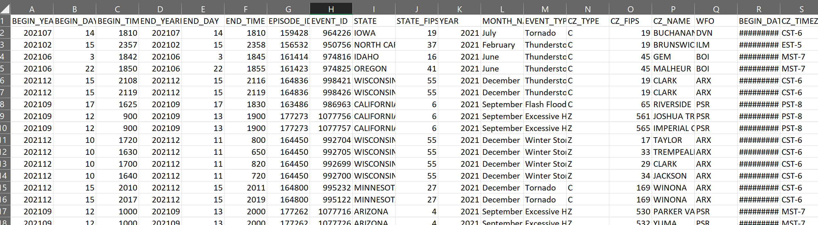
195007,5,1800,195007,5,1800,,10104927,"PENNSYLVANIA",42,1950,"July","Tornado","C",77,"LEHIGH",,"05-JUL-50 18:00:00","CST","05-JUL-50 18:00:00","2","0","0","0","25K","0",,"0",,,,"F2","12.9","33",,,,,"0",,,"0",,,"40.58","-75.70","40.65","-75.47",,,"PUB"Above, we see the first few rows of a csv file that is storing information about storm events, downloaded from NOAA. If we opened the same csv file in MS Excel, the first few rows and columns look like this:
Download a copy of the file, storm_events_details.csv to your computer. You can get the data directly from NOAA through the above link, but we have done a small amount of pre-processing to make it easier to work with for our class.
Try opening the file, once you’ve downloaded it, in MS Excel or Google Sheets; we will be using it in the next few exercises.
Once you have a csv file on your computer, you need to know its path on your machine so that you can send this information to pandas to open the file for you.
- The easiest way to do this is to copy the csv into the same folder/directory where you have the
.pyfile you’re running.- Then, you can simply use the file name,
storm_events_details.csv
- Then, you can simply use the file name,
- Otherwise, you’ll have to provide the absolute path of the file, which is something like
C:\Users\yourusername\Downloads\storm_events_details.csvto the function.
Let’s assume both our python file and the csv above are in the same folder. Then, using pandas, we can load the csv into a DataFrame directly with the following code:
storm_data = pd.read_csv('storm_events_details.csv')
print(storm_data.head())
BEGIN_YEARMONTH BEGIN_DAY BEGIN_TIME END_YEARMONTH END_DAY END_TIME \
0 202107 14 1810 202107 14 1810
1 202102 15 2357 202102 15 2358
2 202106 3 1842 202106 3 1845
3 202106 22 1850 202106 22 1855
4 202112 15 2108 202112 15 2116
EPISODE_ID EVENT_ID STATE STATE_FIPS ... END_RANGE \
0 159428 964226 IOWA 19 ... 3.0
1 156532 950756 NORTH CAROLINA 37 ... 4.0
2 161414 974816 IDAHO 16 ... 2.0
3 161423 974825 OREGON 41 ... 0.0
4 164836 998421 WISCONSIN 55 ... 0.0
END_AZIMUTH END_LOCATION BEGIN_LAT BEGIN_LON END_LAT END_LON \
0 S AURORA 42.580 -91.7200 42.5800 -91.7200
1 S CAMP BRANCH 34.127 -78.3541 34.1278 -78.3508
2 ESE LETHA 43.890 -116.6400 43.8895 -116.6058
3 NW ONTARIO 44.020 -117.0200 44.0310 -116.9711
4 W GLOBE 44.540 -90.7600 44.6500 -90.6800
EPISODE_NARRATIVE \
0 Severe thunderstorms developed ahead of an app...
1 Strong low pressure and a cold front produced ...
2 Sufficient daytime heating lead to isolated af...
3 Hot and dry conditions were ideal for thunders...
4 An intense storm system moved across the Upper...
EVENT_NARRATIVE DATA_SOURCE
0 Brief touchdown in a field with no visible dam... CSV
1 A few hundred trees were snapped or uprooted b... CSV
2 Branches knocked down with photo. Personal Wea... CSV
3 The ASOS at Ontario reported a 62 MPH thunders... CSV
4 A path of wind damage occurred across southwes... CSV
[5 rows x 51 columns]If you run this code, you will see the DataFrame printed to the terminal. The read_csv function automatically knows to look for commas as separators in the file. The formal word for such a separator is a delimiter.
We use the DataFrame.head() function here to only print the beginning of the DataFrame for a very large amount of data, the terminal is not a useful place to inspect the entire data set.
Other Separator Characters
You also have the option of specifying this delimiter manually, for example, if you used the # instead of commas for separating columns in your csv:
df = pd.read_csv('data.csv', delimiter='#')Any arbitrary character can be used.
Sometimes, the data you’re loading might already have the columns specified as the first row in the file; our storm data looks like this. In such cases, pandas tries to manually infer that the column information exists.
You can turn this setting off by telling the function not to treat the first line as a header explicitly:
storm_data = pd.read_csv('storm_events_details.csv', header=None)
print(storm_data.head())
This will probably give you a warning, because the first row is now interpreted as data in each column and is of a different type than some of the data.
We can not only open a file and load it into a DataFrame, but also do the reverse: save a DataFrame to a file. With pandas, the function to do this is below:
storm_data.to_csv('my_storm_data.csv')The code above will save the entire DataFrame, including the header column names, to a file called my_storm_data.csv in the same directory as the .py file you are using.
2.1.4 - Applying Functions to Data
Now that we have access to very large datasets, we can start to perform analysis. First, let’s take a look at the contents of our DataFrame by calling a function that counts how many times a unique value appears in a column. For example, we could see which states had the most storm events in our dataset with:
print(storm_data['STATE'].value_counts())STATE
TEXAS 4623
CALIFORNIA 2820
NEW YORK 2395
VIRGINIA 2301
PENNSYLVANIA 2250
...
LAKE ONTARIO 12
VIRGIN ISLANDS 7
ST LAWRENCE R 4
HAWAII WATERS 2
E PACIFIC 2
Name: count, Length: 67, dtype: int64The default output sometimes gets compressed with a ... entry at the terminal. To see everything, use a loop:
Note that the result of value_counts() is a Pandas series:
print(type(storm_data['STATE'].value_counts()))<class 'pandas.core.series.Series'>We can use the Series’ item() function to get each item:
Looping With the
item() Function
for item in storm_data['STATE'].value_counts().items():
  print(item)
('TEXAS', 4623)
('CALIFORNIA', 2820)
('NEW YORK', 2395)
('VIRGINIA', 2301)
('PENNSYLVANIA', 2250)
('KANSAS', 1962)
('SOUTH DAKOTA', 1860)
('COLORADO', 1844)
('IOWA', 1786)
('MISSOURI', 1646)
('KENTUCKY', 1627)
('ILLINOIS', 1618)
('NEBRASKA', 1609)
('MINNESOTA', 1451)
('MONTANA', 1424)
('OKLAHOMA', 1324)
('ARIZONA', 1301)
('NEW MEXICO', 1300)
('TENNESSEE', 1285)
('NORTH DAKOTA', 1196)
('ALABAMA', 1186)
('MISSISSIPPI', 1165)
('WISCONSIN', 1165)
('MARYLAND', 1103)
('OHIO', 1072)
('ATLANTIC NORTH', 1053)
('GULF OF MEXICO', 1033)
('ARKANSAS', 982)
('INDIANA', 981)
('MICHIGAN', 963)
('NEW JERSEY', 961)
('WYOMING', 946)
('FLORIDA', 920)
('NORTH CAROLINA', 904)
('WEST VIRGINIA', 860)
('GEORGIA', 847)
('LOUISIANA', 784)
('HAWAII', 699)
('MASSACHUSETTS', 585)
('UTAH', 546)
('ATLANTIC SOUTH', 515)
('SOUTH CAROLINA', 465)
('NEVADA', 450)
('OREGON', 391)
('IDAHO', 390)
('WASHINGTON', 381)
('VERMONT', 350)
('MAINE', 323)
('CONNECTICUT', 303)
('ALASKA', 283)
('NEW HAMPSHIRE', 211)
('PUERTO RICO', 199)
('LAKE MICHIGAN', 178)
('LAKE ERIE', 112)
('DELAWARE', 97)
('LAKE SUPERIOR', 92)
('RHODE ISLAND', 72)
('LAKE HURON', 50)
('DISTRICT OF COLUMBIA', 49)
('LAKE ST CLAIR', 37)
('GUAM', 19)
('AMERICAN SAMOA', 14)
('LAKE ONTARIO', 12)
('VIRGIN ISLANDS', 7)
('ST LAWRENCE R', 4)
('HAWAII WATERS', 2)
('E PACIFIC', 2)Exercise 2.1.4
As we saw above, we can call functions on entire columns (Series) in our DataFrame. It’s also possible to apply a function to all rows, or even specific columns of all rows.
For example, printing out the value_counts of the DAMAGE_PROPERTY field looks like this:
print(storm_data['DAMAGE_PROPERTY'].value_counts())DAMAGE_PROPERTY
0.00K 37254
1.00K 1715
5.00K 1227
2.00K 1118
10.00K 1111
...
2.26M 1
1.26M 1
3.24M 1
342.00K 1
1.15M 1
Name: count, Length: 348, dtype: int64We can also select a subset of the data based on a conditional statement.
Perhaps we want only the state-by-state data from the month of February:
feb_data = storm_data[ storm_data['MONTH_NAME'] == 'February' ]
print(feb_data['STATE'].value_counts())
STATE
TEXAS 760
KENTUCKY 552
VIRGINIA 345
MISSOURI 308
TENNESSEE 257
...
AMERICAN SAMOA 2
VIRGIN ISLANDS 1
LAKE ERIE 1
LAKE SUPERIOR 1
DISTRICT OF COLUMBIA 1
Name: count, Length: 61, dtype: int64Note the syntax of the conditional statement:
storm_data[ storm_data['MONTH_NAME'] == 'February' ]We must explicitly call the DataFrame again when referencing the column. This returns a new DataFrame, and does not modify the original.
What if we do want to modify the original? Perhaps we want to create a new column, called EXPENSIVE, which, rather than showing the breakdown above, has the value True if the damage was more than $25,000 and False otherwise?
- First, we need to convert the entries in the
'DAMAGE_PROPERTY'column into numbers- The entries are mostly strings, in a format similar to
'50.0K' - Some entries are floats, with the value
NaN- “not a number”
- The entries are mostly strings, in a format similar to
- Then we’d have to check if that amount was more or less than 25,000.
- You can do this with the
applyfunction, along with something called a lambda expression.
Let’s start by converting the entries in the 'DAMAGE_PROPERTY' column. We know that the entries are either a float, NaN, or a string ending in the character 'K'.
We write a function to convert this value to a float:
# the function takes the entry as its input
def damage_to_number(damage_entry):
# if it is a float, we process it
if type(damage_entry) == float:
if np.isnan(damage_entry):
return 0 # the "not a number" values are returned as 0
return damage_entry # other floats are simply returned
# this only runs if it is not a float
# we must check if it is in thousands(K), millions(M), or billions(B)
if damage_entry[-1] == 'K':
# calculate and return the value times one thousand
damage_value = float(damage_entry[:-1])*1000
return damage_value
if damage_entry[-1] == 'M':
# calculate and return the value times one million
damage_value = float(damage_entry[:-1])*1000000
return damage_value
if damage_entry[-1] == 'B':
# calculate and return the value times one billion
damage_value = float(damage_entry[:-1])*1000000000
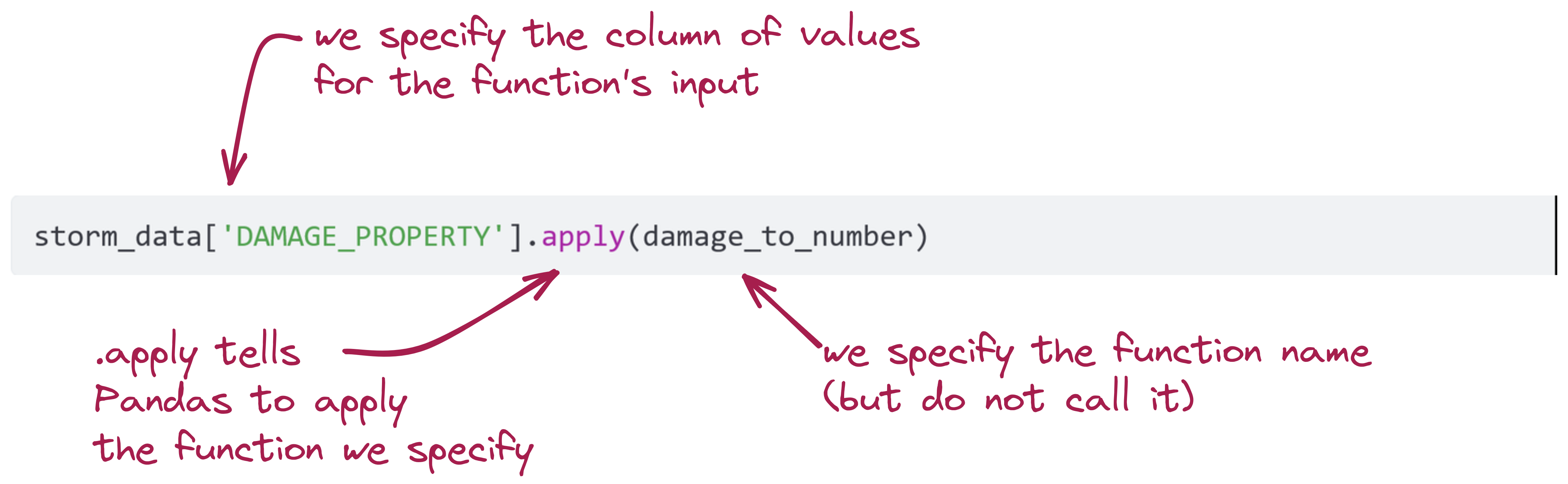
return damage_valueNow, we create a new column using our function using the apply function:
storm_data['DAMAGE_PROPERTY_VAL'] = storm_data['DAMAGE_PROPERTY'].apply(damage_to_number)
print(storm_data['DAMAGE_PROPERTY_VAL'])
0 0.0
1 0.0
2 0.0
3 0.0
4 50000.0
...
61380 0.0
61381 0.0
61382 5000.0
61383 0.0
61384 0.0
Name: DAMAGE_PROPERTY_VAL, Length: 61385, dtype: float64Let’s unpack the apply syntax:
Now let’s determine if the damage was greater than $25,000.
storm_data['EXPENSIVE'] = storm_data['DAMAGE_PROPERTY_VAL'] > 25000
print(storm_data['EXPENSIVE'].value_counts())
EXPENSIVE
False 58773
True 2612
Name: count, dtype: int64For very simple functions, we can simply use an operator with the column - just like with a Pandas Series!
For more complicated functions, we can write a function that operates on the entire row. What if we wanted to include crop damage?
First, we can could use our original function to convert the 'DAMAGE_CROPS' entries into floats:
storm_data['DAMAGE_CROPS_VAL'] = storm_data['DAMAGE_CROPS'].apply(damage_to_number)
print(storm_data['DAMAGE_CROPS_VAL'])
0 0.0
1 0.0
2 0.0
3 0.0
4 0.0
...
61380 0.0
61381 0.0
61382 0.0
61383 0.0
61384 0.0
Name: DAMAGE_CROPS_VAL, Length: 61385, dtype: float64This is a good example of how functions let us re-use our code for different applications.
Next, we can write a function that determines if either crop or property damage (or both!) was greater than $25,000:
def expensive_calc(row):
    property_expensive = row['DAMAGE_PROPERTY_VAL'] > 25000
    crops_expensive = row['DAMAGE_CROPS_VAL'] > 25000
    return property_expensive or crops_expensive
Finally, we apply it:
storm_data['EXPENSIVE'] = storm_data.apply(lambda row: expensive_calc(row), axis=1)
print(storm_data['EXPENSIVE'].value_counts())
EXPENSIVE
False 58536
True 2849
Name: count, dtype: int64The syntax here is a bit complicated:
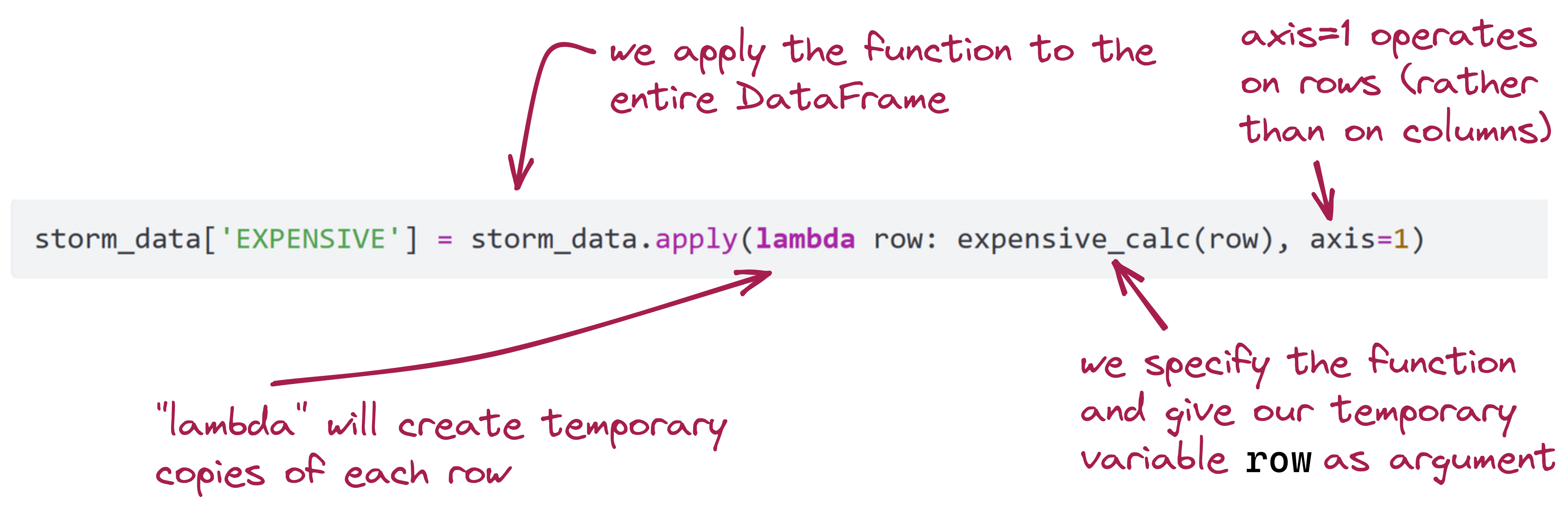
The complicated syntax has an upside: we can specify effectively any data manipulation we want using Python, Numpy and Pandas, and it scales to very large data sets.
Optional Multimedia Content (Another Red Panda Photograph)

(Image: Public Domain)
Exercise 2.1.5
2.1.5 - Plotting
While it is nice to be able to use value_counts() to print out information about the columns in a DataFrame, there are also extensive plotting libraries at our disposal that can generate more interesting and useful graphs.
We’re going to show a few simple examples with the plotting library Seaborn.
We’ll start by loading a simplified version of the dataset we’ve been using (damage_data.csv):
plot_data = pd.read_csv('damage_data.csv')
print(plot_data)
Unnamed: 0 State Month Damage
0 0 California Jan 2.241582e+08
1 1 California Feb 2.920000e+05
2 2 California Mar 1.780000e+05
3 3 California Apr 3.030000e+06
4 4 California May 1.150000e+04
.. ... ... ... ...
103 103 Louisiana Aug 1.215051e+10
104 104 Louisiana Sep 6.250000e+05
105 105 Louisiana Oct 3.552000e+06
106 106 Louisiana Nov 9.500000e+04
107 107 Louisiana Dec 9.500000e+04
[108 rows x 4 columns]You can see that the data consists of total damage for several states by month (it is for the year 2021).
We will start by using Seaborn to make a very simple line plot. Seaborn uses a similar import convention to Numpy and Pandas: import seaborn as sns.
import seaborn as sns
sns.set_style('dark')

ax = sns.lineplot(data=plot_data, x='Month', y='Damage')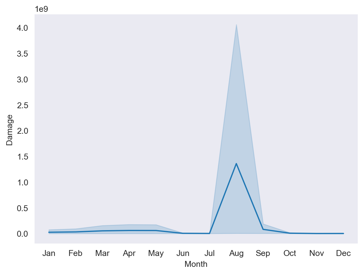
Important Notes for Thonny Users
Thonny is a convenient editor for learning basic Python, however it is not as well-suited for working with data and plotting as other editors.
If you are using Thonny, you will need to use some additional code:
import matplotlib.pyplot as plt # add this once for the program
import seaborn as sns
sns.set_style('dark')

ax = sns.lineplot(data=plot_data, x='Month', y='Damage')
plt.show() # add this every time you make a plot- You must add
import matplotlib.pyplot as pltonce at the beginning of the program - You must add
plt.show()whenever you display a graph
Of the tools we used in this class, Spyder is a better editor for graphs. No additional code is needed for your plots to show up in Spyder’s “plots” window.
- For projects after this class, you might want to try Jupyter Notebooks.
- If you installed Anaconda, you already have Jupyer Notebooks installed - you can run them from the Anaconda Navigator.
- Jupyter Notebooks do not use
.pyfiles. For this course, code you turn in must be a.pyfile.
- VS Code is another popular editor used by professional software engineers.
This simple line plot shows both an average value for the damage, as well as “error,” representing minimum and maximum values by state and month.
You can see that we used Seaborn’s sns.lineplot function, which takes several named arguments:
sns.set_style('dark')sets Seaborn’s plotting styledataspecifies a Pandas DataFramexspecifies the DataFrame column for the x-values (by string)yspecifies the DataFrame column for the y-values (by string)
You can also see that we assigned the plot’s output to a variable, ax. This is a convention that defines the plot on “axes,” which we can use later to change things about the plot.
Seaborn has a number of options for changing the plot’s style.
sns.set_style('whitegrid')
ax = sns.lineplot(data=plot_data, x='Month', y='Damage', linewidth=0.75)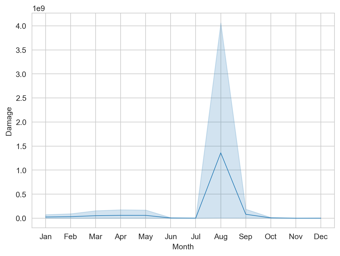
- One option called
sns.set_styleto apply a grid to the plot’s background - Another added a named argument to
sns.lineplot,linewidth, to change the line’s width
Now let’s change the scale and labels for the plot:
sns.set_style('whitegrid')
ax = sns.lineplot(data=plot_data,
                  x='Month',
                  y=plot_data['Damage']/(10**6),
                  linewidth=0.75)
ax.set(xlabel='Month',
       ylabel='Damage ($millions)',
       title='Damage per Month');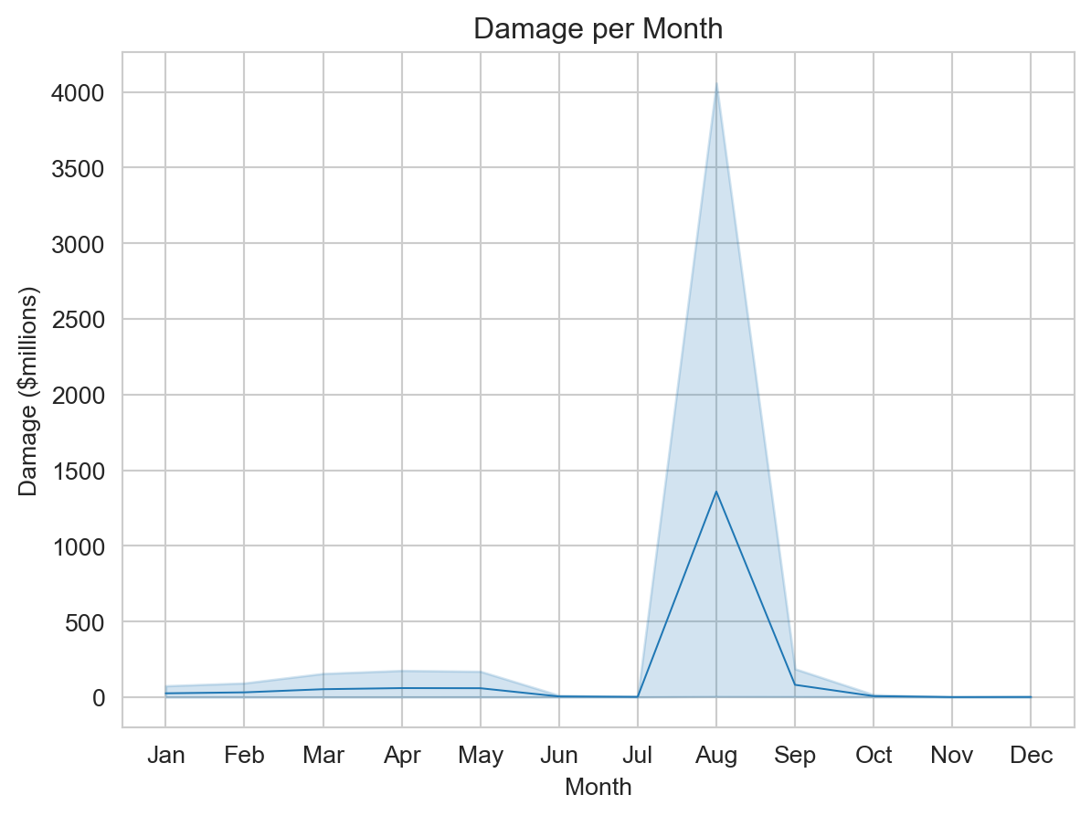
Note that we inserted some whitespace after the comma-separated arguments. Whitespace after commas in arguments, list items, dict entries, etc., is ignored, and can be used to organize your code.
Here’s what changed:
- The argument
ywas changed from a string to an explicit reference to the DataFrame- We call out
plot_data['Damage'] - We divide it by one million (\(10^6\), which is
10**6in Python)
- We call out
- We set the axes labels and title:
- Because we divided the damage value by 1000, we indicate that damage is now in thousands of dollars
- We added a title
Now let’s plot individual state damage data, all on one line plot:
sns.set_style('whitegrid')
ax = sns.lineplot(data=plot_data,
                  x='Month',
                  y=plot_data['Damage']/(10 ** 6),
                  hue='State',
                  linewidth=1.5)
ax.set(xlabel='Month',
       ylabel='Damage ($millions)',
       title='Damage per Month');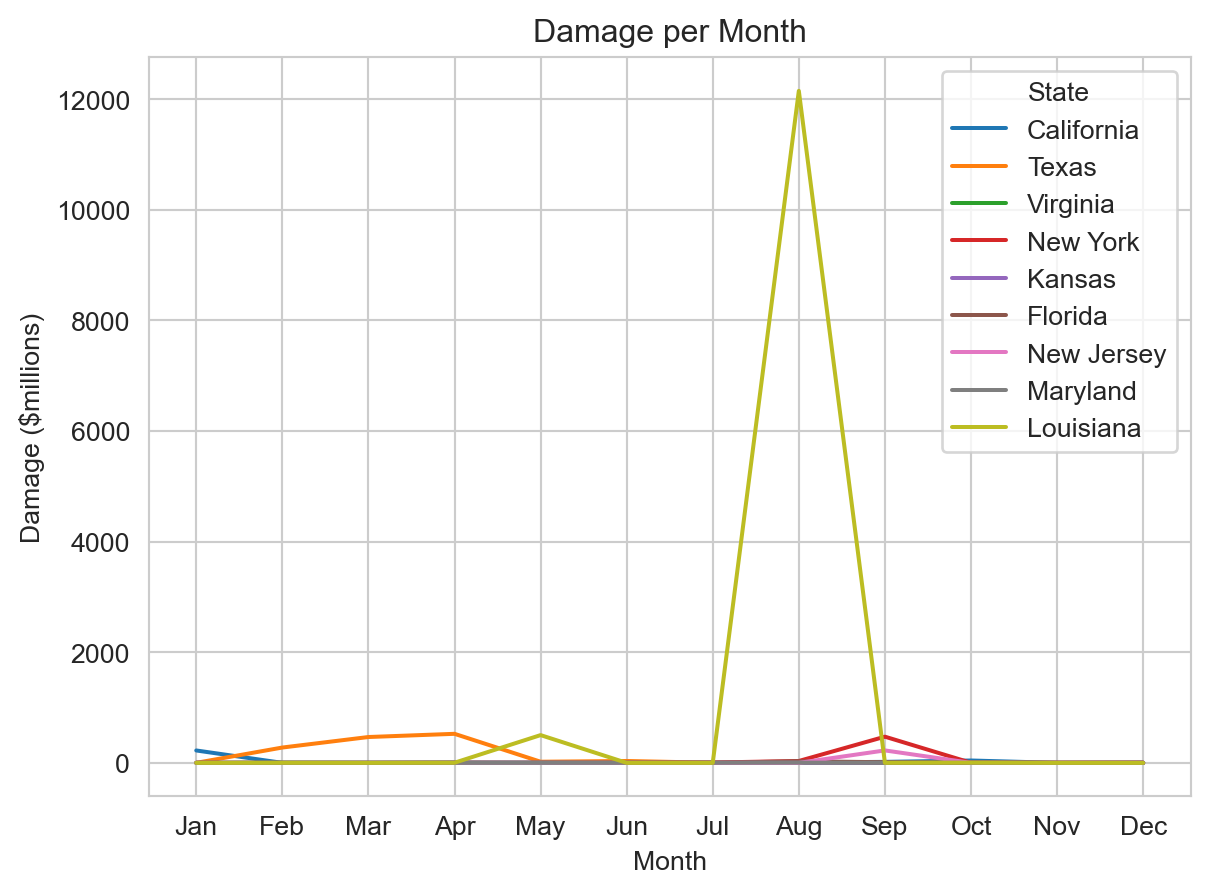
All we added was hue='State'. We can see how much Hurricane Ida (which made landfall in Louisiana in August 2021) dominates this data set.
Perhaps we want to be able to usefully see information about just the states other than Louisiana. We can use the DataFrame drop function to remove Louisiana and create a new DataFrame with just the other states.
plot_data2 = plot_data.drop(plot_data[plot_data['State'] == 'Louisiana'].index)

sns.set_style('whitegrid')
ax = sns.lineplot(data=plot_data2,
                  x='Month',
                  y=plot_data2['Damage']/(10 ** 6),
                  hue='State',
                  linewidth=1.5)
ax.set(xlabel='Month',
       ylabel='Damage ($millions)',
       title='Damage per Month');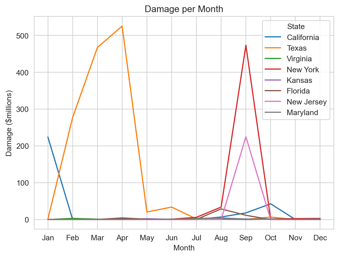
These are just a few things we can do, Seaborn has a lot of options for plots you can make - and you now know enough Python to read the documentation and learn more.
Exercise 2.1.5
2.1.6 - More Python Than You Require
You have now seen the basic syntax for using Python for numerical an data analysis, including making plots. There are many more kinds of analysis you can perform, and many more kinds of plots you can make.
- The documentation for Numpy and Pandas is very detailed, and explains how many of the functions (including numerous ones we have not used) work.
- For mathematical and scientific analysis, you may be interested in using SciPy - Scientific Python.
- Seaborn has tutorials for making various kinds of graphics.
- Matplotlib is another popular plotting library (that Seaborn uses, “under the hood”)
- We recommend using Jupyter Notebooks for data analysis and data science applications.
- The official Python documentation is very thorough, but not always easy to read.
Remember: writing some code to see what happens or trying some different things in Python and looking at the output is free. Playing with the programming language and making mistakes is a great way to learn more. You have reached the end of the course, but there’s a lot more Python out there, if you want it. Stay curious!
End-Of-Module Problems
There are no end-of-module problems for Module 2.1. Instead, complete the exercises in the module and submit them for credit.
That is all.