Module 1.4 - Numerical Processing and I/O
Objectives
By the end of this module you will be able to:
- Perform more advanced numerical processing using loops.
- Work through examples of using the
breakstatement. - Write code to read and write to text files.
1.4.0 Numerical Applications of Loops
There are several ways in which we’ll work with numbers and loops. The one is to use integers to drive the loop’s iterations as in:
for k in range(1, n):
    # do stuff
Here, k, 1, and n, are all integers. The second is more advanced in that real numbers can themselves be used in the range. We’ll tackle this approach later but we’ll give you a preview of what it looks like:
import numpy

for r in numpy.arange(0.1, 1, 0.2):
    # do stuff
Let’s start with an example:
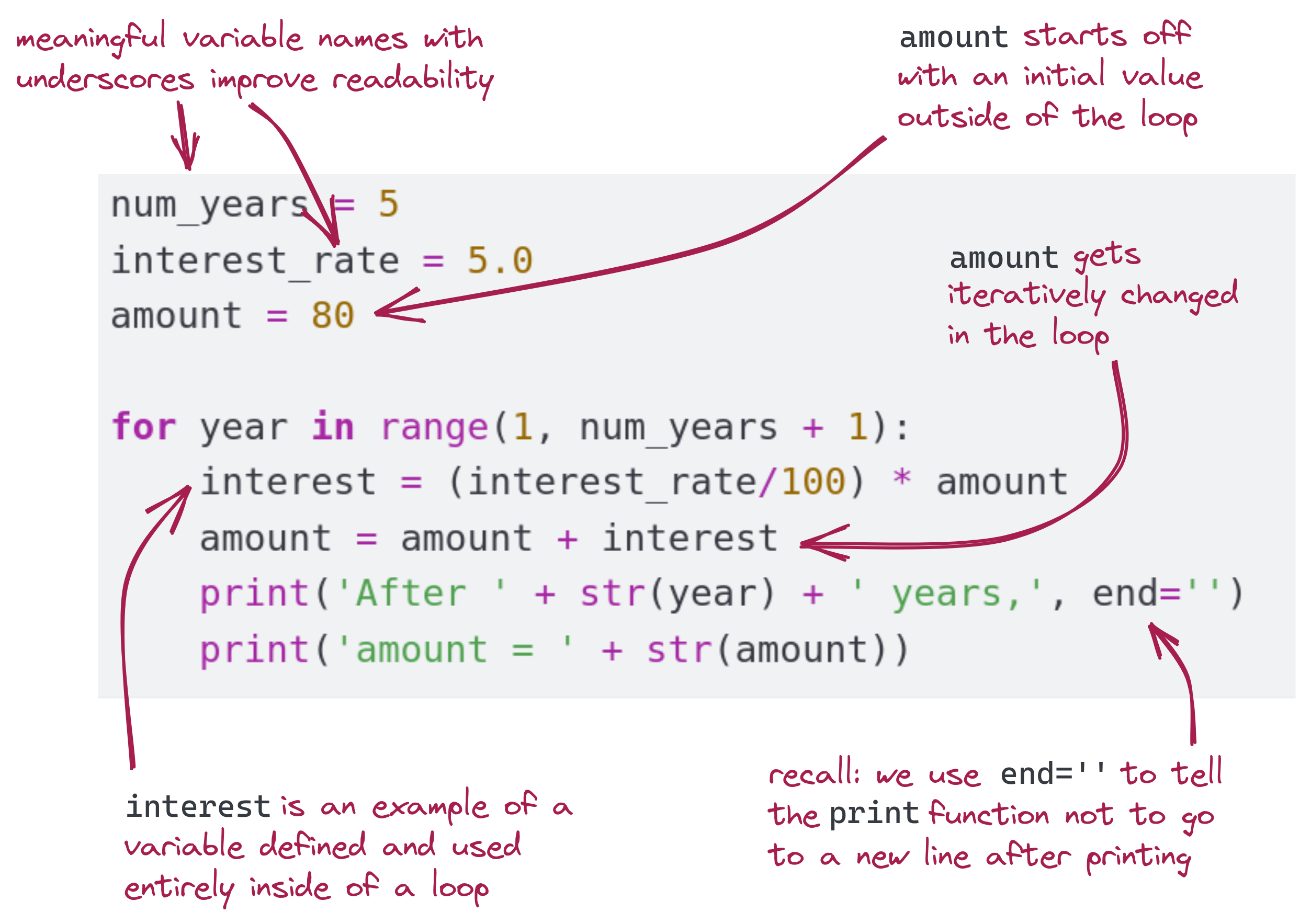
num_years = 5
interest_rate = 5.0
amount = 80

for year in range(1, num_years + 1):
    interest = (interest_rate/100) * amount
    amount = amount + interest
    print('After ' + str(year) + ' years,', end='')
print('amount = ' + str(amount))- Trace through the iterations above using a table, tracking the variables
year, amount, interest.
Exercise 1.4.1
Let’s point out:
Exercise 1.4.2
1.4.1 A Statistical Application
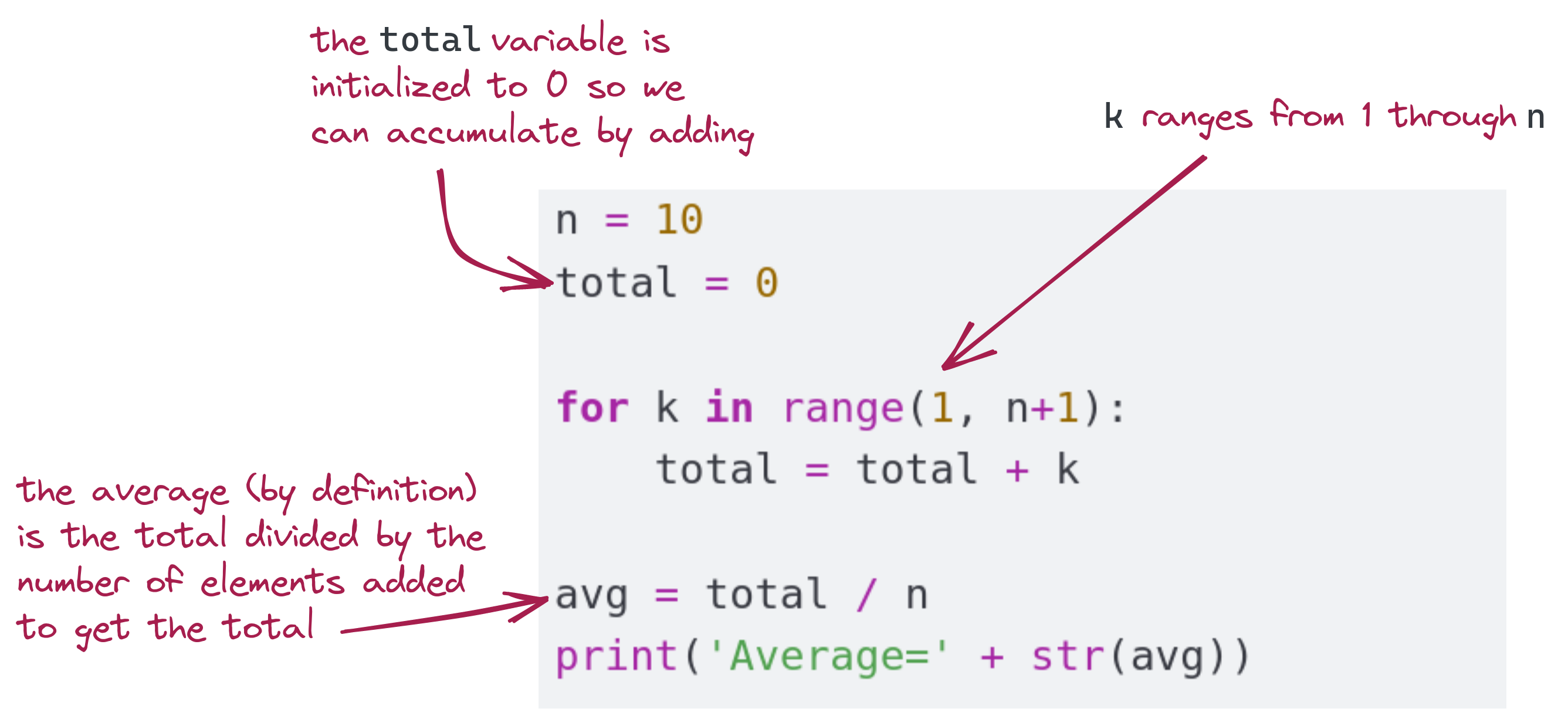
Let’s use a loop to compute a basic statistical quantity: an average (arithmetic mean). For example, suppose we wish to compute the average of the numbers from 1 to 10:
n = 10
total = 0

for k in range(1, n+1):
    total = total + k

avg = total / n
print('Average=' + str(avg))
Note:
Exercise 1.4.3
Exercise 1.4.4
1.4.2 Plotting a Function
Let’s plot the well-known \(\sin\) function.
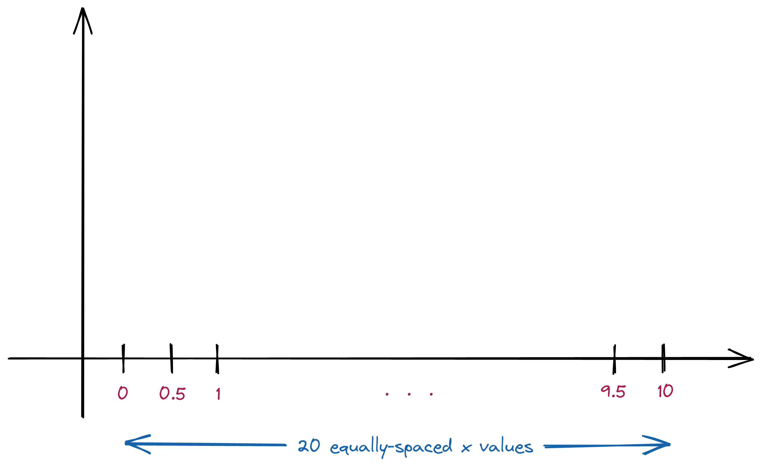
- We’ll plot this in the range \([0,10]\).
- Let’s start by picking 20 points to plot.
- We’ll divide the interval into 20 so that the values (along the x-axis) are:
0
0.5
1.0
1.5
... (20 equally spaced values along x-axis)
9.5
10.0
Pictorially, this is what we’ve done so far:
Then, the y-values are calculated by applying the function:
f(0)      = sin(0)      =  0
f(0.5)    = sin(0.5)    =  0.48
f(1.0)    = sin(1.0)    =  0.84
f(1.5)    = sin(1.5)    =  0.997
...
f(9.5)    = sin(9.5)    = -0.075
f(10.0)   = sin(10.0)   = -0.54
For now, don’t worry about the meaning of this \(\sin\) function. - Just think of it as: you give it a value like 0.5, and it gives back a number like 0.005. - We’ll say more about this below.
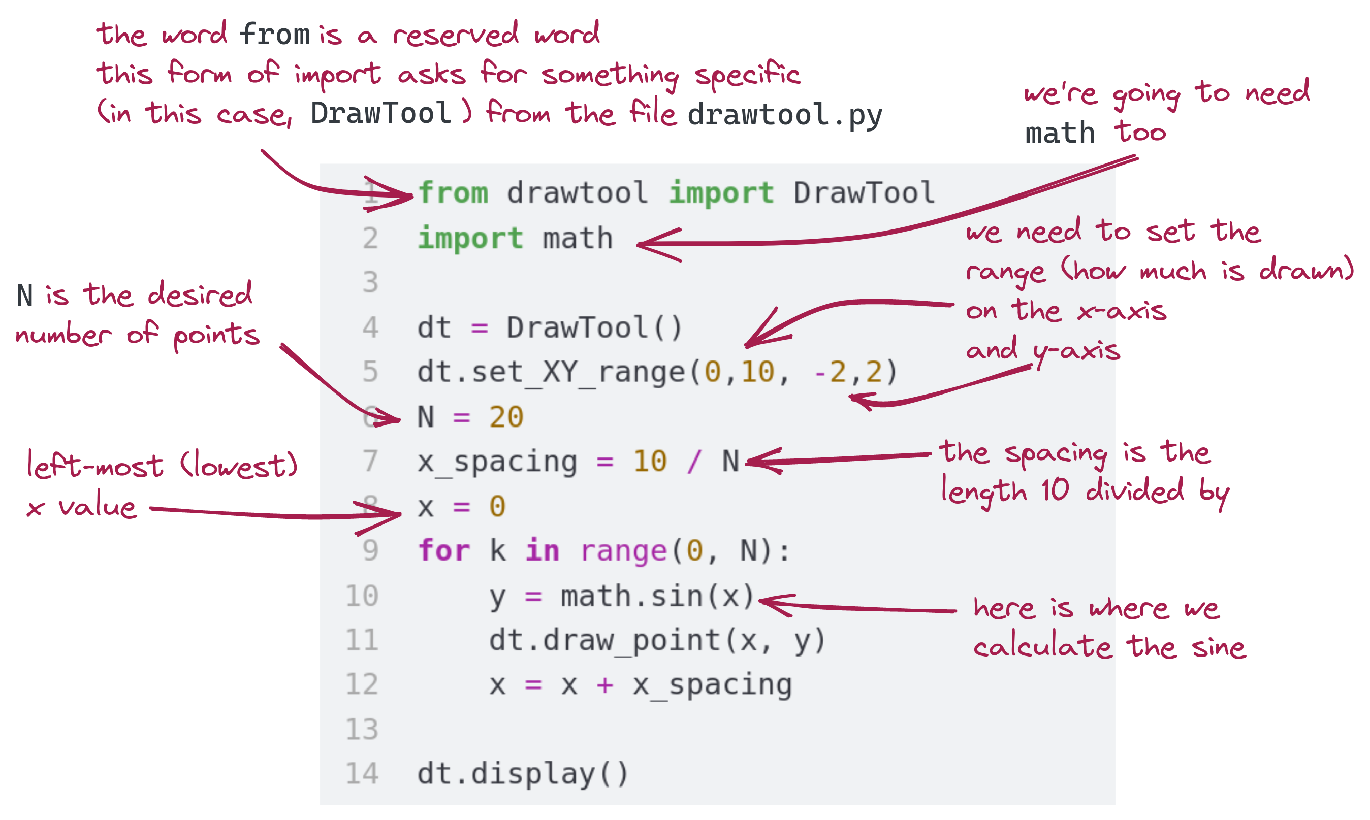
Let’s do the plotting in code:
from drawtool import DrawTool
import math

dt = DrawTool()
dt.set_XY_range(0,10, -2,2)
N = 20
x_spacing = 10 / N
x = 0
for k in range(0, N):
    y = math.sin(x)
    dt.draw_point(x, y)
    x = x + x_spacing

dt.display()
Exercise 1.4.5
Let’s point out:
Note: Much of the complication in this program comes from how we use another program in our program: To perform plotting or drawing, we will use the drawtool.py program.
To use this program involves many types of statements, such as:
dt = DrawTool()
dt.set_XY_range(0,10, -2,2)
among others.
- There are aspects we’re not going to be able to understand now, but we can at least use the program. Notice that when N=20, the spacing is 10/20 (which is equal to 0.5).
- If a higher value of N were used, we’d have smaller spacing and therefore a smoother curve.
About mathematical functions:
- The term function means different things in programming and math. For us in programming, a function is a chunk of code that can be referenced by a name and used multiple times just by using that name.
- In math, a function is a calculation mechanism, which we can think of as “something that takes in a number and outputs a number via a calculation:””
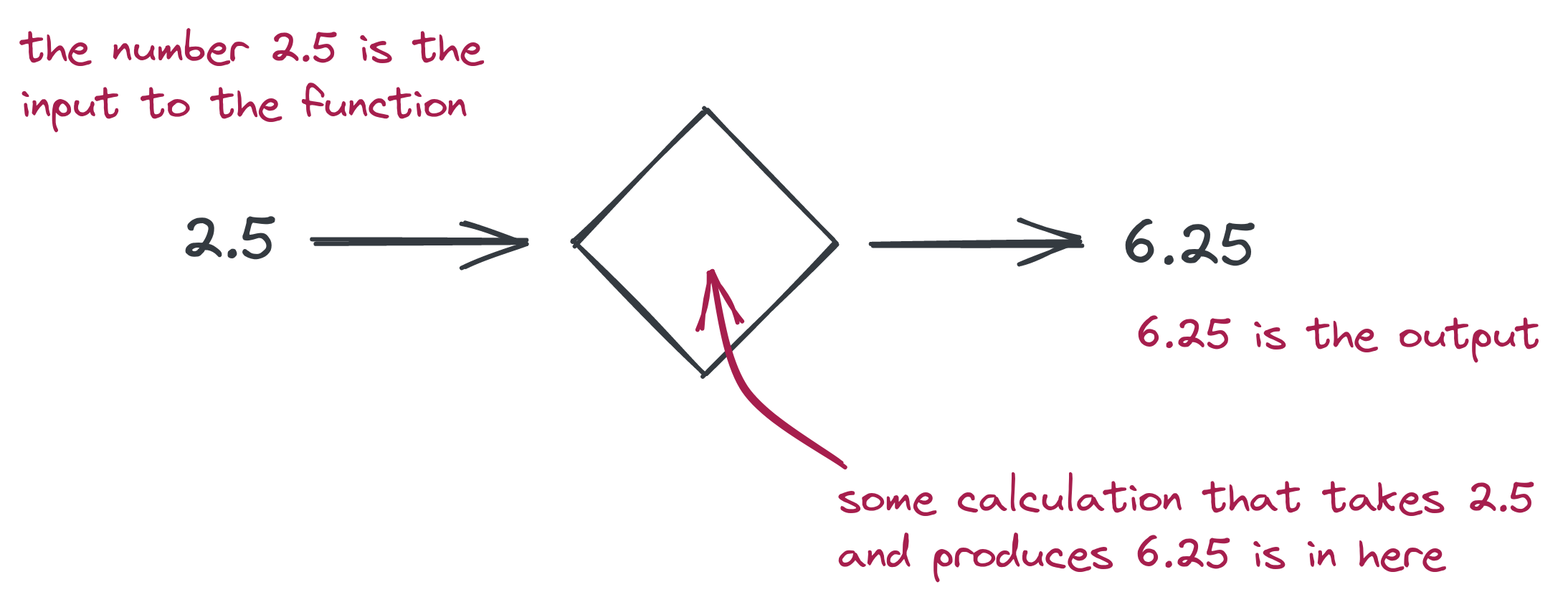
For example:
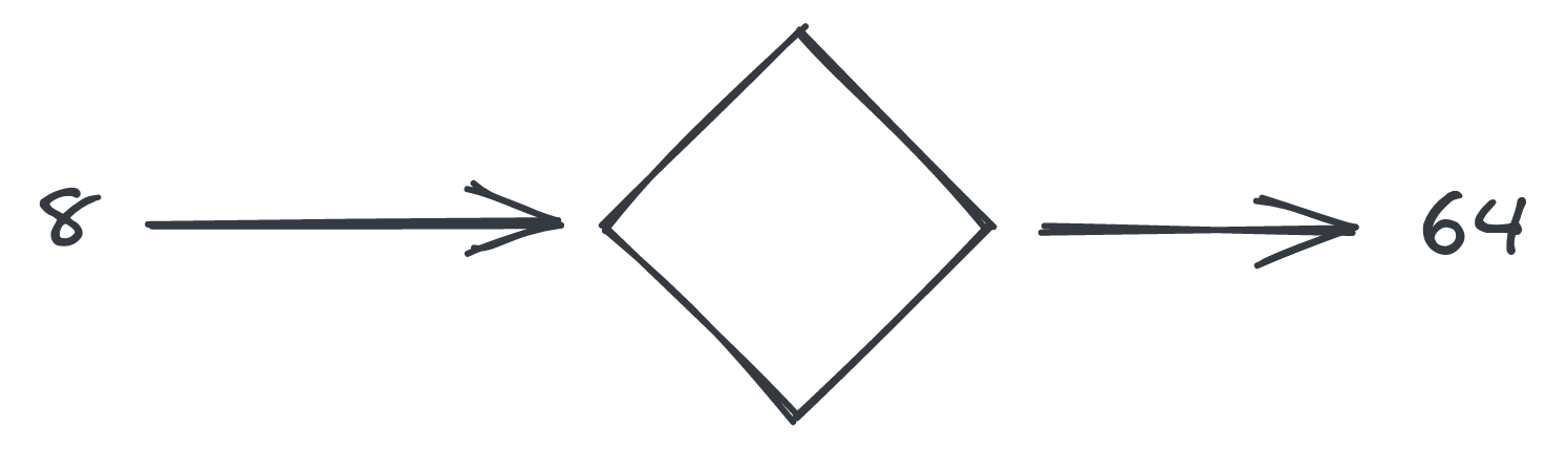
- In this particular case, suppose we feed in 8, we get 64
- The rule that turns the input number into the output number is: multiply the input number by itself.
- Thus: \(8^2 = 64\) To describe this in a simpler way, we use symbols like \(x\)
- And instead of drawing boxes, we use mathematical notation like this: \(f(x) = x^2\).
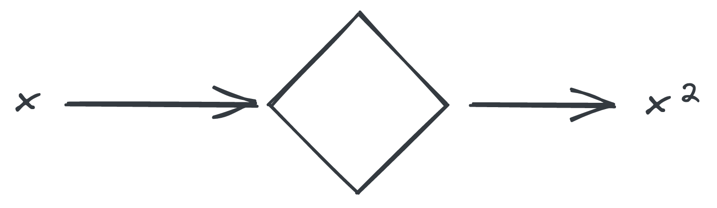
- Read this as: the function takes in a number \(x\) and produces \(x^2\). There are many common functions, amongst these are the trigonometric functions like \(\sin\). Thus, \(\sin(x)\) takes in a number \(x\) and produces a number \(sin(x)\) as a result.
In the early 1600’s Rene Descartes made a startling discovery that dramatically changed the world of math:
- You can make axes.
- For every possible \(x\) you can compute \(f(x)\)
- Then draw each pair \(x,f(x)\) as a point. This produces a curve that allows one to visualize a function.
- This is what we did when we plotting the \(\sin\) function.
About the \(\sin\) function:
- You may vaguely recall trigonometry from high-school, or have happily forgotten it.
- Perhaps you recall triangles and ratios of sides. The \(\sin\) function arose from those ideas.
- This is more than a textbook exercise, functions like \(\sin\) have proven extraordinarily useful both in real-world applications and in pure mathematics.
- We’re not going to require much math knowledge in this course, but we will make observations from time to time.
1.4.3 Plotting a Curve With Data
Next, let’s work with some real data.
Consider the following data:
| \(x\) | \(f(x)\) |
|---|---|
| 8.33 | 1666.67 |
| 22.22 | 3666.67 |
| 23.61 | 4833.33 |
| 30.55 | 5000 |
| 36.81 | 5166.67 |
| 47.22 | 8000 |
| 69.44 | 11333.33 |
| 105.56 | 19666.67 |
Let’s write code to display this data:
from drawtool import DrawTool
import math

dt = DrawTool()

dt.set_XY_range(0,120, 0,20000)

x = 8.33
f = 1666.67
dt.draw_point (x, f)

x = 22.22
f = 3666.67
dt.draw_point (x, f)

x = 23.61
f = 4833.33
dt.draw_point (x, f)

x = 30.55
f = 5000
dt.draw_point (x, f)

x = 36.81
f = 5166.67
dt.draw_point (x, f)

x = 47.22
f = 8000
dt.draw_point (x, f)

x = 69.44
f = 11333.33
dt.draw_point (x, f)

x = 105.56
f = 19666.67
dt.draw_point (x, f)

dt.display()
Exercise 1.4.6
1.4.4 Using break in Loops
As an example, let’s write a program to find the largest square that’s less than 1000.
Here’s the code:
k = 1
while k*k < 1000:
    k = k + 1

k = k - 1
print('largest square < 1000:', k*k, '= square of', k)
One can use a break statement as an alternative to writing the “loop exit” condition as the while condition. We’ll first do this with a for loop, and then see something unusual with the while loop version.
To simplify tracing, let’s rephrase to “largest square less than 50”.
First, the for loop version:
for k in range(1, 50):
    # print('Before-if: k =', k)
    if k*k > 50:
        break
    # print('After-if: k =', k)

k = k - 1
print(k)
Exercise 1.4.7
- A
breakstatement is the reserved wordbreakall by itself on a line, as seen above. When abreakstatement executes, Python looks for the loop that encloses the break and abruptly exits the loop without running any more code.breakstatements are useful to check for conditions that should result in leaving the loop immediately. One could write code like this, but it would make no sense:
for k in range(10):
    print(k)
    break
This would cause the first value (0) to print and then break out of the loop. As a mathematical aside, we know that we don’t really need the for loop range to be as high as 50. After all, as k gets close to 50, there is no way k*k would be less than 50. However, we’ll leave it as is, for the sake of simplicity.
There are options in writing the loop. Consider this one:
for k in range(1, 50):
    if (k+1)*(k+1) > 50:
        print(k)
        break
Is this more elegant, if a bit harder to understand at first?
Exercise 1.4.8
Next, let’s look at a while loop version of the original (using 50 instead of 1000)
Here’s the code:
k = 1
while True:
    if k*k > 50:
        break
    k = k + 1

k = k - 1
print(k)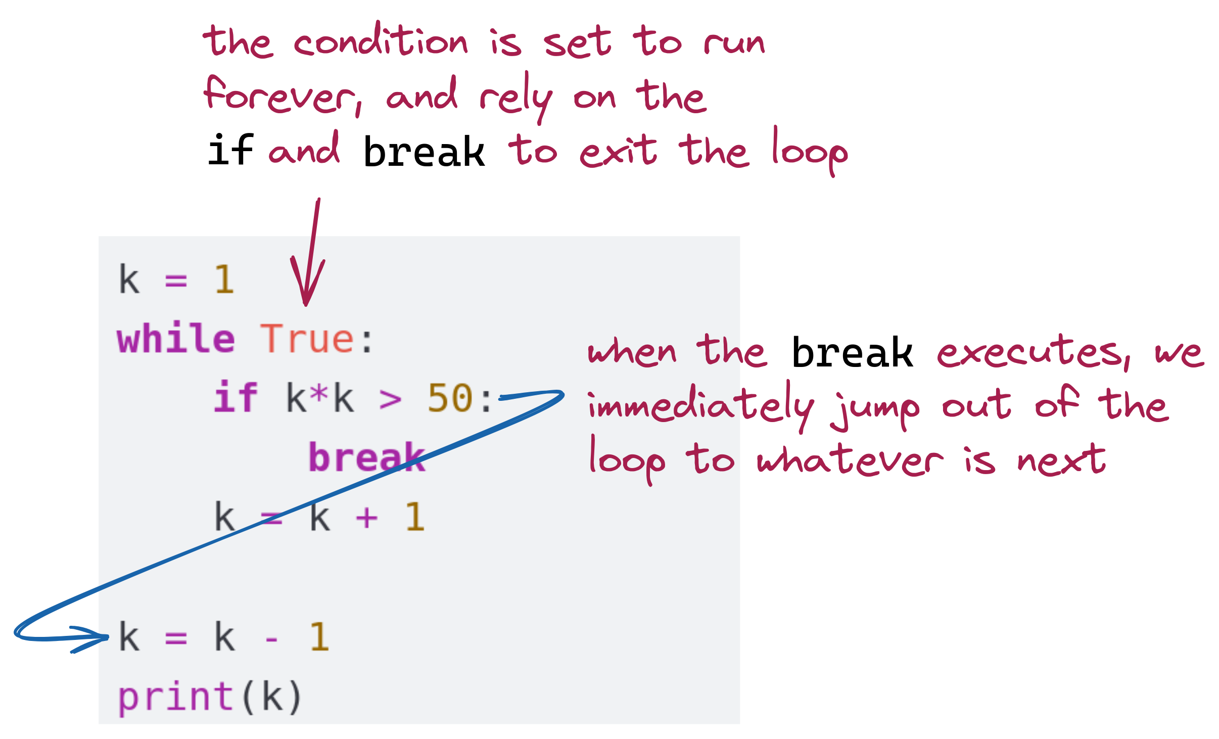
- Was it surprising that we deliberately set up a loop to appear to run forever?
- This is valid and often desirable, provided we are careful to set up a condition inside the loop to break out eventually.
- We need to be sure we hit that condition eventually.
Exercise 1.4.9
Exercise 1.4.10
1.4.5 More Probability and Statistics
Consider the following problem:
- An experiment consists of flipping three coins.
- The experiment is repeated until all three are “heads”
- On average, how many experiments are needed until all three turn up “heads”?
One way to think about this problem “statistically” is this:
- Suppose we hire a thousand people to each perform repeated three-coin flips.
- For very few of these people, they’ll get “heads-heads-heads” the very first experiment.
- For others, they might have to repeat many times before they see this.
- Each person counts how many experiments had to be tried before getting three-heads. The result is the average number across the thousand people: the average number of 3-coin flips needed to see three heads.
Instead of calculating by hand, we will write a program to estimate this number:
import random

num_trials = 1000
total = 0

for k in range(num_trials):
    got_three = False
    num_three_flips = 0
    while not got_three:
        c1 = random.choice(['H','T'])
        c2 = random.choice(['H','T'])
        c3 = random.choice(['H','T'])
        num_three_flips += 1
        if (c1 == 'H') and (c2 == 'H') and (c3 == 'H'):
            got_three = True
    total += num_three_flips

estimate = total / num_trials
print('Estimate: ', estimate)
Exercise 1.4.11
Let’s look at the general process of estimation (the outer loop) that we’d use in any estimation problem:
num_trials = 1000
total = 0

for k in range(num_trials):
    # for a successful trial, add 1 to the total

estimate = total / num_trials
Now let’s look inside to see how each trial is performed:
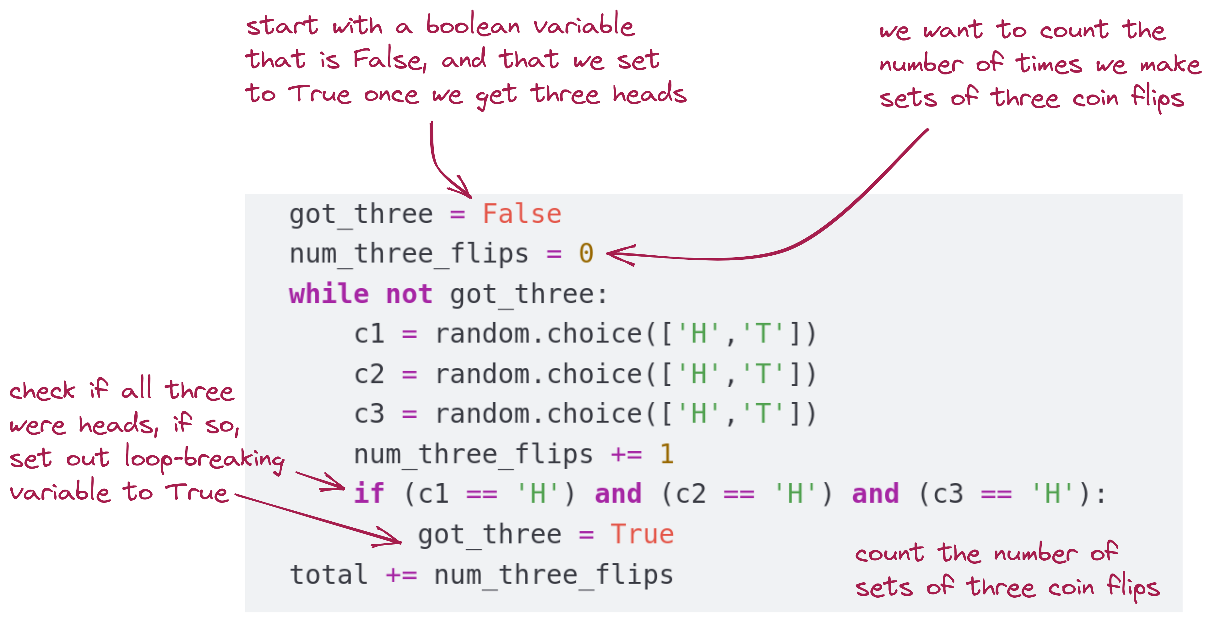
A variable like got_three is sometimes called a flag variable: we use it to flag a condition that we’re looking for.
Exercise 1.4.12
Exercise 1.4.13
1.4.6 Reading From a File
Very often, data is collected and stored in files, and so it’s useful to write code that reads data out of files.
Let’s start with a simple test file of plain text. First, examine the file testfile.txt to see that it’s a file consisting of four lines of text.
(From the poet Ogden Nash.)
We will look at a few different versions of reading from this file.
Here’s the first:
with open('testfile.txt', 'r') as in_file:
    lines = in_file.read()

print(type(lines))
print(lines)
Exercise 1.4.14
Notes:
- We’ve used two Python reserved words:
withandas. Although file input/output (I/O) does not strictly require thewithstructure, it is useful because:- Files that are being accessed by one program are said to be in an “opened” state.
- For another program to be able access the file, the first one has to “close” it (that is, signal that it’s done with the file).
- The
withstructure automatically takes care of this.
- The function call to
opentakes the name of the file and the kind of access, for example:with open('testfile.txt', 'r') as in_file:
'r'for read-only access (we’re not changing the file here)'w'for write, if we should choose to. The result of opening a file is to get a special kind of variable, what we’ve calledin_filein this case:with open('testfile.txt', 'r') as in_file:- It is this variable that’s going to perform the reading and, in this case, get us all the text in one shot:
lines = in_file.read() - Note that all the lines are returned as a single string. This means, it will be difficult to analyze line-by-line, if that’s our goal.
- It is this variable that’s going to perform the reading and, in this case, get us all the text in one shot:
- There is a way to take the single string and break it into separate lines, but let’s instead find a way to read separate lines.
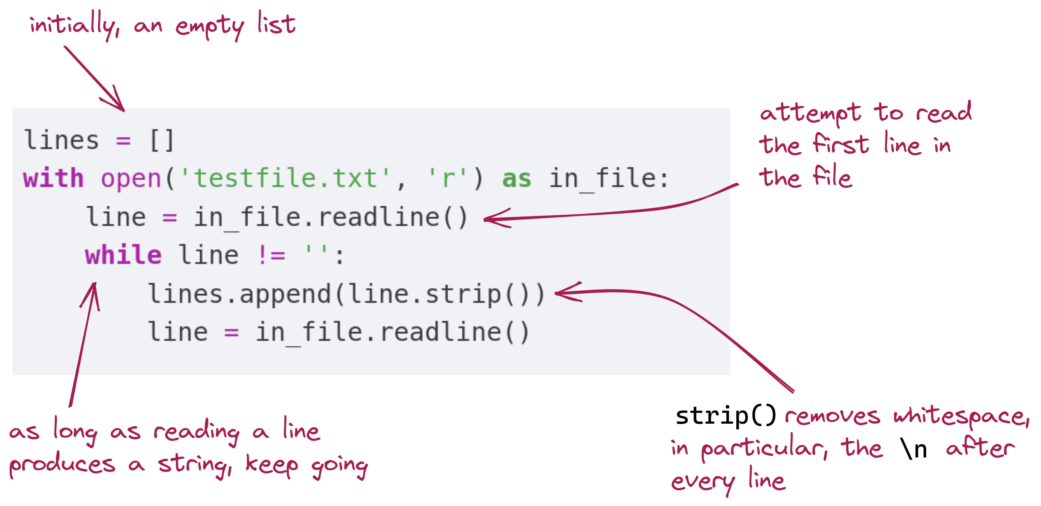
Accordingly, let’s look at a way to read the file into a list of strings, where each line is one string in the list:
lines = []
with open('testfile.txt', 'r') as in_file:
    line = in_file.readline()
    while line != '':
        lines.append(line.strip())
        line = in_file.readline()

print(type(lines))
print(lines)
Exercise 1.4.15
Notes:
- Here, we’re reading one line at a time and appending to a running list, which is the
linesvariable. - The problem is, for any general file, we won’t know in advance how many lines of text are in the file.
- A
whileloop to the rescue! Thus, we keep reading from the file as long as a read operation produces a line:
Writing to a file: Suppose we’ve read a text file into a list of strings. Let’s now write these to a new file.
with open('testcopy.txt', 'w') as out_file:
    for line in lines:
out_file.write(line + '\n')- This time, we’re opening a file called
testcopy.txtfor the purpose of writing to it - We’ve named our file variable
out_file. That will let us use a function calledwrite() - Here, we’re looping through the list, writing each string as one line in the file. Notice that we need to insert the
'\n'at the end of each line. '\n'represents an instruction to both output and files to “go to the next line”.
For example
print('hello' + 'world')           # Prints helloworld on one line
print('hello' + '\n' + 'world') # Prints "hello" and prints "world" on the next line- So, to write strings to different lines, we have to tell the function that writes to files to go to the next line with an explicit
'\n'. It’s similar with reading, if we read a whole file as one string, that string will contain the linebreaks (the ‘’ characters).
Exercise 1.4.16
Next, let’s read from a file of numbers and perform some basic stats: First, examine the file data.txt and see that it’s a collection of numbers, one per line. We’ll read line by line as a string, and then convert to a floating-point number:
data = []
with open('data.txt', 'r') as in_file:
    line = in_file.readline()
    while line != '':
        s = line.strip()           # Remove leading/trailing whitespace
        x = float(s)               # Convert string to float
        data.append(x)             # Add to our list
        line = in_file.readline()  # Get the next line

print(data)
Exercise 1.4.17
1.4.7 Extracting Multiple Data From Each Line
Consider a data file that looks like this, with three numbers on each line:
6.0 6.0 9.0
4 6 8
24   16 2
 3 3.0 3
0.1 0.5 0.3
What we’d like to do is compute the average of the numbers in each line. So, the output should be something like:
Average of 6.0 6.0 9.0 is: 7.0
Average of 4.0 6.0 8.0 is: 6.0
Average of 24.0 16.0 2.0 is: 14.0
Average of 3.0 3.0 3.0 is: 3.0
Average of 0.1 0.5 0.3 is: 0.3
Therefore, what we need to do is not only read a line at a time, but be able to extract multiple items from within a line.
We can split a string as follows: Consider this example:
s = '6.0 6.0 9.0'
data = s.split()    # data is a list
print(data)
Here, the split() function in strings, looks for whitespace within and separates out into a list those items separated by this whitespace. So, in the above example, we’ll have the string '6.0 6.0 9.0' split into a list of three strings ['6.0', '6.0', '9.0']
Having a list of strings is not enough to compute the average of the numbers in those strings. We need to convert into numbers:
s = '6.0 6.0 9.0'
data = s.split()    # data is a list
print(data)
x = float(data[0])
y = float(data[1])
z = float(data[2])  # x, y, z are numbers
avg = (x + y + z) / 3.0
print(avg)- We can now read one line at a time from the data file, split each line, convert to numbers, and then calculate the average for each line.
Exercise 1.4.18
- We’ll now tackle one additional complication: it is common for real data to be acquired or presented with mistakes, missing entries, or inconsistent whitespace.
- The missing entry problem is somewhat harder to tackle, so we’ll postpone that for another time.
- But we can easily eliminate whitespace using the
strip()function.
For example, consider:
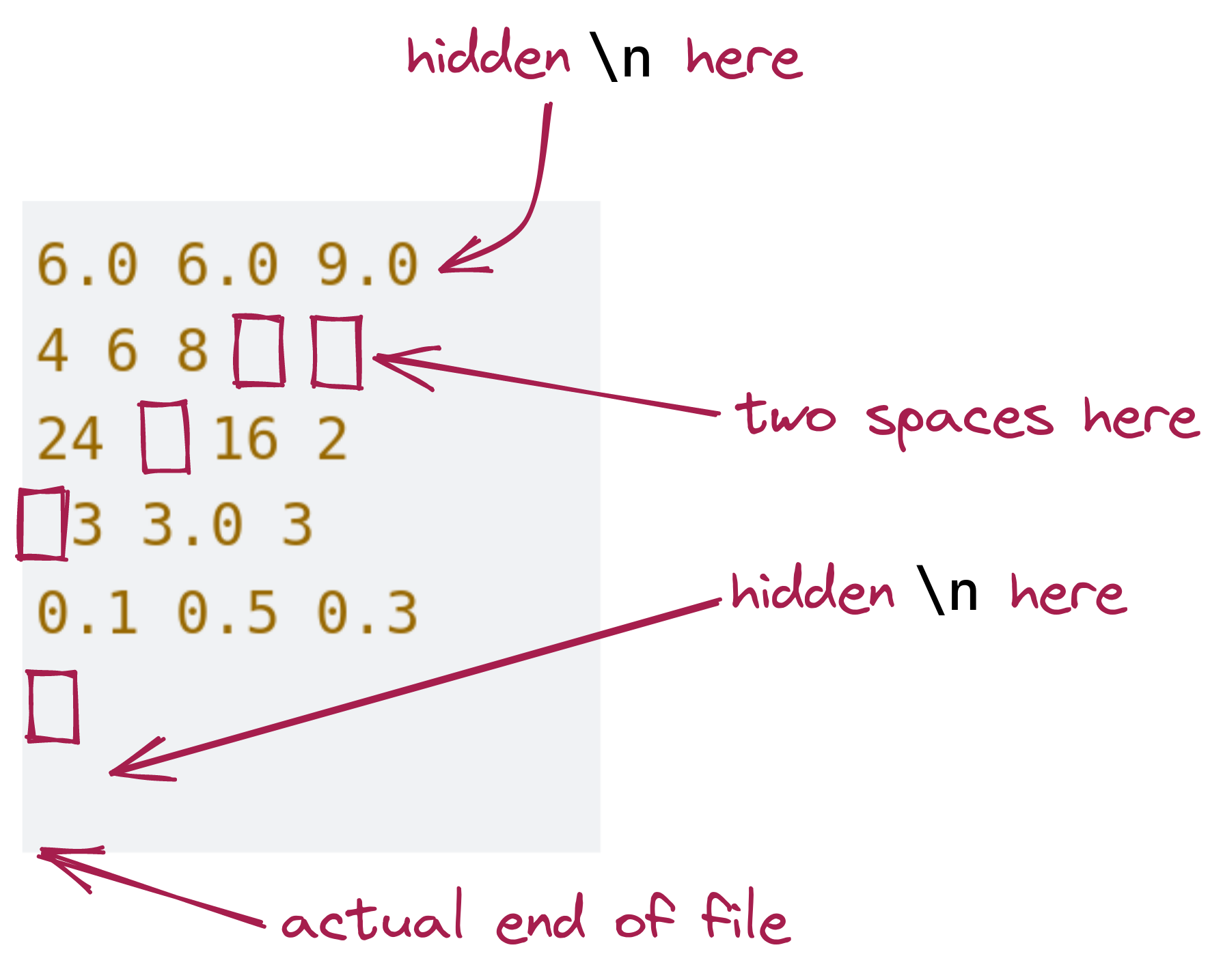
Thus, we need to worry about when a line is all whitespace but not empty. Let’s put these ideas into code:
with open('data2.txt','r') as in_file:
    line = in_file.readline()
    while line != None:
        line = line.strip()
        print('[', line, ']', sep='')
        if len(line) == 0:
            break
        data = line.split()
        print(data)
        x = float(data[0])
        y = float(data[1])
        z = float(data[2])
        avg = (x + y + z) / 3.0
        print('Average of ', x, ' ', y, ' ', z, ' is: ', avg, sep='')
        line = in_file.readline()
Exercise 1.4.19
We’ll point out a few things:
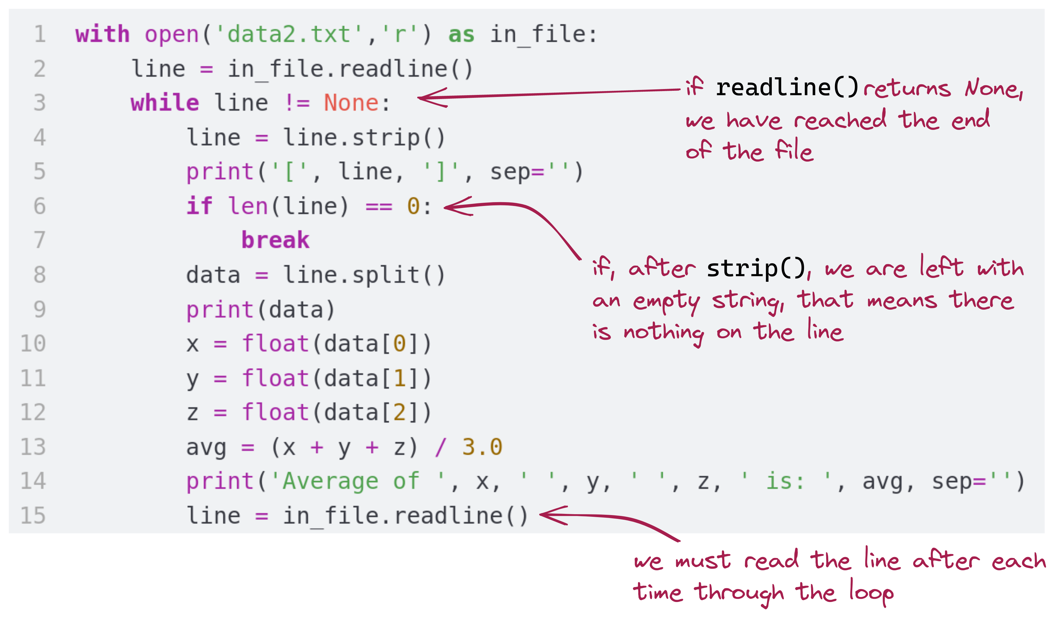
We have two print statements to see what we get as a result of strip() and split():
line = line.strip()
        print('[', line, ']', sep='')

        data = line.split()
print(data)- Recall: the
sep=''(empty separation) parameter tellsprint()not to add its own whitespace between different arguments. - Notice also that we have deliberately added in our printing, a pair of brackets:
print('[', line, ']', sep='')- This is a common programming technique when you want to identify whitespace: put something around it that is actually visible.
- You also noticed that
split()produces a list, and that each string in the list has already had whitespace removed on either side.
1.4.8 while Loops When Files Are Large
Let’s return to a problem we’ve seen before: identifying the longest sentence in a text file. Take a moment to review that section
- To find the longest sentence, we read the whole file into one giant list of sentences.
- We went through the list, recording the longest sentence.
- For a very large text file, the list could be too long to fit into memory.
- Let’s use a different version that reads sentence-by-sentence:
import wordtool as wt

def get_longest_sentence(filename):
    # Initiate the reading of the file
    sentences = wt.open_file_bysentence(filename)
    maxL = 0

    # Get first sentence
    s = wt.next_sentence()
    while s != None:
        if len(s) > maxL:       # Possibly update maxS
            maxL = len(s)
            maxS = s
        s = wt.next_sentence()  # next one

    return maxS

book = 'federalist_papers.txt'
s = get_longest_sentence(book)
print('Longest sentence in', book, 'with', len(s), 'chars:\n', s)
Exercise 1.4.20
1.4.9 Random Walks
We’re going to combine while loops with randomness and graphing. We will use a concept called a random walk:
- Imagine standing at the origin:
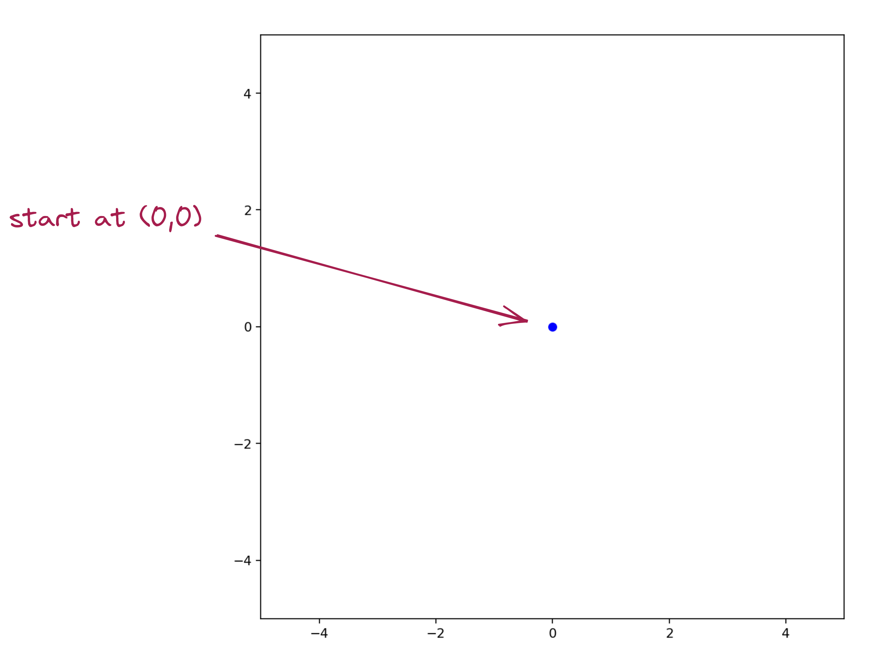
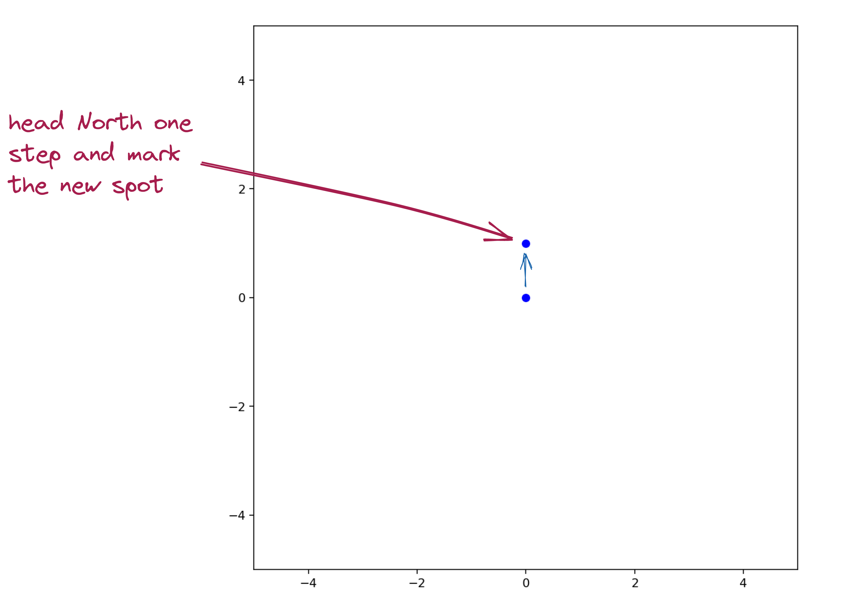
- Then, we choose a random direction from among: North, South, East, West.
-Once such a direction is randomly chosen: we take a fixed-size step in that direction, and mark the spot:
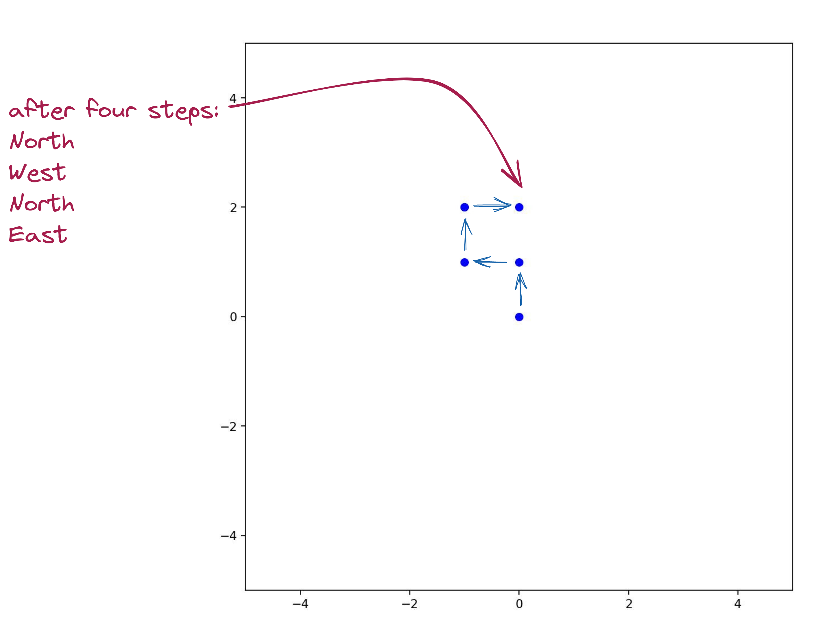
Here’s what it might look like after 4 steps:
Here’s the program:
import random
from drawtool import DrawTool

dt = DrawTool()
dt.set_XY_range(-5,5, -5,5)
dt.set_aspect('equal')

step = 1


def do_walk(max_steps):
    x = 0
    y = 0
    num_steps = 0
    dt.draw_point(x, y)
    while num_steps < max_steps:
        direction = random.choice(['N','S','W','E'])
        if direction == 'N':
            y += step
        elif direction == 'S':
            y -= step
        elif direction == 'E':
            x += step
        else:
            x -= step
        dt.draw_point(x, y)
        print(direction, x, y)
        num_steps += 1

do_walk(5)

dt.display()
Exercise 1.4.21
Instead of running the random walk for a fixed number of steps, we’ll now run the random walk until it “hits” one of the sides and stop. To do this, we’ll use the approach of:
 while True:
        # get a random direction and move
# if we hit one of the sides, then **break** - We’ll also enlarge the box to be bigger and make the step size smaller (so as to fill the space with dots).
Exercise 1.4.22
We’re now finally ready for the art project:
- We’ll start different random walks at randomly selected starting points, and then draw each in a random color.
Exercise 1.4.23
About random walks (in science): Random walks have had significant scientific impact. For example, a version of random walk is the basis for modeling diffusion and osmosis . The same basic idea underlies Brownian motion, Einstein’s demonstration of the existence of molecules, and the variation of stock prices. A random walk on networks (as opposed to 2D space) is what launched Google. Evolution is often modeled as a random walk on an abstract representation of the space of DNA sequences.
1.4.10 When Things Go Wrong
In each of the exercises below, first try to identify the error just by reading. Then type up the program to confirm, and after that, fix the error.
Exercise 1.4.24
Exercise 1.4.25
Exercise 1.4.26
End-Of-Module Problems
Full credit is 100 pts. There is no extra credit.
Problem 1.4.1 (100 pts)
Problem 1.4.2 (100 pts)
You may need to use this syntax to open a file, depending on your computer. Try it if you get encoding errors.
with open(fileName, 'r', encoding='utf-8') as f:
# file read operations- It adds the argument
encoding='utf-8'to theopenfunction. - Here,
fileNameis a string, representing the path to the file. If the file is in the same directory, it will simply be the file name.