A = [ [ [1,2], [3,4], [5,6] ], [ [7,8], [9,10], [11,12] ] ]
print(A[0])[[1, 2], [3, 4], [5, 6]]The goal of this module is to introduce numpy arrays, for use when working with numeric data.
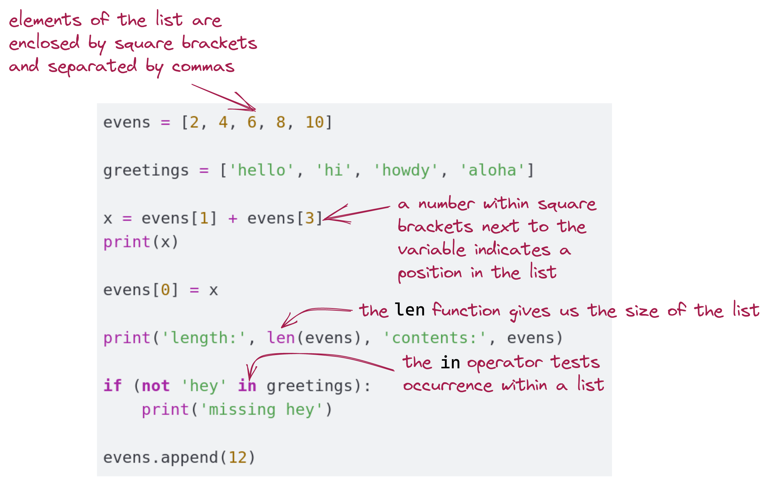
Recall a basic list:
# A list of integers:
evens = [2, 4, 6, 8, 10]

# A list of strings:
greetings = ['hello', 'hi', 'howdy', 'aloha']

# Access list elements using square brackets and index
x = evens[1] + evens[3]
print(x)

# We can change the value at an individual position
evens[0] = x

# Recall: len() gives us the length of the list
print('length:', len(evens), 'contents:', evens)

# Example of using **in** to search inside a list:
if (not 'hey' in greetings):
    print('missing hey')

# Add something new to the end of a list
evens.append(12)

# Write code here to increment each element by 2

print(evens)
# Should print: [12, 4, 6, 8, 10, 12] Let’s recall a few things we learned about lists via this example:
Why are lists useful? - Using a loop to create elements, as in:
for i in range(1, 10, 2):
A.append(2*i)for i in range(len(A)):
A[i] = 2 * A[i]for i in range(len(A)):
B[i] = A[i] + 5Lists allow both index iteration as above but also content iteration:
total = 0
for k in A:
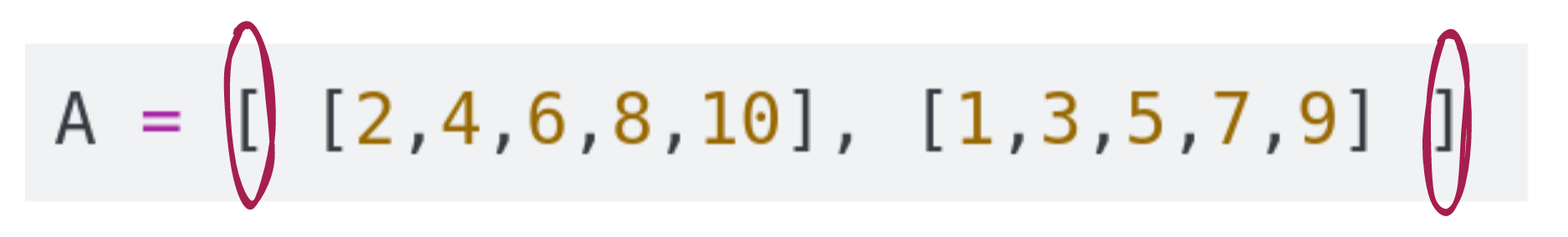
total = total + kAs it turns out, we can make a list of lists.
That is, a list whose elements are themselves lists.
For example:
A = [ [2,4,6,8,10], [1,3,5,7,9] ]

x = A[1]          # The 2nd element is a list
print(x)          # Prints [1,3,5,7,9]

y = A[1][3]       # 4-element of 2nd list
print(y)          # 7

print(len(A))     # 2
print(len(A[0]))  # 5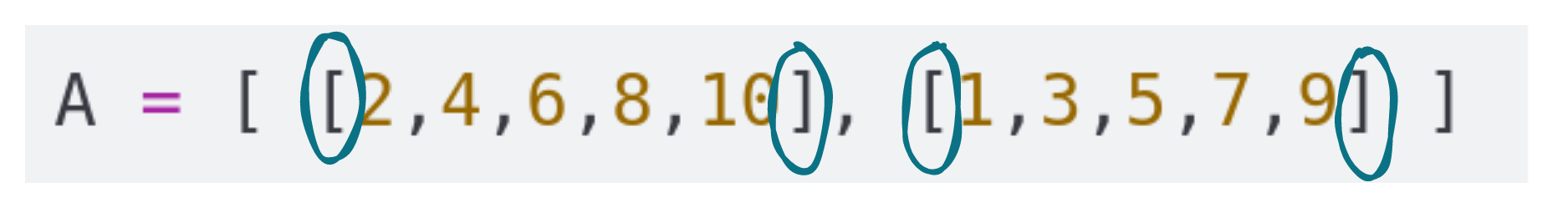
A[1] refers to the 2nd element of the outer list, which means A[1] is the 2nd inner listA[1] is a list itself, we can access its elements using an additional set of square brackets, e.g., A[1][3] = 7len() function applied to the whole list will give 2, while applying it to one of the constituent lists will give that list’s lengthThink of a single list as one dimensional:
A = [2, 4, 6, 8, 10]
print(A[3])
In a one-dimensional list, we need a single number to access a data value in the list: print(A [3])
A list of lists is two dimensional:
A = [ [2,4,6,8,10], [1,3,5,7,9] ]
print(A[0][2])
In a two-dimensional list, we need two numbers to access a data value in the list:, hence print(A[0][2])
Think of a list of lists of lists as three-dimensional, which means three numbers fix the position of a element. For example:
A = [ [ [1,2], [3,4], [5,6] ], [ [7,8], [9,10], [11,12] ] ]It’s a bit hard to see the list of lists of lists:

We can look at indexing list elements by looking at each element:
Get the outermost element:
A = [ [ [1,2], [3,4], [5,6] ], [ [7,8], [9,10], [11,12] ] ]

print(A[0])
[[1, 2], [3, 4], [5, 6]]Get the third element of the outermost element:
A = [ [ [1,2], [3,4], [5,6] ], [ [7,8], [9,10], [11,12] ] ]

print(A[0][2])
[5, 6]Get the second element of the third element of the outermost element:
A = [ [ [1,2], [3,4], [5,6] ], [ [7,8], [9,10], [11,12] ] ]

print(A[0][2][1])6Python was created as a general-purpose programming language and did not originally have support for numerical computing. A library called NumPy (numpy) was created to address this.
While lists are useful and easy to use, they are a bit inefficient “under the hood”:
Very large lists (million of elements or more) can slow down a program. A list-of-lists is even slower for large sizes, and takes up a lot of memory.
NumPy arrays (we will often call them simply “arrays”) were created as a separate structure in Python to enable efficient processing of lists of numbers, especially multidimensional lists.
Some of the most compelling uses involve the array equivalent of a list-of-lists-of-lists: an image. As we will see, a color image will can be represented as athree dimensional array while a black-and-white image only requires a two-dimensional array.
Because arrays are part of NumPy and not a “built-in” part of Python, the syntax around arrays is a bit different, for example:
import numpy as np

A = np.array([1,2,3,4])import numpy as np
A = np.array([1,2,3,4])
print(type(A)) # What does this print?
A[1] = 5 # Replace 2nd element
print(A) # [1 5 3 4]
print(A.shape[0]) # 4
print('len(A)=',len(A)) # 4
# A[4] = 9
# A.append(9)Let’s point out a few things: To gain efficiency, arrays trade away some flexibility and ease of use. For example, we now need to import this special package called numpy:
import numpy as npOnce we do this, the syntax for making an array with actual data is, as we’ve seen:
A = np.array([1,2,3,4])np ?
The convention to import the numpy library as np is strictly for convenience, using the keyword as to create a shortcut:
import numpy as np
A = np.array([1, 2, 3, 4])
This could also be written as:
import numpy
A = numpy.array([1,2,3,4])
There is no difference in the function of the code by creating the shorcut, but because we tend to use a lot of numpy arrays, the np shortcut saves time in writing code and makes the code more readable. It has become a convention in the Python/NumPy community, and you will rarely encounter import numpy without the np shortcut.
import numpy as np
A = np.array([1, 2, 3, 4])numpy``array function as a list:import numpy as np
A = np.array([1, 2, 3, 4]) # [1, 2, 3,4] is the argument for np.array() The actual array so created is assigned to the variable A. To work with elements in the array, we use square brackets with the variable A, just like a list:
A[1] = 5 # Replace 2nd elementThe standard function len() also works the same as with lists:
print('len(A)=',len(A))However, the array has a feature that is more general called shape:
print(A.shape[0]) # 4shape has.shape[0] has the first dimension (the length of the array along the first dimension).shape[1] has the length along the second dimension, and so on.shape[0].A = np.append(A, 9)
print(A) # [1 5 3 4 9]This creates a new array with the added element. The difference between what we have done here and modifying a list in place is subtle, but important. Typically most scientific applications do not change sizes on the fly, and so, this is not a serious restriction.
Numpy has powerful features that simplify manipulation of numeric arrays.
For example, consider:
Numpy also has a number of functions that act on arrays and return arrays, for example:
One can apply a function like square-root element-by-element:
A = np.array( [1, 4, 9, 16] )
B = np.sqrt(A)
print(B)        # [1. 2. 3. 4.]
Numpy can create an array with random elements, as in:
# Roll a die 20 times
A = np.random.randint(1, 7, size=20)
This produces an array of size 20 with each element randomly chosen from among the numbers 1,2,3,4,5,6.
Numpy has its own random-generation tool: np.random This has a function randint() that takes the desired range (inclusive of first, excluding the last), and the desired size of the array.
One can also test membership using the in operator: For example, suppose we roll a die 20 times and want to know whether a 6 occured:
# Roll a die 20 times
A = np.random.randint(1, 7, size=20)
if 6 in A:
print('Yes, there was a 6')Here, 2D is short for two-dimensional. Let’s begin with a conceptual depiction of a 1D (one-dimensional) array:
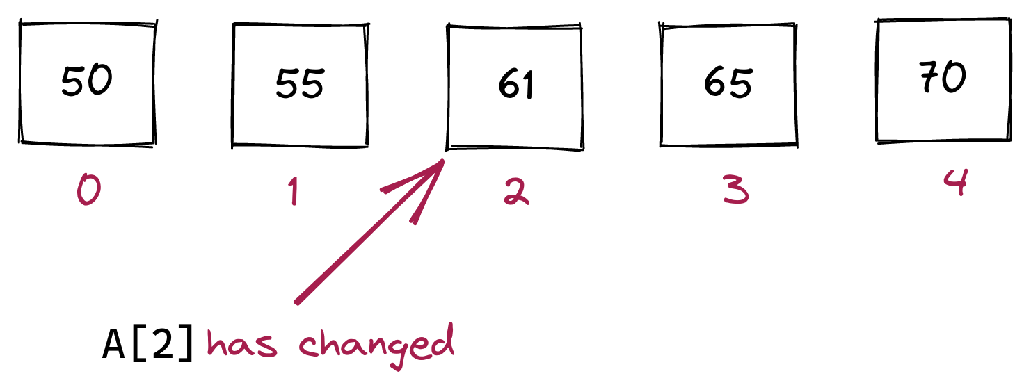
A = np.array([50, 55, 60, 65, 70])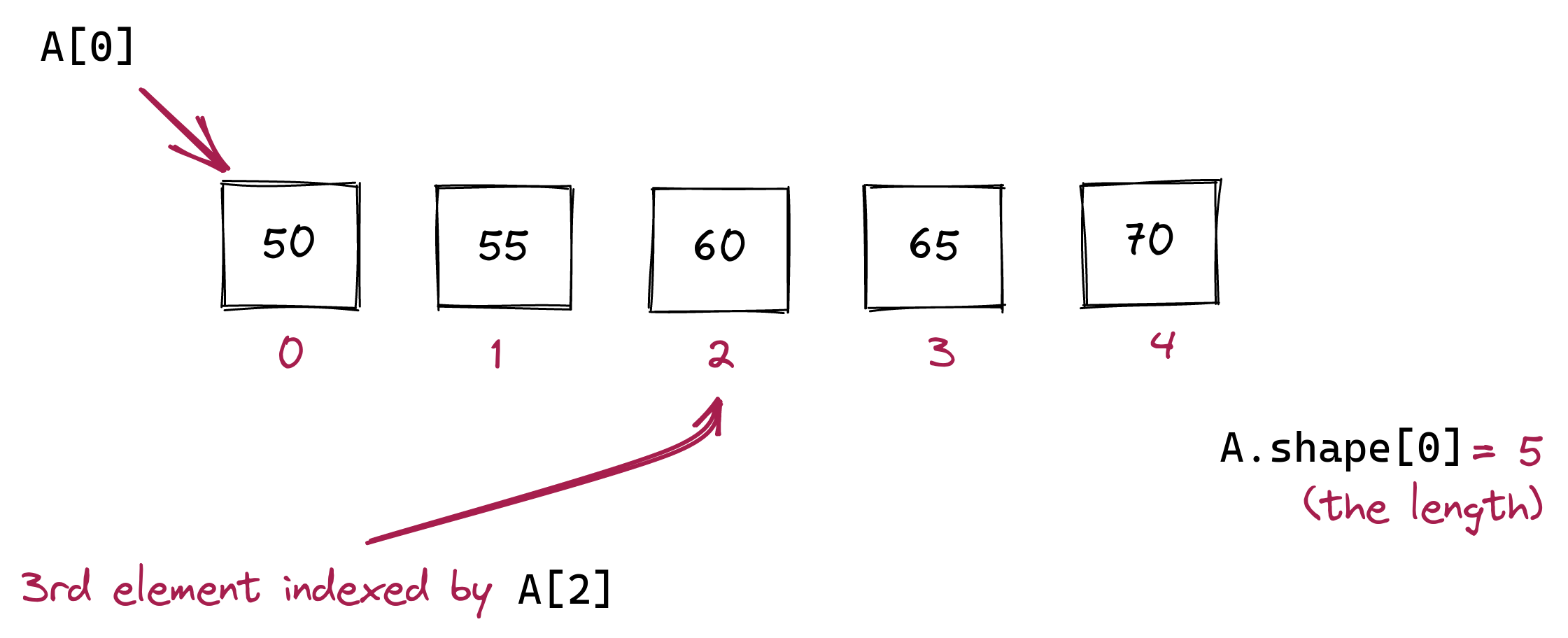
Because we need a way to use our keyboard to enter elements, we use a particular kind of syntax, comma-separation with square-brackets to specify the elements. We use a similar type of syntax to access a particular element in this array, as in:
print(A[2])We can also change an element in an array:
A[2] = 61which will result in the visualization:
To explain how a 2D array works, let’s start with its conceptual visualization, via an example:
Consider this visualization of a 2D array:
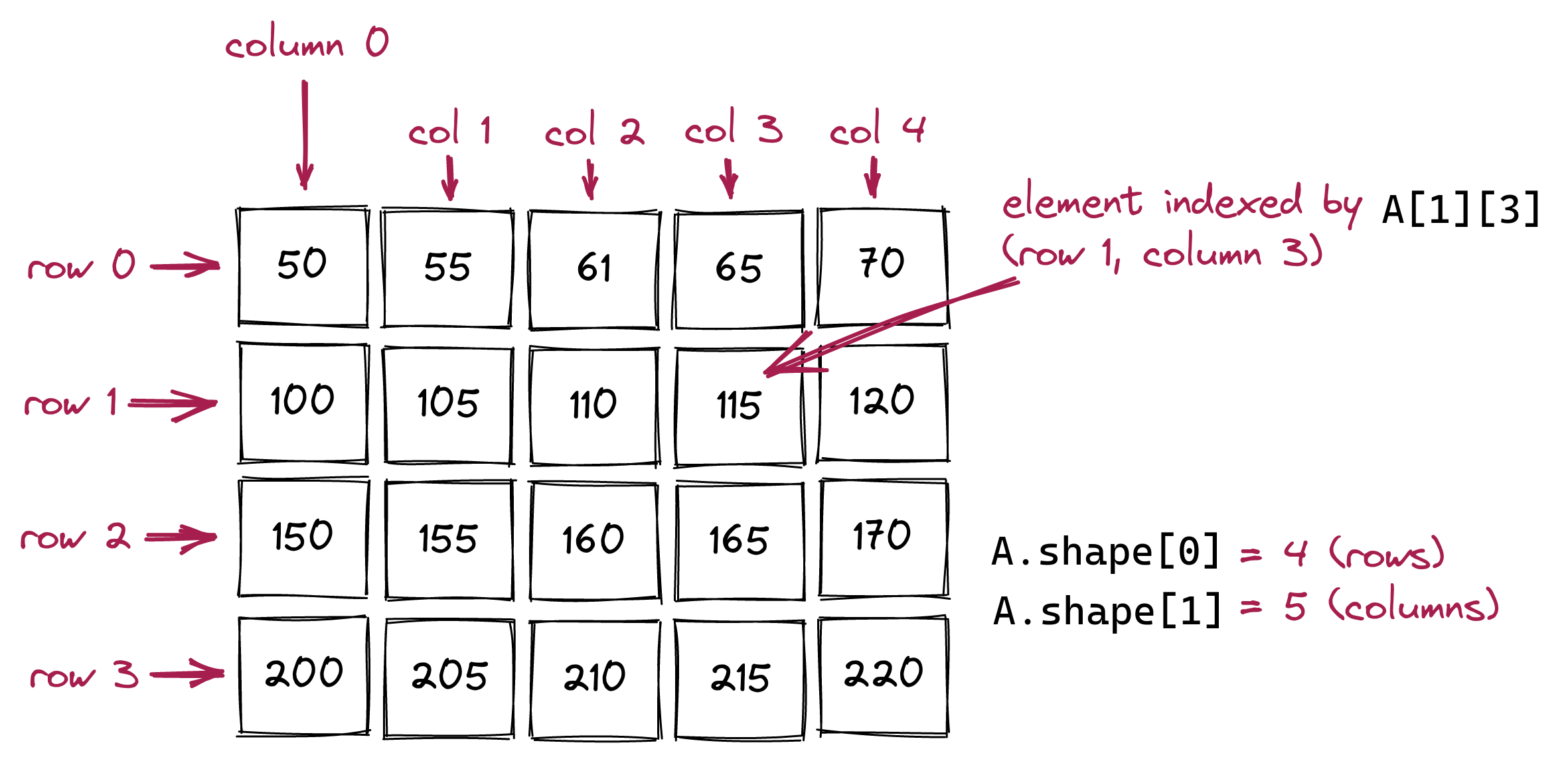
We use the term row to describe the contents going across one of the series of boxes going left to right:
And the term column (shortened to col in our pictures) to describe the series of boxes going vertically top to bottom:
A = np.array([ [50,   55,  60,  65,  70],
               [100, 105, 110, 120, 125],
               [150, 155, 160, 165, 170],
               [200, 205, 210, 215, 220] ])
Here, we’ve added whitespace (that’s allowed) to line up the rows so that it’s visually organized. To access a particular element, we need the row number and column number, as in:
print(A[1,3]) # NOT A[1][3]Important: Unlike a list-of-lists, arrays can use comma separation. For comparison:
# List of lists:
X = [ [2,4,6,8,10], [1,3,5,7,9] ]
print(X[0][2])

# 2D array:
X = np.array([ [2,4,6,8,10], [1,3,5,7,9] ])
print(X[0,2])
Arrays allow box separation as well (like lists) but this causes problems in other array operations (slicing): so please use comma-separation with a single set of square brackets for arrays.
Just as we used a for loop for a single array, it is very typical to use a nested for loop for a 2D array:
For comparison, let’s look at a 1D array:
A = np.array( [1, 4, 9, 16] )
for i in range(A.shape[0]):        # Recall: A.shape[0] is the size
    print(A[i])
The equivalent for a 2D array is:
A = np.array([ [50,   55,  60,  65,  70],
               [100, 105, 110, 120, 125],
               [150, 155, 160, 165, 170],
               [200, 205, 210, 215, 220] ])

for i in range(A.shape[0]):        # number of rows
    for j in range(A.shape[1]):    # number of columns
        print(A[i,j])
To make the code a bit more readable, we could write
num_rows = A.shape[0]
num_cols = A.shape[1]
for i in range(num_rows):
    for j in range(num_cols):
print(A[i,j])About 2D arrays:
Consider the following program:
from drawtool import DrawTool
import numpy as np

dt = DrawTool()
dt.set_XY_range(0,10, 0,10)
dt.set_aspect('equal')

greypixels = np.array([ [50,   55,  60,  65,  70],
                        [100, 105, 110, 120, 125],
                        [150, 155, 160, 165, 170],
                        [200, 205, 210, 215, 220] ])
dt.set_axes_off()
dt.draw_greyimage(greypixels)

dt.display()What is a greyscale image? By greyscale, we mean an image without colors, but rather shades of grey (often 256 shades). Consider this illustration showing an image on the left with a small part of it zoomed in:
![]()
Any digital image is really a 2D arrangement of small squares called pixels, in rows and columns (just like an array). In a greyscale image, each pixel is colored a shade of grey. In standard (“8-bit”) greyscale images, there are 256 shades of grey numbered 0 through 255, where 0 represents black and 255 represents white.
Now let’s go back to the code and examine what we wrote:
greypixels = np.array([ [50,   55,  60,  65,  70],
                        [100, 105, 110, 120, 125],
                        [150, 155, 160, 165, 170],
[200, 205, 210, 215, 220] ])Let’s now work with an actual image:
from drawtool import DrawTool
import numpy as np
dt = DrawTool()
dt.set_XY_range(0,10, 0,10)
dt.set_aspect('equal')
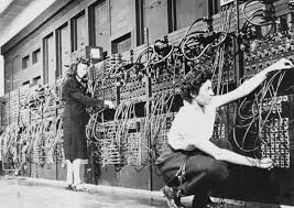
greypixels = dt.read_greyimagefile('eniac.jpg')
# greypixels is a 2D array
dt.set_axes_off()
dt.draw_greyimage(greypixels)
dt.display()
# Add code to print the number of rows, number of columns
# Should print: rows = 189 columns = 267Image formats:
.jpg in eniac.jpg) tells you the format.Let’s now modify a greyscale image:
from drawtool import DrawTool
import numpy as np

dt = DrawTool()
dt.set_XY_range(0,10, 0,10)
dt.set_aspect('equal')

greypixels = dt.read_greyimagefile('eniac.jpg')

greypixels2 = np.copy(greypixels)
num_rows = greypixels2.shape[0]
num_cols = greypixels2.shape[1]

lightness_factor = 10

for i in range(num_rows):
    for j in range(num_cols):
        value = greypixels[i,j] + lightness_factor
        if value > 255:
            value = 255
        greypixels2[i,j] = value

dt.set_axes_off()
dt.draw_greyimage(greypixels2)

# To save an image, use the save_greyimage() function:
# dt.save_greyimage(greypixels2,'eniac-light.jpg')

dt.display()In a color image, each pixel will have a color instead of a “greyness” value.
Unfortunately, one cannot easily represent colors with a single number.
There are many ways of using multiple numbers to encode colors.
We’ll use the most popular one: specify the strengths of the three primary colors (Red, Green, Blue).
This approach is so popular that we refer to it simply as “RGB.””
The “amount” of red is a number between 0 and 255, the amount of green is another such number, as is the amount of blue.
Each color is therefore a group of three numbers, for example:
(255,0,0) is all red (no green, no blue) (0,255,0) is all green (no red, no blue) (0,0,255) is all blue (no red, no green) Let’s try a few more:
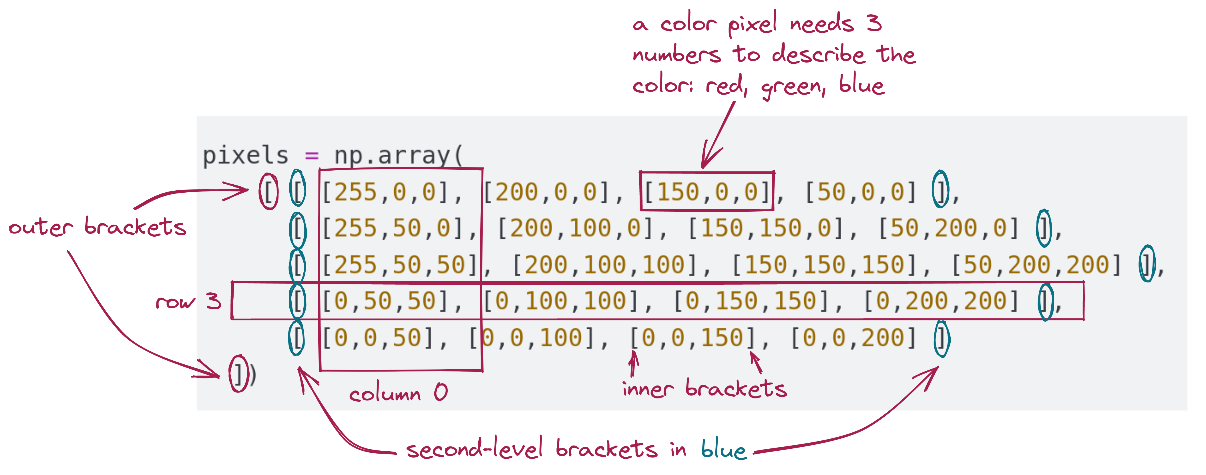
(255,255,0) (100,255,255) (200,200,200) (grey is R,G,B all equal) (0,0,0) (255,255,255) is white When each pixel needs three numbers and there’s a grid of pixels,how do we store the numbers?
Let’s look at an example:
from drawtool import DrawTool
import numpy as np

dt = DrawTool()
dt.set_XY_range(0,10, 0,10)
dt.set_aspect('equal')

pixels = np.array(
    [ [ [255,0,0], [200,0,0], [150,0,0], [50,0,0] ],
      [ [255,50,0], [200,100,0], [150,150,0], [50,200,0] ],
      [ [255,50,50], [200,100,100], [150,150,150], [50,200,200] ],
      [ [0,50,50], [0,100,100], [0,150,150], [0,200,200] ],
      [ [0,0,50], [0,0,100], [0,0,150], [0,0,200] ]
  ])

dt.set_axes_off()
dt.draw_image(pixels)

dt.display()
Let’s point out the structure inherent in the above 3D array:
Next, let’s work with actual color images with an example application: converting color to greyscale.
from drawtool import DrawTool
import numpy as np

dt = DrawTool()
dt.set_XY_range(0,10, 0,10)
dt.set_aspect('equal')

# The image file is expected to be in the same folder
pixels = dt.read_imagefile('washdc.jpg')

num_rows = pixels.shape[0]
num_cols = pixels.shape[1]

greypixels = dt.make_greypixel_array(num_rows, num_cols)
for i in range(num_rows):
    for j in range(num_cols):
        # Average of red/green/blue
        avg_rgb = (pixels[i,j,0] + pixels[i,j,1] + pixels[i,j,2]) / 3
        # Convert to int
        value = int(avg_rgb)
        greypixels[i,j] = value

dt.set_axes_off()
dt.draw_greyimage(greypixels)

# Notice: saving to a different image format (PNG):
dt.save_greyimage(greypixels, 'washdc-grey.png')

dt.display()Next, consider the following program:
from drawtool import DrawTool
import numpy as np

dt = DrawTool()
dt.set_XY_range(0,10, 0,10)
dt.set_aspect('equal')

pixels = dt.read_imagefile('washdc.jpg')

num_rows = pixels.shape[0]
num_cols = pixels.shape[1]

for i in range(num_rows):
    for j in range(num_cols):
        if ( (pixels[i,j,1] > pixels[i,j,0])
             and (pixels[i,j,2] < 0.5*pixels[i,j,1]) ):
            pixels[i,j,0] = 0
            pixels[i,j,1] = 0
            pixels[i,j,2] = 255

dt.set_axes_off()
dt.draw_image(pixels)

dt.display()What did we just do?
Slicing can be applied to arrays in the same way that we used them earlier for lists with one major difference, as we’ll point out. For example:
import numpy as np

print('list slicing')
A = [1, 4, 9, 16, 25, 36]
B = A[1:3]                 # B has [4, 9]
print(B)
B[0] = 5                   # B now has [5, 9]
print(B)
print(A)                   # What does this print?

print('array slicing')
A = np.array( [1, 4, 9, 16, 25, 36] )
B = A[1:3]                 # B "sees" [4, 9]
print(B)
B[0] = 5                   # What happens now?
print(B)
print(A) # What does this print?The slicing expression 1:3 in A[1:3] refers to all the elements from position 1 (inclusive) to just before position 3 (so, not including position 3). With lists, a new list is created with these elements:
A = [1, 4, 9, 16, 25, 36]
B = A[1:3]A = np.array( [1, 4, 9, 16, 25, 36] )
B = A[1:3] Here, array B refers to the segment (that’s still in A) from positions 2 to 3. This is why, if you make a change to B, you are actually changing A. Why did the authors of NumPy do this?
Slicing is a big sub-topic so we will point out a few useful things via an example:
# Color image:
A = np.array(
[ [ [255,0,0], [200,0,0], [150,0,0], [50,0,0] ],
[ [255,50,0], [200,100,0], [150,150,0], [50,200,0] ],
[ [255,50,50], [200,100,100], [150,150,150], [50,200,200] ],
[ [0,50,50], [0,100,100], [0,150,150], [0,200,200] ],
[ [0,0,50], [0,0,100], [0,0,150], [0,0,200] ]
])
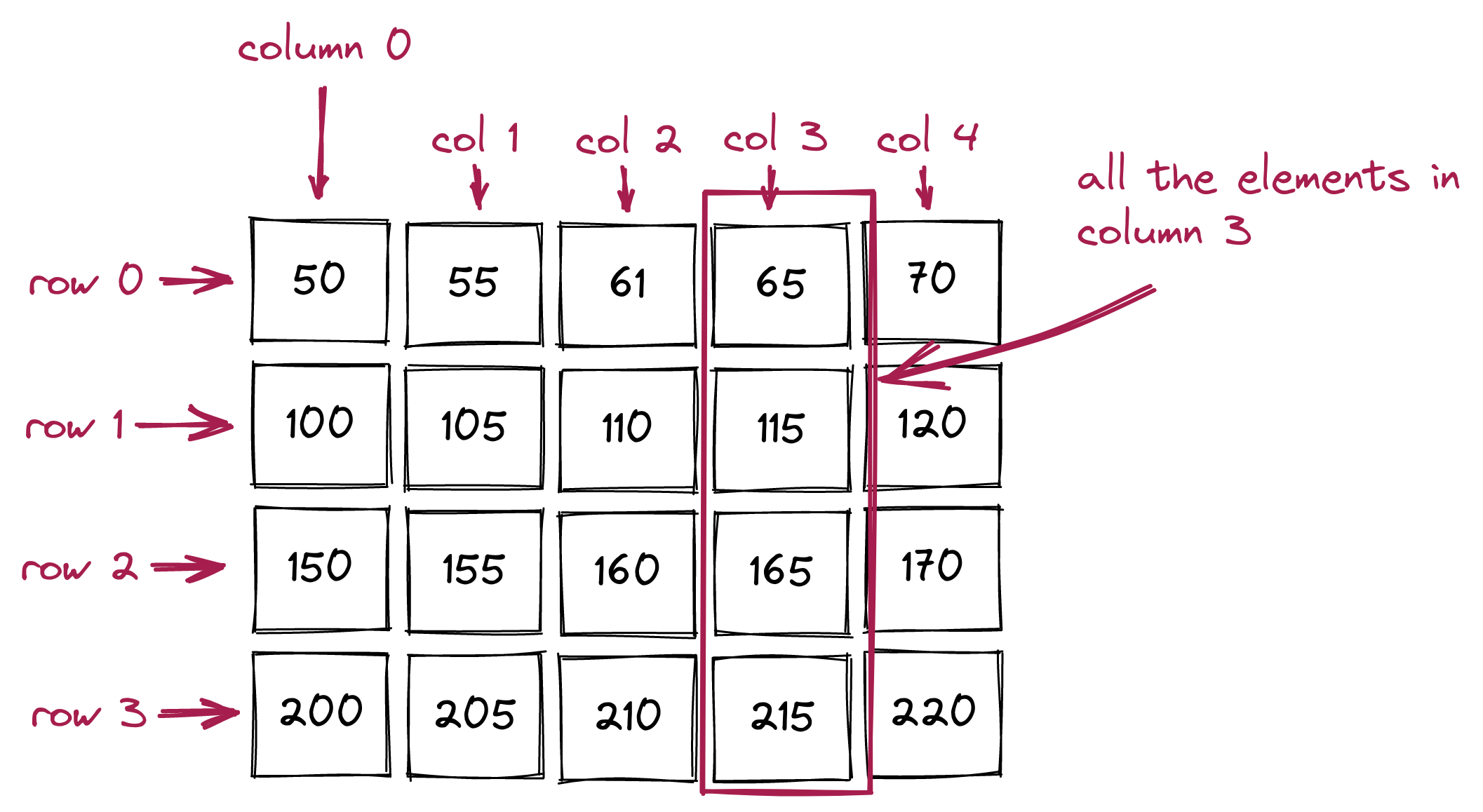
B = A[4:5,:,: ] # The fifth row
print(B)
C = A[:,1:2,:] # The second column
print(C)
D = A[:3,:2,:] # The pixels in the first three rows and first two columns
print(D)B = A[4:5,:,:]D = A[:3,:2,:]Let’s apply slicing to creating a cropped image:
Suppose we want to write a function that computes both the square and cube of a number. One option is to write two separate functions:
def square(x):
    return x*x

def cube(x):
    return x*x*x

x = 5
print(x, square(x), cube(x))
We can alternatively write one function that computes and returns two things:
def square_cube(x):
    square = x*x
    cube = square*x
    return (square, cube)

x = 5
(y, z) = square_cube(x)
print(x, y, z)return (square, cube).(y, z) = square_cube(x)We can go beyond a pair to any number of such “grouped” variables:
def powers(x):
    square = x*x
    cube = square*x
    fourth = cube*x
    fifth = fourth*x
    return (square, cube, fourth, fifth)  # returns four grouped variables

x = 5
(a, b, c, d) = powers(x) # expects four grouped variables from the function
print(x, a, b, c, d)
Such a grouping of variables is called a tuple.
Tuples are similar to lists in many ways, but different in one crucial aspect: tuples are immutable.
First, let’s examine how to write the same square_cube() function above but using lists:
def square_cube_list(x):
    square = x*x
    cube = square*x
    return [square, cube]

x = 5
[y, z] = square_cube_list(x)
print(x, y, z)
This works just fine. Another way in which a tuple is like a list is in using square-brackets and position indices to access individual elements, as in:
# List version:
L = square_cube_list(x)
print(L[0], L[1])      # L[0] has the square, L[1] has the cube

# Tuple version:
t = square_cube(x)
print(t[0], t[1])      # t[0] has the square, t[1] has the cube
However, here’s the difference:
# List version:
L = square_cube_list(x)
L[0] = 0              # This is allowed

# Tuple version:
t = square_cube(x)
t[0] = 0              # This is NOT allowed
Thus, you can replace a list element but you cannot replace a tuple element. This is in fact a bit subtle, as this example shows:
x = 3
y = 4
t = (x, y)   # The tuple's value is now fixed.
print(t)     # (3, 4)
x = 2
print(t)     # (3, 4)
Once the tuple is instantiated (that’s the technical term for “made”) then the tuple’s value cannot be changed. You can of course assign a different tuple value to a tuple variable as in:
t = (1, 2)
print(t)
t = (3, 4)
print(t)
Here, we’re simply replacing one fixed-value tuple with another. Hence, tuples are immutable (so are strings).
Why use tuples at all? It’s to allow programmers to signal clearly that their tuples shouldn’t be changed. This turns out to be convenient for mathematical tuples (like points on a graph), which are similar.
Groups of tuples can be combined into lists and other data structures. It’s very useful in working with points (the mathematical point you draw with coordinates) and other mathematical structures that need more than one number to describe.
For example, here’s a program that, given a list of points, finds the leftmost point (the one with the smallest x value).
def leftmost(L):
    leftmost_guess = L[0]
    for q in L:
        if q[0] < leftmost_guess[0]:
            leftmost_guess = q
    return leftmost_guess

list_of_points = [(3,4), (1,2), (3,2), (4,3), (5,6)]
(x,y) = leftmost(list_of_points)
print('leftmost:', (x,y) )
leftmost: (1, 2)Consider this problem: We have a data file that looks like this:
apple
banana
apple
pear
banana
banana
apple
kiwi
orange
orange
orange
kiwi
orange
This might represent, for example, a record of sales at a fruit stand. We’d like to count how many of each fruit. One way would be to define a counter for each kind:
num_apples = 0
num_bananas = 0
num_pears = 0
num_kiwis = 0
num_oranges = 0
with open('fruits.txt','r') as data_file:
    line = data_file.readline()
    while line != '':
        fruit = line.strip()
        if fruit == 'apple':
            num_apples += 1
        elif fruit == 'banana':
            num_bananas += 1
        elif fruit == 'pear':
            num_pears += 1
        elif fruit == 'kiwi':
            num_kiwis += 1
        elif fruit == 'orange':
            num_oranges += 1
        else:
            print('unknown fruit:', fruit)
        line = data_file.readline()

print('# apples:', num_apples)
print('# bananas:', num_bananas)
print('# pears:', num_pears)
print('# kiwi:', num_kiwis)
print('# oranges:', num_oranges)Aside from being tedious, this approach has other issues:
- One would like to be able to write a general program that does not need to know which fruits are in a file. - What if there were a thousand different kinds of items? - A single mistake in a variable can cause the counts to be wrong.
Fortunately, the use of dictionaries will make it easy:
# Make an empty dictionary
counters = dict()

with open('fruits.txt','r') as data_file:
    line = data_file.readline()
    while line != '':
        fruit = line.strip()
        if fruit in counters.keys():
            # If we've seen the fruit before, increment.
            counters[fruit] += 1
        else:
            # If this is the first time, set the counter to 1
            counters[fruit] = 1
        line = data_file.readline()

print(counters)d = {'apple': 3, 'banana': 3, 'pear': 1, 'kiwi': 2, 'orange': 4}In this case, we’re associating
d = {'apple': 3, 'banana': 3, 'pear': 1, 'kiwi': 2, 'orange': 4}

print(d['apple'])  # Prints 3

d['banana'] = 0
# Which changes the value associated with 'banana' to 3
The above is an example of a dictionary that’s already built (after we’ve processed the data). To process data on-the-fly, we need an additional operation that an English dictionary does not really have: we need to be able to add something that’s not already there. To add a new key, we simply use it as an index:
d = {'apple': 3, 'banana': 3, 'pear': 1, 'kiwi': 2, 'orange': 4}

d['plum'] = 0A dictionary can only have one value for each key. Assigning a second value to a key overwrites the original value.
d = {'apple': 3}
print(d)
d['apple'] = 4
print(d)
e = {'peach': 2, 'peach': 5}
print(e)
{'apple': 3}
{'apple': 4}
{'peach': 5}With this understanding we can now revisit the code in the fruit example.
# Make an empty dictionary
counters = dict()

with open('fruits.txt','r') as data_file:
    line = data_file.readline()
    while line != '':
        fruit = line.strip()
        if fruit in counters.keys():
            # If we've seen the fruit before, increment.
            counters[fruit] += 1
        else:
            # If this is the first time, set the counter to 1
            counters[fruit] = 1
        line = data_file.readline()

print(counters)if fruit in counters.keys(): checks to see if we have seen the fruit before by seeing if value of fruit is present as a key in the dictionary
counters[fruit] += 1 increments the count for that fruit by 1else statement), counters[fruit] = 1 adds a new key to the dictionary for that fruit, with value equal to 1 (since it has been seen for the first time)Unit 2 will lightly sketch a few advanced topics to introduce ideas and show some examples, without expecting mastery of all the details.
You might ask: what’s left in Python to learn?
Quite a lot. - Like many modern programming languages, Python is large enough that one needs a few courses to experience all of it. - Some concepts are advanced enough to need weeks to cover (example: objects). - Others need a background in data structures to understand how they work (example: dictionaries). - Yet others involve library functions and external packages.
Do you need to learn more? Is what you’ve learned enough to put Python to work? We’ll have more to say about this shortly.
Full credit is 100 pts. There is no extra credit.