Note 9: Searching & Sorting

This note is not really about searching and sorting, although we will certainly learn to search, and to sort.

This note is about computational complexity.

A Computational Experiment

Code

# imports
import numpy as np
import seaborn as sns
import pandas as pd

Let’s write a function to find the position (the index) of an integer within a list of integers:

def find_int(L:list, i:int) -> int | bool:
    for j in range(len(L)):
        if L[j] == i:
            return j
    return False

Using the interpreter, we can run it on a few examples and validate that it performs the functionality that we wish:

find_int([1, 3, 4, 5], 4)

find_int([1, 3, 4, 5], 7)

False

Let’s change the function now, to count the number of comparisons necessary to find the position of the integer:

def find_int(L:list, i:int) -> int:
    count = 0
    for j in range(len(L)):
        count += 1
        if L[j] == i:
            return count 
    return count

Now, we’ll run it on many inputs:

We will generate a list of sequential integers
We will pick a random element in the list to search for
We will search through the list to see how many comparisons were necessary to find the random element

num_comparisons = []
n_vals = []
for n in range(10,200):
    L = [1]
    for _ in range(n):
        L.append(L[-1] + np.random.randint(1,10))
    comparisons = []
    for _ in range(200):
        search_val = np.random.choice(L)
        comparisons.append(find_int(L, search_val))
    num_comparisons.append(np.mean(comparisons))
    n_vals.append(n)

Let’s plot the results, looking at how many comparisons were necessary, as compared to the length of the list:

sns.lineplot(x = n_vals, y = num_comparisons)

Plotting

Plotting in this note is accomplished using the seaborn library. You don’t need to know too many details about how seaborn works, but the documentation is very helpful, and it allows for much more expressive plotting than spreadsheet tools such as Microsoft Excel or Google Sheets.

The number of comparisons grows linearly with the number of elements in the list. If the number of elements in the list doubles, we expect the number of comparisons needed to double!

Can we do a better job searching through this list? Yes. How?

Let’s look at how our search progresses through a series of sorted integers. In the image below, our search function is looking for the integer 17.

The search iterates over each element of the list in sequence, until 17 is found.
- The red bar shows where the 17 is definitely not
- The green bar shows where the 17 might be
Each comparison eliminates one element from possibly being 17
- Except for the comparison that finds the 17
This search is called a sequential search or linear search

A more efficient search takes advantage of the fact that our list is sorted:

For any element in the list, if the element is less than 17, the 17 lies to the “right”
- If the element is greater than 17, the 17 lies to the left
If we start in the middle, we eliminate half of the remaining possible elements
- Each time through, we eliminate half of the remaining possible elements
- (Except for the comparison that finds the 17)

This search is called a binary search.

If we double the length of the list, we double the average number of comparisons required for linear search
If we double the length of the list, we increase the number of comparisons required for binary search by one comparison

This is an extremely important result. We can code and graph the results.

First, we’ll write a binary search:

def find_binary(L:list, i:int) -> int:
    count = 0
    left_end = 0
    right_end = len(L)
    while True:
        position = left_end + (right_end - left_end)//2
        if L[position] > i:
            count += 1
            right_end = position
        elif L[position] < i:
            count += 1
            left_end = position
        else:
            return count
    return count

Then, we’ll run the computational experiment using the binary search

num_comparisons_binary = []
n_vals = []
for n in range(10,200):
    L = [1]
    for _ in range(n):
        L.append(L[-1] + np.random.randint(1,10))
    comparisons = []
    for _ in range(200):
        search_val = np.random.choice(L)
        comparisons.append(find_binary(L, search_val))
    num_comparisons_binary.append(np.mean(comparisons))
    n_vals.append(n)

Finally, we’ll plot the results:

Code

df_plot = pd.DataFrame()
df_plot["Sequential"] = pd.Series(num_comparisons)
df_plot["Binary"] = pd.Series(num_comparisons_binary)
df_plot["N"] = pd.Series(n_vals)
df_plot["Comparisons"] = pd.Series(np.ones(len(n_vals)))
df_plot = pd.melt(df_plot, id_vars="N", value_vars=["Sequential", "Binary"], 
              var_name='Comparison Type', value_name="# Comparisons")
sns.lineplot(data=df_plot, x="N", y="# Comparisons", hue="Comparison Type")

We see as \(n\) (the size of the list) increases, the number of comparisons required for binary search grows much more slowly than the number of comparisons required for linear search.

Remember: binary search is faster on sorted lists. Not all lists are sorted, and sorting the list will take additional comparisons!

Analysis

We performed a computational experiment to examine the run times of the different searches, but we can examine the run times of these searches analytically.

The linear search is straightforward: assuming that the element we are searching for is equally likely to be at any position in the list, the average number of comparisons is the length of the list divided by two. We confirmed this result with our experiment.

The binary search is more complicated: doubling the length of the list increases the number of comparisons by one. Exponential growth in the length of the list results in linear growth in the number of comparisons: therefore, linear growth in the length of the list results in logarithmic growth in the number of comparisons:

With one item, the number of comparisons needed is 0
With two items, the number of comparisons needed is 1
With four items, the number of comparisons needed 2
With \(n = 2^k\) items, the number of comparisons needed is \(k\)
- \(k = \log_2n\)

Take care to remember that we are talking about the order of growth: the binary search actually has two comparisons per halving.

In these analysis, we use “big O” notation to describe the complexity of algorithm runtime:

Linear search is \(O(n)\)
Binary search is \(O(\log n)\)

This refers to the order of growth of the number of operations as the size of the problem grows. Big O notation is approximate, and in this case, refers to an average runtime for these algorithms. There are certain cases where linear search is faster than binary search: if the element we are looking for is the first element, linear search will find it with one comparison!

Sorting Basics

When searching for an item in a list, we compare items in the list to some fixed value (the search target).

When sorting a list, we compare items in the list to each other. This should give us an intuition that sorting a list will take longer than searching through a list (indeed, searching is a sub-task of sorting algorithms).

We’ll start looking at sorting with the bubble sort algorithm that you implemented earlier. The example below sorts a list in place.

def bubble_sort(L):
    sort_finished = False
    while not sort_finished:
        sort_finished = True
        for k in range(len(L)-1):
            if L[k] > L[k+1]:
                sort_finished = False
                temp = L[k]
                L[k] = L[k+1]
                L[k+1] = temp

How it works (sorting smallest to largest):

Iterate over sequential pairs of elements in the list
Compare: If any pair is “out of order” (first element is greater than second element)
- Swap: Swap the pair of elements

Illustrated:

The inefficiency of the algorithm is illuminated: swapping only moves any element in the list one position at a time. If the smallest element in the list starts as the last element, it must be swapped \(n-1\) times before it is in the correct position!

We can examine the runtime of the algorithm in terms of comparisons and swaps:

Each iteration through the list, \(n-1\) comparisons are performed
Each iteration through the list, some number of swaps are performed:
- If the list is sorted, \(0\) swaps are needed
- If the list is ‘perfectly’ unsorted (reverse order), \(n-1\) swaps are needed
- We can say that, on average, \(\frac{n}{2}\) swaps are needed
How many iterations through the list do we need?
- If the list is sorted, we need \(1\) iteration
- If the list is ‘perfectly’ unsorted, we need \(n\) iterations
- We can say that, on average, \(\frac{n}{2}\) iterations are needed are needed

How many comparisons do we need in total?

\(n-1\) comparisons each iteration
\(\frac{n}{2}\) iterations in total
\((n-1) \frac{n}{2}\) yields \(O(n^2)\) comparisons
- We remove constants and smaller terms for Big-O notation

How many swaps do we need in total?

\(\frac{n}{2}\) swaps each iteration
\(\frac{n}{2}\) iterations in total
\(\frac{n}{2} \frac{n}{2}\) yields \(O(n^2)\) swaps

We can plot how much faster \(O(n^2)\) grows than \(O(n)\) and \(O(\log n)\):

Code

n = 21
df_plot = pd.DataFrame()
df_plot["N"] = pd.Series(list(range(1,n)))
df_plot["Log"] = pd.Series([np.log(i) for i in range(1,n)])
df_plot["Linear"] = pd.Series(list(range(1,n)))
df_plot["Quadratic"] = pd.Series([i**2 for i in range(1,n)])

df_plot["Comparisons"] = pd.Series(np.ones(n-1))
df_plot = pd.melt(df_plot, id_vars="N", value_vars=["Log", "Linear", "Quadratic"], 
              var_name='Comparison Type', value_name="# Comparisons")
sns.lineplot(data=df_plot, x="N", y="# Comparisons", hue="Comparison Type")

Insertions and Swaps

Let’s consider a real use case for a sorted list: our list-based priority queue:

Before adding a new element, the priority queue is sorted by priority
When a new element is initially added to the queue:
- The queue is lengthened by one
- The queue is no longer sorted

A naïve implementation of this queue would append the new element, and then bubble sort the queue. You should not actually do this. Why not?

On average, the correct position for the new element could be any position
- \(\frac{n}{2}\) swaps are needed to move the new element to the correct position
- \(\frac{n}{2}\) iterations through the list are needed to accomplish these swaps
  - \(n\) comparisons are performed each iteration through the list
- The time complexity the insertion is \(O(n^2)\)

Contrast this with a simple insertion:

\(n\) comparisons are required to determine the correct insertion position
At most \(n/2\) swaps are needed to move the new element to the correct position
- We used list concatenation in our previous implementation, which is simple to program, but slow to run
- Concatenation requires creating a new list, which (invisible to us, in Python) copies portions of the original list
- Code up a swap-based implementation in the practice problems
Direct insertion is faster (linear time) than bubble sort (quadratic time)
- The fastest general-purposes sorts are \(O(n \log n)\)
- Direct insertion is always faster: it takes advantage of the fact that the queue, pre-addition of the new element, was already sorted

We Can Do Even Better

Priority queues are, in practice, implemented with a data structure known as a heap. The data structure is somewhat more complicated, but yields even better performance:

Average insertion time of \(O(1)\)
Worst-case insertion time of \(O(\log n)\)

We are deliberately working through different implementations of the priority queue to demonstrate how changes in algorithmic implementation of a solution can change runtime efficiency.

Insertion Sort

The insertion sort algorithm works off of this principle: it is straightforward to insert a single new element into a sorted list, resulting in a new sorted list. An unsorted list is used to build a sorted list in place by finding the correct position for the new element and swapping until the element is in position. A “sorted” and “unsorted” portion of the list are maintained, until the entire list is sorted.

def insertion_sort(L):
    for i in range(len(L)):
        print(L[i])
        j = i
        while L[j-1] > L[j] and j > 0:
            L[j-1], L[j] = L[j], L[j-1]
            j -= 1

The for loop visits each element in the original list (left to right)
The while loop the compares and swaps this element to right-to-left
- The left side of the list is already sorted
- The element is swapped to the left until it is in position

Insertion sort visits \(n\) elements (the outer for loop)
For each of these, on average, \(\frac{n}{2}\) comparisons and swaps are made
The result is \(O(n^2)\) comparisons and \(O(n^2)\) swaps

If, however, the initial list is sorted (or “close” to being sorted), performance is much nearer \(n\) comparisons and \(n\) swaps.

Merging Lists

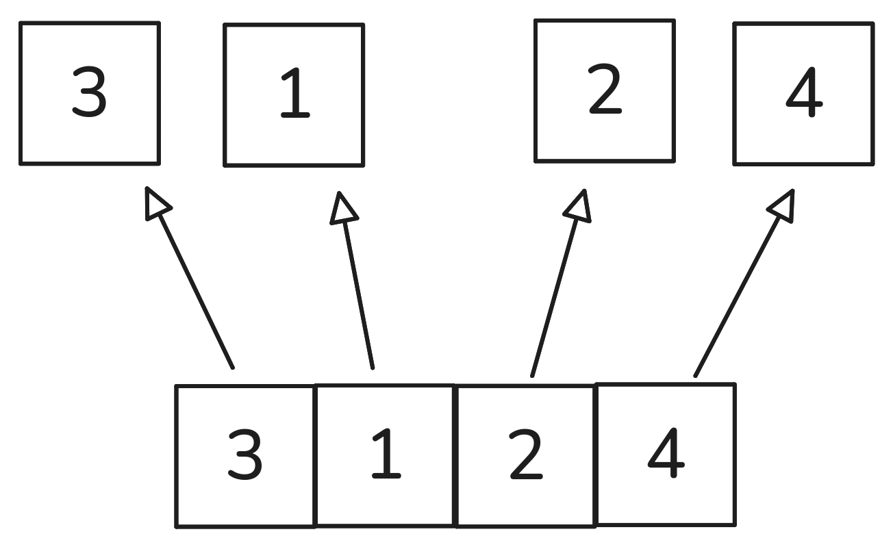
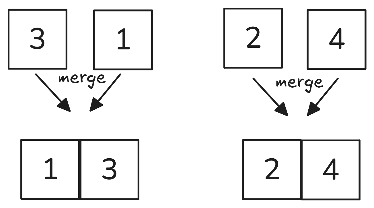
The basic “building block” of the more efficient merge sort algorithm is a function to merge two sorted lists into a new sorted list.

“Merge” runs in two parts:

First, while there are elements left in both input lists:
- Compare the first element of each input list
- Whichever is lower is removed from its input list and appended to the output list
- Loop until one input list is emptied
Once there are elements left in only one input list:
- Append the remaining elements of that input list to the output list, in order

Visualized:

In Python:

def merge_lists(L1, L2):
    L3 = []
    while len(L1) > 0 and len(L2) > 0:
        if L1[0] < L2[0]:
            L3.append(L1[0])
            L1 = L1[1:]
        else:
            L3.append(L2[0])
            L2 = L2[1:]
    while len(L1) > 0:
        L3.append(L1[0])
        L1 = L1[1:]   
    while len(L2) > 0:
        L3.append(L2[0])
        L2 = L2[1:]
    return L3

How many comparisons did it take to merge the two lists? The number of elements in the two lists, combined.

Merge Sort

Now that we can efficiently merge two lists, we can run the merge sort algorithm.

Start by breaking the input list up into individual elements
- Each element will be considered a “sub list” of length 1

These sub-lists are merged into larger sub-lists

These new sub-lists are merged into new sub-lists until the result is a single list

The average sub-list size doubles each merge step.

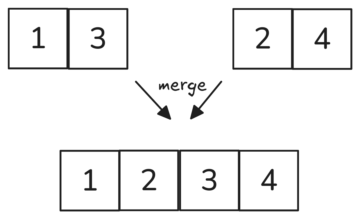
In Python:

def merge_sort(L):
    sub_lists = []    
    for l in L:
        sub_lists.append([l])
    
    new_sub_lists = []
    while len(new_sub_lists) != 1:
        new_sub_lists = []
        i = 0
        while i < len(sub_lists)-1:
            new_sub_lists.append(merge_lists(sub_lists[i], sub_lists[i+1]))
            i += 2
        if i == len(sub_lists)-1: #account for odd number of sub-lists
            new_sub_lists.append(sub_lists[-1])
        sub_lists = new_sub_lists
    
    return new_sub_lists[0]

Let’s look at the complexity of the sort for an input list of length \(n\):

Each merging step, a total of \(n\) elements are compared
Each merging step reduces the number of lists by half
- We’ve seen before that successive halving results in \(O(\log n)\)
The total average runtime of merge sort is \(O(n\log n)\)

Code

n = 21
df_plot = pd.DataFrame()
df_plot["N"] = pd.Series(list(range(1,n)))
df_plot["Log"] = pd.Series([np.log(i) for i in range(1,n)])
df_plot["Linear"] = pd.Series(list(range(1,n)))
df_plot["Loglinear"] = pd.Series([i*np.log(n) for i in range(1,n)])
df_plot["Quadratic"] = pd.Series([i**2 for i in range(1,n)])


df_plot["Comparisons"] = pd.Series(np.ones(n-1))
df_plot = pd.melt(df_plot, id_vars="N", value_vars=["Log", "Linear", "Loglinear", "Quadratic"], 
              var_name='Comparison Type', value_name="# Comparisons")
sns.lineplot(data=df_plot, x="N", y="# Comparisons", hue="Comparison Type")

Practice

Practice Problem 9.1

Implement a basic priority queue (using a list as the underlying data structure), and accomplish insertion using swaps rather than concatenation.

Practice Problem 9.2

Using two different implementations of a priority queue, one based on a list and one based on a linked list:

Write methods to insert new elements for both
Use Python’s random module to generate very large priority queues
- Measure the difference in runtime when inserting new elements into these enormous queues