r.5 Matrix-matrix multiplication and what it means
Multiplying one matrix by another produces a matrix, but
why is that and what good is it?
There are generally four contexts where we see matrix-matrix multiplication:
- Context #1.
When the matrices represent vector-transformations and they
multiply to create one matrix that does the combined transformation.
- Context #2.
When the associative rule is used to simplify terms.
- Context #3.
When a matrix's inverse multiplies into it to produce \({\bf I}\)
- Context #4.
When one matrix transforms another matrix (which is useful in
understanding row operations).
Before proceeding, let's address multiply-compatibility for
matrix-matrix and matrix-vector multiplication:
- Two matrices \({\bf A}_{m\times n}\) and \({\bf B}_{n\times k}\)
can be multiplied as \({\bf AB}\) to produce \({\bf C}_{m\times k}\).
$$
{\bf A}_{m\times n} {\bf B}_{n\times k} \eql {\bf C}_{m\times k}
$$
-
Thus, \({\bf B}\) should have as many rows as \({\bf A}\) has columns.
- The same rule works for matrix-vector compatibility if
we treat a column vector of dimension \(n\) as having
\(n\) rows:
$$
{\bf A}_{m\times n} {\bf x}_{n\times 1} \eql {\bf b}_{m\times 1}
$$
Let's start with the first context:
- Suppose \({\bf A}\) is a matrix that rotates a vector by
\(60^\circ\), and \({\bf B}\) is a matrix that reflects a vector
about the origin.
- Applying \({\bf A}\) to \({\bf x}=(2,3)\) gives
$$\eqb{
{\bf Ax}
& \eql &
\mat{\cos(60) & -\sin(60)\\
\sin(60) & \cos(60)}
\vectwo{2}{3} \\
& \eql &
\mat{0.5 & -0.866\\
0.866 & 0.5}
\vectwo{2}{3} \\
& \eql &
\vectwo{-1.59}{3.23} \\
& \defn &
{\bf y}
}$$
Here, we've named the result \({\bf y}\).
The "equals with the triangle" means "which we're defining as".
- Now, let's apply \({\bf B}\) to \({\bf y}\):
$$\eqb{
{\bf By}
& \eql &
\mat{-1 & 0\\
0 & -1}
\vectwo{-1.59}{3.23}
& \eql &
\vectwo{1.59}{-3.23}
& \defn &
{\bf z}
}$$
- We can write both products as:
$$
{\bf z} \eql {\bf B} ({\bf Ax})
$$
What this means:
- First apply \({\bf A}\) to \({\bf x}\).
- This produces a vector (we called it \({\bf y}\)).
- Then apply \({\bf B}\) to \({\bf y}\).
- The obvious question is: is there a matrix \({\bf C}\)
that will achieve the same thing directly:
$$
{\bf z} \eql {\bf Cx}?
$$
- If there was one, it would be natural to say that
$$
{\bf C} \eql {\bf BA}
$$
because we'd write
$$\eqb{
{\bf z} & \eql & {\bf B} ({\bf Ax})\\
& \eql & ({\bf B} {\bf A}) {\bf x}\\
& \eql & {\bf C} {\bf x}\\
}$$
- In fact, this is how the details of matrix multiplication
came about. If matrix-multiplication were done some other way, we
would not have the above result.
- In the above example, it turns out that
$$
{\bf BA} \eql
\mat{-1 & 0\\
0 & -1}
\mat{0.5 & -0.866\\
0.866 & 0.5}
\eql
\mat{-0.5 & 0.866\\
-0.866 & -0.5}
$$
So
$$
{\bf Cx} \eql
\mat{-0.5 & 0.866\\
-0.866 & -0.5}
\vectwo{2}{3}
\eql
\vectwo{1.59}{-3.23}
$$
as expected.
When we work out the algebra, it turns out that there are
two useful ways of describing matrix-matrix multiplication:
- We will describe \({\bf BA}\).
- The standard way is:
$$
\mat{
b_{11} & b_{12} & \cdots & b_{1n} \\
b_{21} & b_{22} & \cdots & b_{2n} \\
\vdots & \vdots & & \vdots \\
b_{n1} & b_{n2} & \cdots & b_{nn}
}
\mat{
a_{11} & a_{12} & \cdots & a_{1n} \\
a_{21} & a_{22} & \cdots & a_{2n} \\
\vdots & \vdots & & \vdots \\
a_{n1} & a_{n2} & \cdots & a_{nn}
}
\eql
\mat{
c_{11} & c_{12} & \cdots & c_{1n} \\
c_{21} & c_{22} & \cdots & c_{2n} \\
\vdots & \vdots & & \vdots \\
c_{n1} & c_{n2} & \cdots & c_{nn}
}
$$
where
$$
c_{ij} \eql \sum_{k=1}^n b_{ik} a_{kj}
$$
(this is the element in row i, column j of \({\bf C}\).
- If we "unpack" the matrix \({\bf A}\) into its columns
\({\bf a}_1, {\bf a}_2, \ldots \) then
this is one useful way to describe it:
$$
{\bf B}
\mat{a_{11} & a_{12} & \cdots & a_{1n}\\
a_{21} & a_{22} & \cdots & a_{2n}\\
a_{31} & a_{32} & \cdots & a_{3n}\\
\vdots & \vdots & \vdots & \vdots\\
a_{n1} & a_{n2} & \cdots & a_{nn}
}
\eql
{\bf B}
\mat{ & & & \\
\vdots & \vdots & \vdots & \vdots\\
{\bf a}_1 & {\bf a}_2 & \cdots & {\bf a}_n\\
\vdots & \vdots & \vdots & \vdots\\
& & &
}
\eql
\mat{ & & & \\
\vdots & \vdots & \vdots & \vdots\\
{\bf B a}_1 & {\bf B a}_2 & \cdots & {\bf B a}_n\\
\vdots & \vdots & \vdots & \vdots\\
& & &
}
$$
Here, the k-th column of the resulting \({\bf C}\) matrix
is the vector \({\bf Ba}_k\) that results from
the matrix \({\bf B}\) multiplying vector \({\bf a}_k\).
Let's look at cases where the second context arose:
- Matrix multiplication turned out (happily) to be associative:
$$
{\bf A} ({\bf BC}) \eql ({\bf AB}) {\bf C}
$$
This associativity turns out to be extremely useful in establishing
later results.
- Matrix multiplication, unfortunately, is not commutative.
That is, in general \({\bf AB} \neq {\bf BA} \)
Next, let's say a few things about matrix inverses:
- The inverse of a matrix \({\bf A}\), if it exists, is a
matrix \({\bf A}^{-1}\) such that
$$
{\bf A}^{-1} {\bf A} \eql {\bf I}
$$
where \({\bf I}\) is the identity matrix
$$
\mat{1 & 0 & \cdots & 0\\
0 & 1 & \cdots & 0\\
\vdots & \vdots & \vdots & \vdots\\
0 & 0 & \cdots & 1}
$$
Thus, \({\bf I}\) has 1's on the diagonal and 0's everywhere else.
- Here are some things to remember about \({\bf A}^{-1}\)
- It is defined only for square matrices.
- It's also true that \({\bf A} {\bf A}^{-1} = {\bf I}\)
- \({\bf A}^{-1}\) exists only if it's full rank.
- We compute \({\bf A}^{-1}\) this way:
- Identify the row operations that reduce \({\bf A}\) to
its RREF.
- Apply the same row operations to \({\bf I}\). The
resulting matrix is \({\bf A}^{-1}\).
- Of course the RREF procedure can reveal that \({\bf A}\)
is not full-rank (fewer pivots than columns), in which case
\({\bf A}^{-1}\) doesn't exist.
- What do we do when \({\bf A}\) is not square, or if \({\bf
A}^{-1}\) does not exist (cannot be computed)?
- One way out is least-squares, when we typically have too many
equations (more rows than columns).
- In this case, \({\bf A}^T {\bf A}\) is square and likely to
have an inverse.
- Recall the least-squares solution:
$$
\hat{\bf x}
\eql
({\bf A}^T {\bf A})^{-1}
{\bf A}^T {\bf b}
$$
Here we need the inverse \(({\bf A}^T {\bf A})^{-1}\) to exist.
- When there are many more rows than columns
\({\bf A}_{m\times n}\) has a few column vectors with many dimensions.
The likelihood that these are independent will be high.
- A somewhat difficult proof showed that if
the columns of \({\bf A}\) are independent then
\(({\bf A}^T {\bf A})^{-1}\) does indeed exist.
- The implication is that least-squares is very likely to work.
Finally, let's look at the fourth context:
matrix-multiplication as a "matrix transformer"
- When we multiply one matrix by another we get a third:
$$
{\bf AB} \eql {\bf C}
$$
- We could interpret this the same way we provided the
alternative interpretation of matrix-vector multiplication:
$$
{\bf Ax} \eql {\bf y}
$$
That is: matrix \({\bf A}\) transforms vector \({\bf x}\) into
vector \({\bf y}\).
- Thus, we could interpret
$$
{\bf AB} \eql {\bf C}
$$
as: \({\bf A}\) transforms matrix \({\bf B}\) into matrix \({\bf C}\).
- Such an interpretation does turn out to be useful for
theoretical purposes, as we'll see when reasoning about RREFs.
- So, now let's review key ideas in constructing an RREF.
- Let's start with an example:
$$\eqb{
2x_1 & \miss & 3x_2 & \plss & 2x_3 & \eql 5\\
-2x_1 & \plss & x_2 & & & \eql -1\\
x_1 & \plss & x_2 & \miss & x_3 & \eql 0\\
}$$
- We perform row operations to change the coefficients of
variables.
- For example, to change the coefficient of \(x_1\) in the
first equation to 1, we divide the entire first equation by 2:
$$\eqb{
{\bf 1} x_1 & \miss & {\bf 1.5} x_2 & \plss & {\bf 1} x_3 & \eql {\bf 2.5}\\
-2x_1 & \plss & x_2 & & & \eql -1\\
x_1 & \plss & x_2 & \miss & x_3 & \eql 0\\
}$$
- Of course, since all the manipulations are about
coefficients, it's cleaner if we work just with them,
incorporating the right side as well in the augmented matrix.
- Our starting point is the initial augmented matrix and
the identity matrix side-by-side:
$$
\left[
\begin{array}{ccc|c}
2 & -3 & 2 & 5\\
-2 & 1 & 0 & -1\\
1 & 1 & -1 & 0
\end{array}
\right]
\;\;\;\;\;\;\;\;\;\;\;\;
\mat{1 & 0 & 0 \\
0 & 1 & 0 \\
0 & 0 & 1}
$$
- So, applying the divide-by-2 to the first row:
$$
\left[
\begin{array}{ccc|c}
{\bf 1} & {\bf -1.5} & {\bf 1} & {\bf 2.5}\\
-2 & 1 & 0 & -1\\
1 & 1 & -1 & 0
\end{array}
\right]
\;\;\;\;\;\;\;\;\;\;\;\;
\mat{{\bf 0.5} & 0 & 0 \\
0 & 1 & 0 \\
0 & 0 & 1}
$$
Here, we're applying the exact same operation to the identity
matrix as well (for reasons we'll see).
- Since we replaced the first row with the original divided by
2, we write this as: \({\bf r}_1 \leftarrow \frac{{\bf r}_1}{2}\).
There are three types of row operations:
- Scale: divide one row by a number (like we did above)
$$
{\bf r}_i \leftarrow \frac{{\bf r}_i}{\alpha}
$$
- Swap: swap two rows
$$\eqb{
{\bf\mbox{temp}} & \leftarrow &{\bf r}_i\\
{\bf r}_i & \leftarrow & {\bf r}_j\\
{\bf r}_j & \leftarrow & {\bf\mbox{temp}}
}$$
- Replace a row by adding a multiple of another row.
$$
{\bf r}_i \leftarrow {\bf r}_i + \alpha {\bf r}_j
$$
You could devise others but these are enough.
There is also an order in which we change
coefficients:
- Always start with row 1, column 1, trying to make that
element a pivot.
- When we're successful making an element into a pivot,
we change coefficients below the pivot to zero.
- The search for the next pivot moves to the next row, next column.
- A search may not be successful, in which case we move to
the next column (same row).
- After the final pivot we go back to the first one and start
the process of creating zeroes above each pivot.
Here's what we get after making zeroes below the first
pivot:
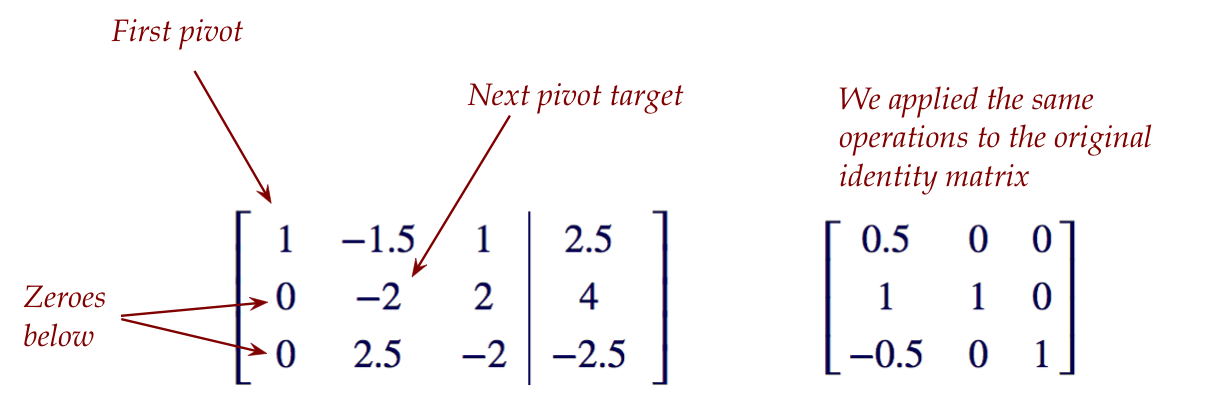
Continuing in this manner, we get the RREF (and by its side,
if the RREF is full-rank, the inverse):
$$
\left[
\begin{array}{ccc|c}
1 & 0 & 0 & 2\\
0 & 1 & 0 & 3\\
0 & 0 & 1 & 5
\end{array}
\right]
\;\;\;\;\;\;\;\;\;\;\;\;
\mat{-0.5 & 0.5 & 1 \\
1 & 2 & 2 \\
1.5 & 2.5 & 2}
$$
What we see:
- A full-rank RREF (a pivot in every column), which tells us
the equations have a unique solution.
- Notice: the non-augmented part of the full-rank RREF is the
identity matrix of that size.
- The solution itself is in the augmented column:
\(x_1=2, x_2=3, x_3=5\)
- We know this is the solution because we can convert back to
equations by looking at
$$
\left[
\begin{array}{ccc|c}
1 & 0 & 0 & 2\\
0 & 1 & 0 & 3\\
0 & 0 & 1 & 5
\end{array}
\right]
$$
- We get the inverse matrix on the right.
$$
{\bf A}^{-1} \eql
\mat{-0.5 & 0.5 & 1 \\
1 & 2 & 2 \\
1.5 & 2.5 & 2}
$$
So now let's turn to: why does this work?
- Clearly, manipulating the augmented matrix is the same thing
as manipulating the coefficients of the equations.
- So, if we end up with a full-rank RREF we know we just have
a different version of the same equations with the same solution
as the original.
- Seeing that the right-side matrix is the inverse needs some reasoning.
Consider the starting non-augmented matrix for the
equations example we've seen:
$$
{\bf A} \eql
\mat{
2 & -3 & 2 \\
-2 & 1 & 0 \\
1 & 1 & -1}
$$
- Define the matrix
$$
{\bf R}_1 \eql
\mat{0.5 & 0 & 0\\
0 & 1 & 0\\
0 & 0 & 1}
$$
- Left-multiply \({\bf A}\) by \({\bf R}_1\) :
$$
{\bf R}_1 {\bf A} \eql
\mat{0.5 & 0 & 0\\
0 & 1 & 0\\
0 & 0 & 1}
\mat{
2 & -3 & 2 \\
-2 & 1 & 0 \\
1 & 1 & -1}
\eql
\mat{
1 & -1.5 & 1 \\
-2 & 1 & 0 \\
1 & 1 & -1}
$$
- This shows that multiplication by \({\bf R}_1\)
achieves "multiply first row by 0.5" (or divide it by 2,
which is what we seek).
- In this way, \({\bf R}_1\) transforms \({\bf A}\) into
another matrix (making a pivot, which was our goal).
As we've seen all three types of row operations can be
achieved by a matrix multiplication that "transforms".
So, when we get an RREF at the end of \(k\) row operations
(transformations) we can describe it as:
$$
\mbox{RREF}({\bf A}) \eql
{\bf R}_k {\bf R}_{k-1} \ldots {\bf R}_2 {\bf R}_1 {\bf A}
$$
where the first row op is acheived by \({\bf R}_1\), the second
is represented by \({\bf R}_2\) applied to the result, and so on.
Recall: we applied these exact same transformations to the
identity matrix (in parallel, on the right side of our long list of
row ops).
- So, the question is: what do we get when applying
$$
{\bf R}_k {\bf R}_{k-1} \ldots {\bf R}_2 {\bf R}_1 {\bf I}
\eql ?
$$
- Let's go back to
$$
\mbox{RREF}({\bf A}) \eql
{\bf R}_k {\bf R}_{k-1} \ldots {\bf R}_2 {\bf R}_1 {\bf A}
$$
and do two things:
- Recognize that \( \mbox{RREF}({\bf A}) = {\bf I}\)
- Multiply all the \({\bf R}_i\) matrices into one matrix:
$$
{\bf R} \defn
{\bf R}_k {\bf R}_{k-1} \ldots {\bf R}_2 {\bf R}_1
$$
- Then, the reduction to RREF can be written as:
$$
{\bf I} \eql {\bf R} {\bf A}
$$
which means that \({\bf R}\) is the inverse of \({\bf A}\)!
Now, we don't actually maintain the products of row
operations for the sake of separately computing \({\bf R}\).
- Instead, we applied all the row ops to \({\bf I}\):
$$
{\bf R} {\bf I}
$$
- But this results in
$$
{\bf R} {\bf I} \eql {\bf R}
$$
So, the result at the end on the right side is the inverse
of \({\bf A}\) because \({\bf R}={\bf A}^{-1}\).
One last point: if we've already solved for the variables, why do we
need the inverse?
- Let's state this question as follows:
- We started with wanting to solve \({\bf Ax}={\bf b}\)
for some \({\bf A}\) and some \({\bf b}\), the given equations.
- We applied row reductions to get \(\mbox{RREF}({\bf A})\).
- That gave us the solution \({\bf x}\).
- Isn't that enough? Why also compute \({\bf A}^{-1}\) on
the right side?
- In applications, it turns out that very often the equations
stay the same but the right side changes to \({\bf Ax}={\bf c}\)
- In this case, we solve once to get \({\bf A}^{-1}\) and
apply it to a new right side:
$$
{\bf x} \eql {\bf A}^{-1} {\bf c}
$$
- In other applications like least-squares, we need
to compute the inverse of matrices like \(({\bf A}^T{\bf A})\).
- In fact, in general, linear algebra applications usually
care more about inverses than solving equations.
r.6 Spaces, span, independence, basis
Let's consider span first:
- We'll do this by example.
- Consider the 3D vectors
$$
{\bf u} \eql \vecthree{4}{0}{2}
\;\;\;\;\;\;\;\;
{\bf v} \eql \vecthree{0}{5}{3}
$$
- The span is all the vectors you can get by linear
combinations, which we formally write as:
$$
\mbox{span}({\bf u,v}) \eql \{{\bf z}: {\bf z} = \alpha{\bf u}
+ \beta{\bf v}, \mbox{ for some } \alpha,\beta\}
$$
How to read aloud: "all z such that z can be expressed as a linear
combination of u and v"
- These are 3D vectors, so what does the span look like?
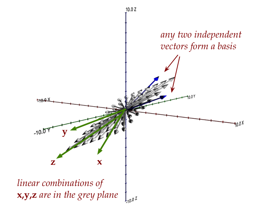
Let's draw some vectors in the span:
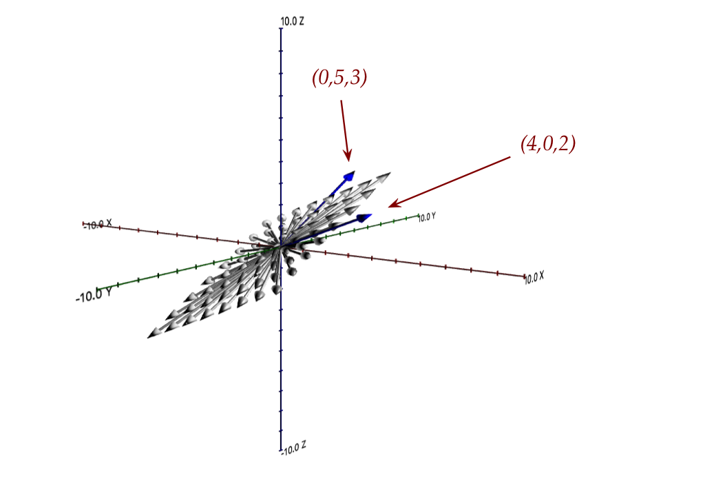
- All the vectors in the span lie in the plane containing
\({\bf u}\) and \({\bf v}\).
- The vector \((0,0,10)\), for example, which runs along the z-axis
is not in the span.
- Now look at the plane above and ask: is there any vector
in that plane that's not in \(\mbox{span}({\bf u,v})\)?
- No, because we can surely find a linear combination to reach it.
- Now for another important question: pick any three
vectors in that plane, and call them \({\bf x,y,z}\)
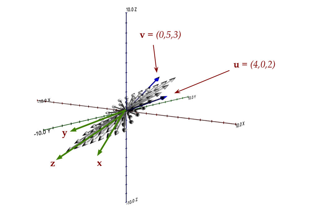
- Is every linear combination of these three
in the same plane?
- It seems obvious that the answer is yes because all
their parallelograms will lie in the plane.
- The implication is that the plane shown above is "complete"
in that it contains all linear combinations of any subset of
vectors.
- Such a collection is called a subspace.
- More formally: a subspace is a collection
of vectors where the linear combination of any two vectors is
in the collection.
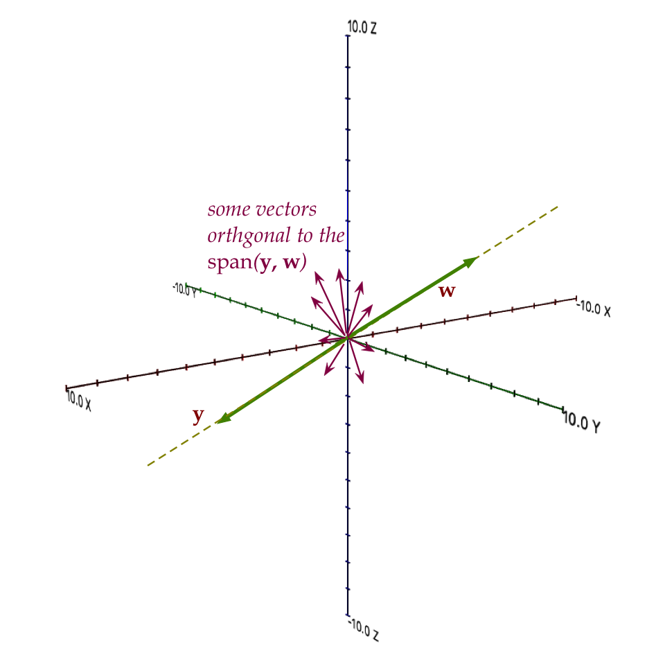
- Now consider the vectors \({\bf y}\) and \({\bf w}\) in this picture:
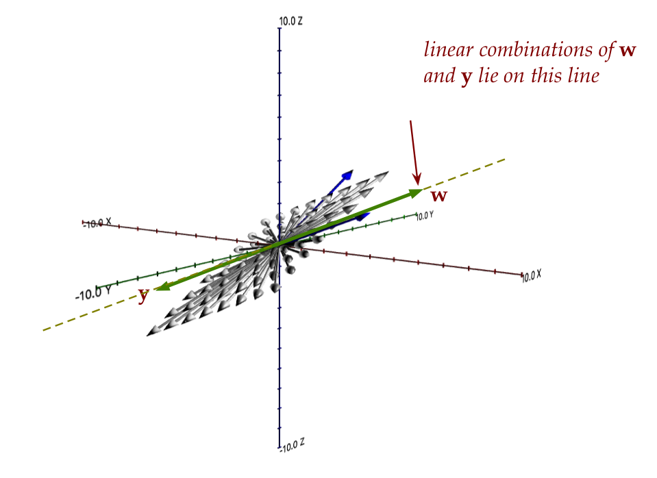
- Clearly all linear combinations of the two lie on the
dotted line, and so these two cannot
linearly generate every vector in the grey plane.
- The question we ask is: what is the minimum number of
vectors needed to span the grey plane?
- The answer is: two
- These could be any two non-collinear (independent!)
vectors like \({\bf u}\) and \({\bf v}\):
- We are led to the definition of a basis:
- A basis for a subspace is any minimal
collection of vectors whose span is the subspace.
- Observe: two vectors are not enough for all of 3D space.
- Could \({\bf u}\), \({\bf v}\) and \({\bf y}\) be a
basis for all of 3D space?
- A basis for 3D space needs three, and three that are not
co-planar (in the same plane).
- We are often interested in an orthogonal basis:
- Are \({\bf u}\) and \({\bf v}\) orthogonal?
- Let's check:
$$
{\bf u} \cdot {\bf v} \eql (4,0,2) \cdot (0,5,3) \eql 6 \neq 0
$$
So, no, they are not orthogonal and thus even though
\({\bf u}\) and \({\bf v}\) are a basis, they are not
an orthogonal basis.
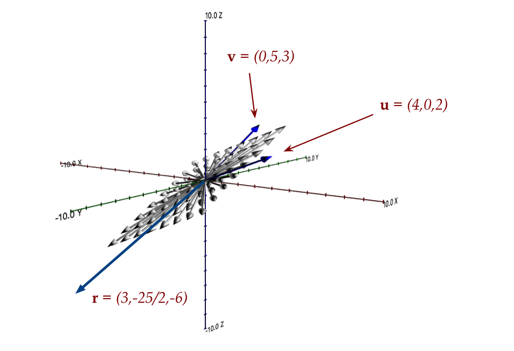
- Consider
\({\bf u}=(4,0,2)\) and \({\bf r}=(3,-\frac{25}{2}, -6))\)
$$
{\bf u} \cdot {\bf r} \eql (4,0,2) \cdot (3,-\frac{25}{2}, -6)
\eql 0
$$
So, these two are orthogonal and because two vectors are enough
for the grey plane, they form an orthogonal basis.
Orthogonal spaces:
- Let's go back to the vectors \({\bf y}\) and \({\bf w}\)
above, both of which were on the same line:
- Now, \(\mbox{span}({\bf y,w})\) is a subspace,
because all linear combinations of any two vectors on this
line are on the line.
- Consider all the vectors orthogonal to \({\bf y}\).
- These are all going to be on a plane to which the line
is perpendicular.
- Example vectors on this perpendicular plane are shown above.
- Let \({\bf S}\) be the subspace of vectors on this
perpendicular plane (perpendicular to the line).
- Notice: every vector in \({\bf S}\) is perpendicular
to every vector in \(\mbox{span}({\bf y,w})\).
- Thus, \({\bf S}\) and \(\mbox{span}({\bf y,w})\)
are orthogonal subspaces.
- There's notation for this:
$$
{\bf S}^\perp \eql \mbox{span}({\bf y,w})
$$
and
$$
{\bf S} \eql \mbox{span}({\bf y,w})^\perp
$$
- Orthogonal subspaces aren't really seen in practice, but
they are useful in proofs.
Let's review independence:
- Vectors \({\bf v}_1, {\bf v}_2, \ldots, {\bf v}_n\)
are linearly independent if the only
solution to the equation
$$
x_1 {\bf v}_1 + x_2 {\bf v}_2 + \ldots + x_n {\bf v}_n
\eql {\bf 0}
$$
is \(x_1 = x_2 = \ldots = x_n = 0\).
- Here, the \({\bf v}_i\)'s are vectors (any dimension: 2D,
3D, whatever).
- Every vector in the collection needs to be non-zero
(otherwise, trivially, a zero-vectors coefficient can be
anything, and the definition will fail).
- The \(x_i\)'s are numbers (scalars in the linear combination)
- Notice the right side: that's the zero vector of the same
dimension as any of the \({\bf v}_i\)'s
$$
{\bf 0} \eql (0,0,\ldots,0)
$$
- Consider these three vectors:
$$\eqb{
{\bf u} & \eql & (4,0,2) \\
{\bf v} & \eql & (0,5,3) \\
{\bf r} & \eql & (-3,-\frac{25}{2},-6) \\
}$$
Are they independent?
- Observe that
$$\eqb{
\frac{3}{4} {\bf u} - \frac{5}{2}{\bf v} - {\bf r}
& \eql &
\frac{3}{4}(4,0,2) - \frac{5}{2}(0,5,3) - (-3,-\frac{25}{2},-6)\\
& \eql & (0,0,0)
}$$
- So, in setting
$$
x_1 {\bf u} + x_2 {\bf u} + x_3 {\bf r} \eql {\bf 0}
$$
we know that \((x_1,x_2,x_3) = (\frac{3}{4}, -\frac{5}{2}, -1)\)
is one possible solution (there are others).
- This is a non-zero solution and hence the three are not
independent.
- Which makes sense since all three lie on the plane (from earlier):
- How can we check, given a collection of vectors, that they
are independent?
- Recall, we are asking for the solution to
$$
x_1 {\bf v}_1 + x_2 {\bf v}_2 + \ldots + x_n {\bf v}_n
\eql {\bf 0}
$$
- Place the vectors as columns of a matrix \({\bf A}\):
$$
{\bf A} \eql
\mat{
& & & \\
\vdots & \vdots & \ldots & \vdots \\
{\bf v}_1 & {\bf v}_2 & \ldots & {\bf v}_n\\
\vdots & \vdots & \ldots & \vdots \\
& & &
}
$$
- So,
$$
x_1 {\bf v}_1 + x_2 {\bf v}_2 + \ldots + x_n {\bf v}_n
\eql {\bf 0}
$$
becomes
$$
\mat{
& & & \\
\vdots & \vdots & \ldots & \vdots \\
{\bf v}_1 & {\bf v}_2 & \ldots & {\bf v}_n\\
\vdots & \vdots & \ldots & \vdots \\
& & &
}
\mat{x_1\\
x_2\\
x_3\\
\vdots\\
x_n}
\eql
\mat{0\\ 0\\ 0\\ \vdots\\ 0}
$$
- Or, more compactly: solve \({\bf Ax} = {\bf 0}\).
- This is something we know how to do (compute the RREF etc).
- From Theorem 8.1 we know that:
- When \(\mbox{RREF}({\bf A}) = {\bf I}\) (i.e., the RREF is
full-rank), then \({\bf x}={\bf 0}\) is the only solution to
\({\bf Ax} = {\bf 0}\).
- Thus, the vectors will be independent if the RREF is
full-rank (a pivot in every column).
- This gives us a means to identify whether a
collection of vectors is independent: put them in a matrix and
check its RREF.
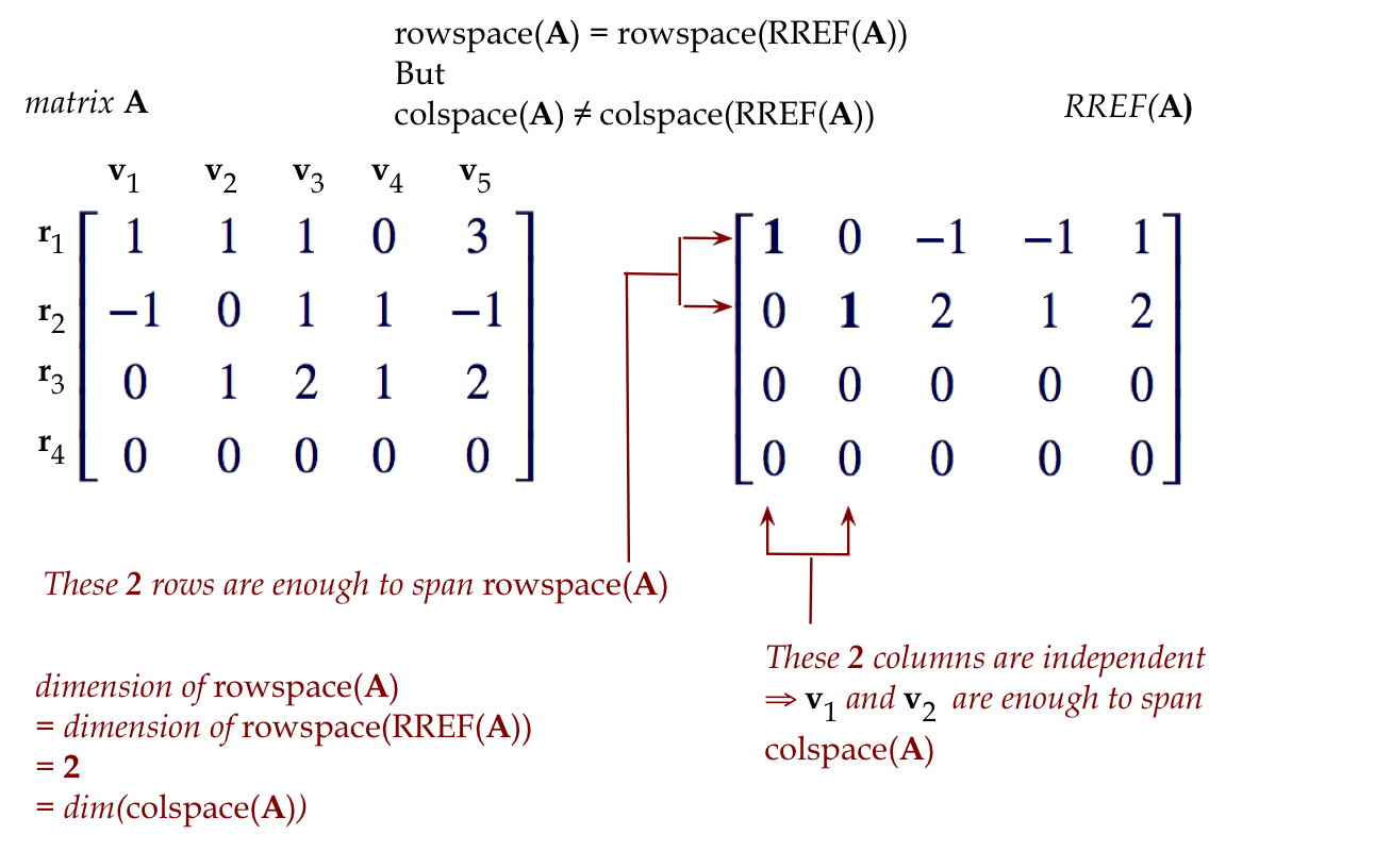
Lastly, let's review the rowspace and colspace of a matrix:
- Consider a matrix like
$$
{\bf A}
\eql
\mat{1 & 1 & 1 & 0 & 3\\
-1 & 0 & 1 & 1 & -1\\
0 & 1 & 2 & 1 & 2\\
0 & 0 & 0 & 0 & 0}
$$
- Let's treat the rows as vectors and name them:
$$\eqb{
{\bf r}_1 & \eql & (1,1,1,0,3)\\
{\bf r}_2 & \eql & (-1,0,1,1,-1)\\
{\bf r}_3 & \eql & (0,1,2,1,2)\\
{\bf r}_4 & \eql & (0,0,0,0,0)
}$$
- Then the span of these vectors is the rowspace of the matrix:
$$
\mbox{rowspace}({\bf A}) \eql \mbox{span}({\bf r}_1, {\bf r}_2,
{\bf r}_3, {\bf r}_4)
$$
- That is, any linear combination of the four row vectors is in
the rowspace.
- Example:
$$\eqb{
2{\bf r}_1 + 3 {\bf r}_2 + 0 {\bf r}_3 +5 {\bf r}_4
& \eql &
2(1,1,1,0,3) + 3(-1,0,1,1,-1) + 0(0,1,2,1,2) + 5(0,0,0,0,0)\\
& \eql &
(-1,2,5,3,3)
}$$
So \((-1,2,5,3,3)\) is a vector in the rowspace.
- Similarly, if we name the 5 columns \({\bf c}_1, {\bf c}_2,
{\bf c}_3,{\bf c}_4,{\bf c}_5\) then the colspace is their span:
$$
\mbox{colspace}({\bf A}) \eql \mbox{span}({\bf c}_1, {\bf c}_2,
{\bf c}_3,{\bf c}_4,{\bf c}_5)
$$
- What's of interest here is:
- What is the dimension of the
rowspace, that is, how many vectors are needed for a basis of the rowspace?
- (same question for colspace)
- Now the RREF turns out to be:
$$
\mat{{\bf 1} & 0 & -1 & -1 & 1\\
0 & {\bf 1} & 2 & 1 & 2\\
0 & 0 & 0 & 0 & 0\\
0 & 0 & 0 & 0 & 0}
$$
- Clearly, the rowspace of the RREF is the span of
the first two rows.
- Now for the key observation: the row operations we performed
do not change the rowspace of the matrices along the way from
\({\bf A}\) to its RREF.
- Why?
- All row operations are linear combinations of
rows.
- To see why, just recall how we wrote them. Example:
\({\bf r}_1 \leftarrow {\bf r}_1 - 2{\bf r}_2\).
- Unfortunately, it is not true that
\(\mbox{colspace}({\bf A}) = \mbox{colspace}(RREF({\bf A}))\).
- What is true is that the size of the basis for
\(\mbox{colspace}({\bf A})\)
is the same as the number of pivot columns.
- Because pivots are alone in both their rows and columns, we
get the remarkable result that the dimension of the rowspace
is the same as the dimension of the colspace.
- All of this is summarized in a picture we saw before:
r.7 Orthogonality
There are two subtopics of orthogonality that commonly appear in
applications:
- Orthogonal vectors and matrices.
- Projections.
Let's start with orthogonal vectors:
- Two vectors \({\bf u}\) and \({\bf v}\) are orthogonal if
$$
{\bf u} \cdot {\bf v} \eql 0
$$
Note:
- The right side is the number 0 (since the dot product
gives us a number).
- This is unlike the linear independence definition where the
\({\bf 0}\) on the right side is the zero vector.
- The definition comes from the angle between them, which
is a right-angle:
$$
\cos(\theta) \eql \frac{ {\bf u} \cdot {\bf v}}{ |{\bf u}||{\bf v}|}
$$
Since the lengths aren't zero, if the dot product is zero, that
implies a zero cosine, or \(\theta=90^\circ\).
- This definition extends to a collection of vectors:
- Consider vectors \({\bf v}_1,{\bf v}_2,{\bf v}_3\).
- The collection is orthogonal if
$$\eqb{
{\bf v}_1 \cdot {\bf v}_2 & \eql & 0\\
{\bf v}_1 \cdot {\bf v}_3 & \eql & 0\\
{\bf v}_2 \cdot {\bf v}_3 & \eql & 0
}$$
Since dot-product is commutative we don't need to specify
products like \({\bf v}_2 \cdot {\bf v}_2 = 0\).
- Example: \({\bf v}_1=(4,4,4), {\bf v}_2=(4,-8,4), {\bf v}_3=(6,0,-6)\)
$$\eqb{
{\bf v}_1 \cdot {\bf v}_2
& \eql & (4,4,4) \cdot (4,-8,4) & \eql & 0\\
{\bf v}_1 \cdot {\bf v}_3
& \eql & (4,4,4) \cdot (6,0,-6) & \eql & 0\\
{\bf v}_2 \cdot {\bf v}_3
& \eql & (4,-8,4) \cdot (6,0,-6) & \eql & 0\\
}$$
- Now consider this equation
$$
\alpha_1 {\bf v}_1 + \alpha_2 {\bf v}_2 + \alpha_3 {\bf v}_3
= {\bf 0}
$$
Does this imply that all the \(\alpha\)'s are zero, and therefore the
\({\bf v}\)'s are independent?
- Multiply (dot product) both sides by \({\bf v}_1\):
$$
{\bf v}_1 \cdot (\alpha_1 {\bf v}_1 + \alpha_2 {\bf v}_2 + \alpha_3 {\bf v}_3)
\eql {\bf v}_1 \cdot {\bf 0}
$$
- The right side becomes the number 0.
- Do the algebra on the left side, passing the dot into the parens:
$$
\alpha_1 ({\bf v}_1 \cdot {\bf v}_1) + \alpha_2 ({\bf v}_1 \cdot {\bf v}_2) + \alpha_3 ({\bf v}_1 \cdot {\bf v}_3)
\eql 0
$$
- Because they are orthogonal, only non-zero dot product is
the first one, so
$$
\alpha_1 ({\bf v}_1 \cdot {\bf v}_1) + 0 + 0
\eql 0
$$
- Now apply the dot product
$$
{\bf v}_1 \cdot {\bf v}_1 \eql |{\bf v}_1| |{\bf v}_1| \cos(0)
$$
- And so, we get
$$
\alpha_1 |{\bf v}_1| |{\bf v}_1|
\eql 0
$$
- Which, because \(|{\bf v}_1| \neq 0\), implies that
$$
\alpha_1 \eql 0
$$
- To conclude, an orthogonal collection is linearly
independent.
- This makes sense geometrically too.
- For example, with the three vectors in the example above:
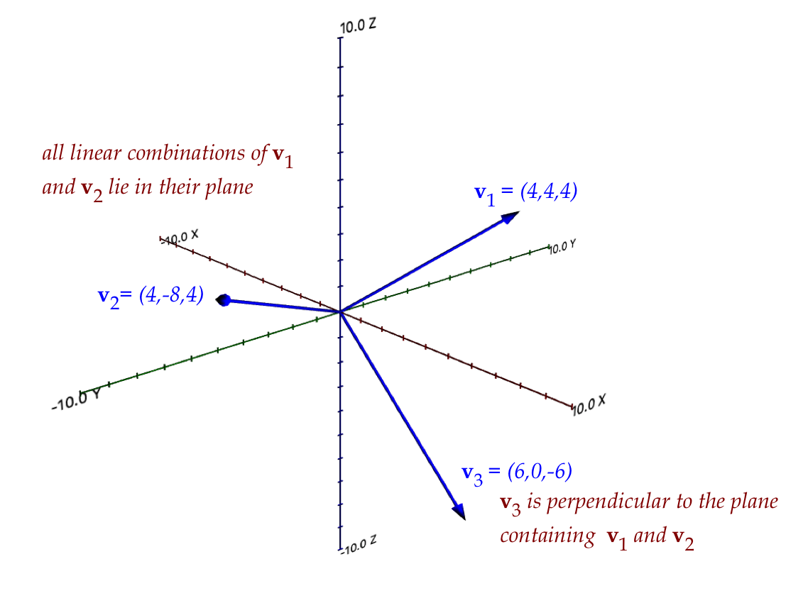
- \({\bf v}_3\) is not in the plane of
\({\bf v}_1\) and \({\bf v}_2\), and so, cannot
be expressed as a linear combination of \({\bf v}_1\) and \({\bf v}_2\).
What about complex vectors?
- The visualization problem with complex vectors (even 2D complex vectors) is
that we can't draw them.
- For example, consider these two 3-component complex vectors:
$$\eqb{
{\bf u} & \eql & (1 + 0i, \; -0.5 + 0.866i, \; -0.5 - 0.866i)\\
{\bf v} & \eql & (1 + 0i, \; 1 + 0i, \; 1 + 0i)
}$$
- We can't really visualize because there's no convenient way
of drawing a complex vector like this, and so, there's no geometric
way to define an angle between them.
- However, their dot-product is:
$$
(1 + 0i)(1 - 0i) + (-0.5+0.866i)(1-0i) + (-0.5 - 0.866i)(1 - 0i)
\eql 0
$$
(Recall: we conjugate the elements of the second vector.)
- Thus, we define orthogonality between two complex
vectors to mean: their dot-product is zero.
Orthogonal matrices
- First, let's sort out orthogonal vs orthonormal.
- Two vectors \({\bf u}\) and \({\bf v}\)
are orthonormal if
- They are orthogonal.
- They have unit length: \(|{\bf u}| = 1\), \(|{\bf v}| = 1\)
- There is, unfortunately, a bit of confusing nomenclature
regarding orthogonal matrices.
- An orthogonal matrix is a matrix whose columns are
pairwise orthonormal.
- Note: pairwise means "all possible pairs" like
column 2 and column 5.
- For example, consider
$$
{\bf A} \eql
\mat{4 & 4 & 6\\
4 & -8 & 0\\
4 & 4 & -6}
$$
You can check that the columns are pairwise orthogonal
but not orthonormal.
- For example: \(|(4,4,4)| = \sqrt{4^2+4^2+4^2} = 6.92820\).
- However, this matrix is orthonormal:
$$
{\bf Q} \eql
\mat{0.577 & 0.408 & 0.707\\
0.577 & -0.816 & 0.408\\
0.577 & 0 & -0.707}
$$
The columns are pairwise orthogonal and all have unit length.
- What's nice about an orthonormal matrix is this:
$$
{\bf Q}^T {\bf Q} \eql {\bf I}
$$
- With the above example:
$$
{\bf Q}^T {\bf Q} \eql
\mat{0.577 & 0.577 & 0.577\\
0.408 & -0.816 & 0\\
0.707 & 0.408 & -0.707}
\mat{0.577 & 0.408 & 0.707\\
0.577 & -0.816 & 0.408\\
0.577 & 0 & -0.707}
\eql
\mat{1 & 0 & 0\\
0 & 1 & 0\\
0 & 0 & 1}
$$
To see why:
- The row i, column j entry of the product is
the dot product of row i from \({\bf Q}^T\)
and column j from \({\bf Q}\)
- But row i from \({\bf Q}^T\) is just column i from \({\bf Q}\)
- When \(i\neq j\)
column i and column j from \({\bf Q}\) are orthonormal and
so their dot-product is 0.
- When i=j, it's the dot-product of a column with itself,
which is 1.
- The important implication is that \({\bf Q}^T\) is the
inverse of \({\bf Q}\).
r.8 Projections
Let's start with a 2D example:
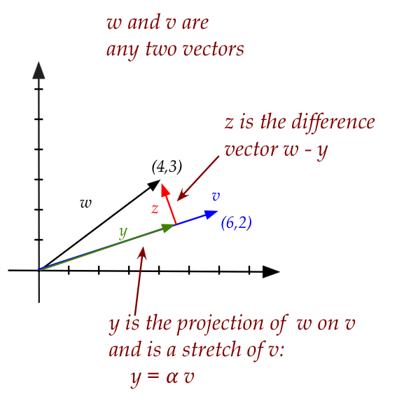
- Here, \({\bf w}\) and \({\bf v}\) are any two vectors.
- The projection of \({\bf w}\) on \({\bf v}\) is
that vector \({\bf y}\) along \({\bf v}\) which will make the difference
perpendicular (dot product zero):
$$
({\bf w} - \alpha{\bf v}) \cdot {\bf v} \eql 0\\
$$
That is, there is some stretch \(\alpha {\bf v}\) of
\({\bf v}\) which will make the difference \({\bf z}\) perpendicular
to \({\bf v}\).
- We can solve for the number \(\alpha\):
$$
\alpha \eql \frac{{\bf w} \cdot {\bf v}}{{\bf v} \cdot {\bf v}}
$$
- When, for example,
$$\eqb{
{\bf w} & \eql & (4,3) \\
{\bf v} & \eql & (6,2)
}$$
we get
$$
\alpha \eql \frac{(4,3) \cdot (6,2)}{(6,2) \cdot (6,2)}
\eql 0.75
$$
- Although we have drawn the above with 2D vectors, a
projection from one vector to another works in any number of
dimensions, for example:
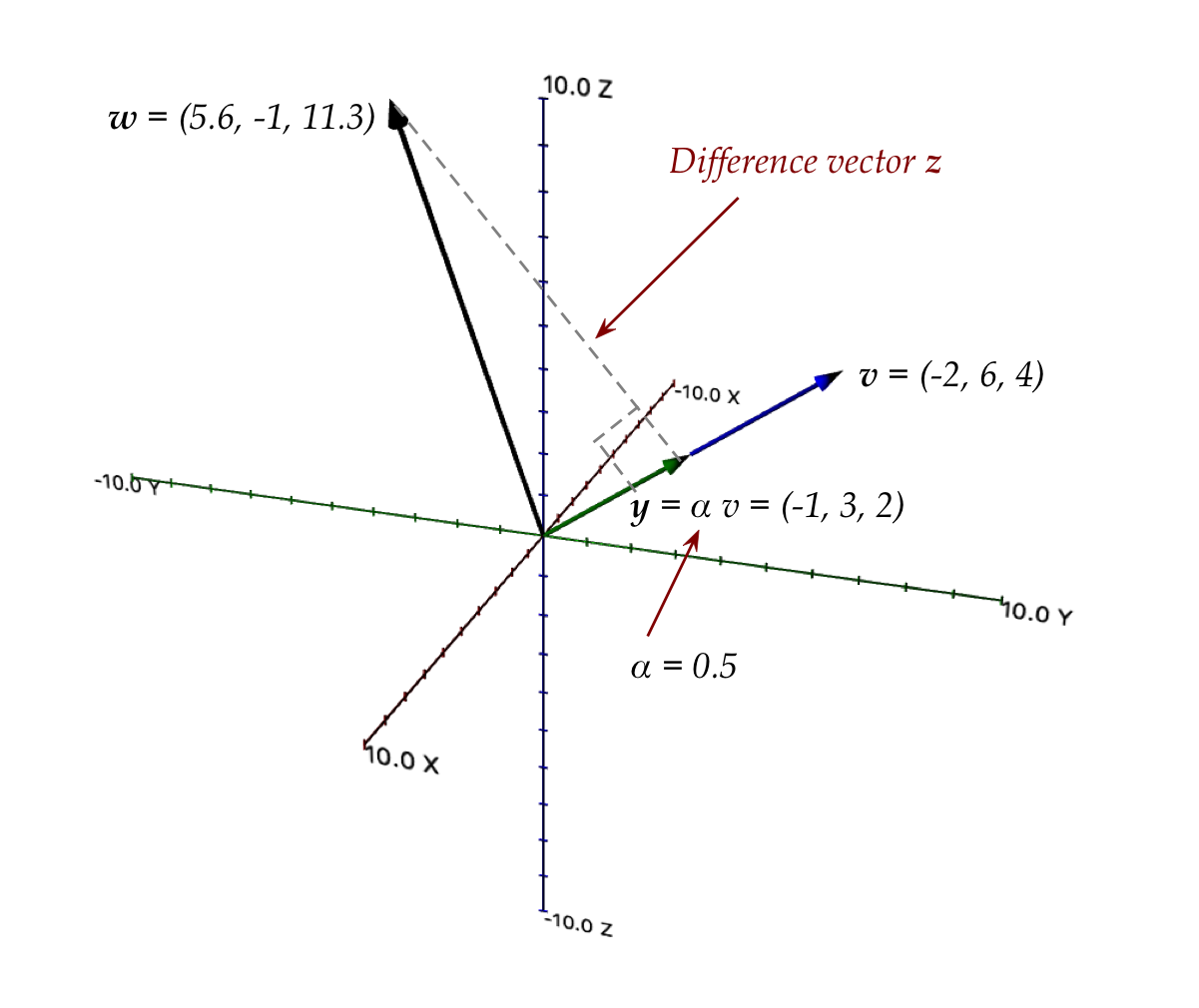
Next, let's look at a 3D vector that's projected onto a plane whose
basis is orthogonal:
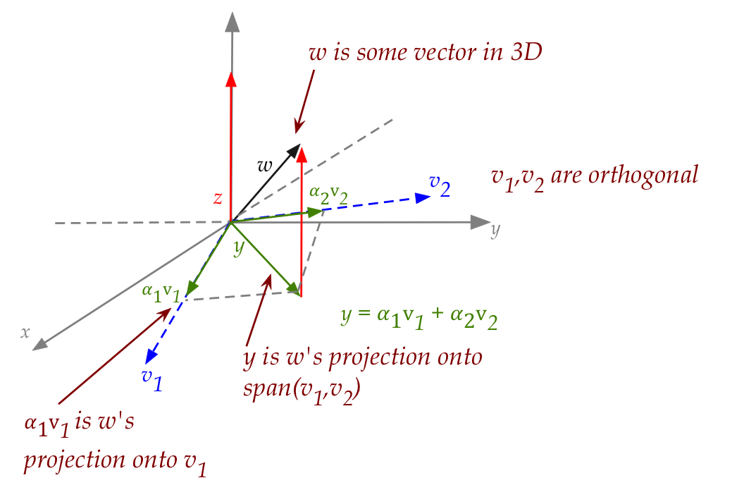
Let's make sense of this busy picture:
- Think of \({\bf w}\) as a regular 3D vector sticking out into
3D space.
- Next, let \({\bf v}_1\) and \({\bf v}_2\) be two
orthogonal vectors in the x-y plane.
- We want to ask: what's the projection of \({\bf w}\)
onto each of \({\bf v}_1\) and \({\bf v}_2\) and what do
those individual projections have to do with \({\bf y}\), the
projection of \({\bf w}\) on the span of the two vectors?
- The individual projections are:
$$\eqb{
\alpha_1 {\bf v}_1 \\
\alpha_2 {\bf v}_2 \\
}$$
where
$$\eqb{
\alpha_1 & \eql & \frac{{\bf w} \cdot {\bf v}_1}{{\bf v}_1 \cdot {\bf v}_1}\\
\alpha_2 & \eql & \frac{{\bf w} \cdot {\bf v}_2}{{\bf v}_2 \cdot {\bf v}_2}\\
}$$
- But the sum of these is exactly \({\bf y}\):
$$
{\bf y} \eql \alpha_1{\bf v}_1 + \alpha_2{\bf v}_2
$$
- Note: you cannot reconstruct the original vector \({\bf w}\)
knowing only the individual projections
\(\alpha_1{\bf v}_1\) and \(\alpha_2{\bf v}_2\).
- That's because \({\bf w}\) is not in the same space as
\({\bf v}_1\) and \({\bf v}_2\).
So, finally, let's look at the case when
\({\bf w}\) is in the span of
\({\bf v}_1\) and \({\bf v}_2\).
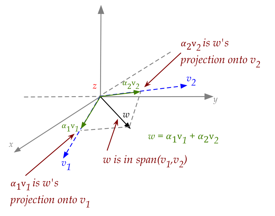
In this case:
- The individual projections add up to the original vector \({\bf w}\):
$$
{\bf w} \eql \alpha_1{\bf v}_1 + \alpha_2{\bf v}_2
$$
- Thus, when \({\bf w}\) is in the span of
\({\bf v}_1\) and \({\bf v}_2\),
we can fully reconstruct \({\bf w}\) knowing only the
individual projections on the basis vectors.
- Note: although we have used a basis for the x-y plane,
the above reasoning applies to any subspace and any orthogonal basis
for that subspace.
- Thus, in the general case we'd say that
$$
{\bf w} \eql \alpha_1{\bf v}_1 + \alpha_2{\bf v}_2
\; \ldots \; + \alpha_n{\bf v}_n
$$
where
$$
\alpha_i \eql \frac{{\bf w} \cdot {\bf v}_i}{{\bf v}_i \cdot {\bf v}_i}
$$
A further simplification when the basis is orthonormal:
- When the \({\bf v}_i\)'s are orthonormal, they have unit length
and so
$$
{\bf v}_i \cdot {\bf v}_i \eql |{\bf v}_i|^2 \eql 1.
$$
Which means
$$
\alpha_i \eql {\bf w} \cdot {\bf v}_i
$$
- Then
$$
{\bf w} \eql ({\bf w} \cdot {\bf v}_1) {\bf v}_1 +
\; \ldots \; + ({\bf w} \cdot {\bf v}_n) {\bf v}_n
$$
This is worth remembering: many applications use orthonormal bases.
Go to Part III