r.1 What are vectors and what do you do with them?
Let's start with: what are vectors and how did they come about?
- Vectors come about when we arrange for arithmetic operators to
apply simultaneously across a collection of numbers, as in
$$
(1,2,3) + (4,5,-6) \eql (5,7,-3)
$$
- Just by itself, such an extension of arithmetic operators
(to groups of numbers) might remain a mathematical
curiosity. However, when given the "right" geometric meaning,
it turns out to be startlingly useful (as we'll see throughout the course).
⇒
which is why we get the field of linear algebra
- So, a vector is an ordered collection of real numbers, such as
$$\eqb{
(1,2,3) & \eql & \mbox{ a 3-component or 3-dimensional vector} \\
(1.414, - 2.718) & \eql & \mbox{ a 2-dimensional vector} \\
(0,0,1,-2,6,1.1,10^{-6}) & \eql & \mbox{ a 7-dimensional vector} \\
}$$
- We define the following operations on vectors:
- Scalar multiplication: a real number that multiplies into
every component of a vector, e.g.,
$$\eqb{
4 (1,2,3) & \eql & (4\times 1, \; 4\times 2, \; 4\times 3) \\
& \eql & (4,8,12)
}$$
Let's get used to the seeing this symbolically:
$$\eqb{
\alpha {\bf u} & \eql & \alpha (u_1,\ldots,u_n) \\
& \eql & (\alpha u_1, \ldots, \alpha u_n)
}$$
- Vector addition (for vectors of the same dimension):
$$\eqb{
(1,2,3) + (4,5,-6) & \eql & (1+4, \; 2+5, \; 3-6) \\
& \eql & (5,7,-3)
}$$
Symbolically:
$$\eqb{
{\bf u} + {\bf v} & \eql &
(u_1,u_2,\ldots,u_n) + (v_1,v_2,\ldots,v_n) \\
& \eql & (u_1+v_1, \; u_2+v_2, \; \ldots, \;u_n+v_n)
}$$
- Vector dot-product (again, with the same
dimension), which produces a single number as a result:
$$\eqb{
(1,2,3) \cdot (4,5,-6) & \eql & 1\times 4 \plss 2\times 5 \plss 3\times -6\\
& \eql & -4 \;\;\;\;\;\; \mbox{ (a number)}
}$$
Symbolically:
$$\eqb{
{\bf u} \cdot {\bf v} & \eql &
(u_1,u_2,\ldots,u_n) \cdot (v_1,v_2,\ldots,v_n) \\
& \eql & u_1v_1 + u_2v_2 + \ldots + u_nv_n
}$$
- Why were these operations defined in this way?
- Scalar multiplication because "stretching" is what
gives us linear combinations, the foundation of the theory.
- Addition because, after stretching, addition via parallelogram
is how we "reach" other vectors.
- Dot-product because that'll give us the angle (kind of) between
two vectors, which will be useful for orthogonality and vector-similarity.
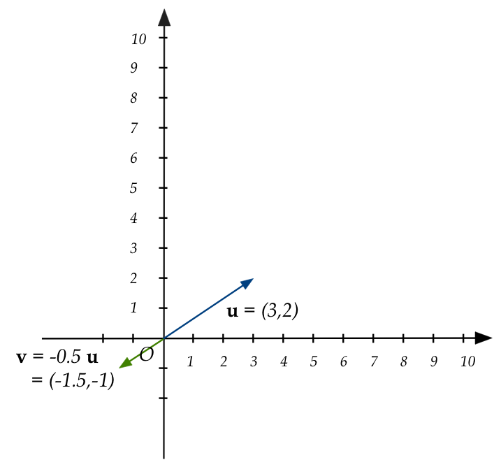
- The geometry of scalar multiplication = "stretching" (or shrinking)
- The geometric interpretation of addition:
\( \bf{w} = \bf{u} + \bf{v} \)
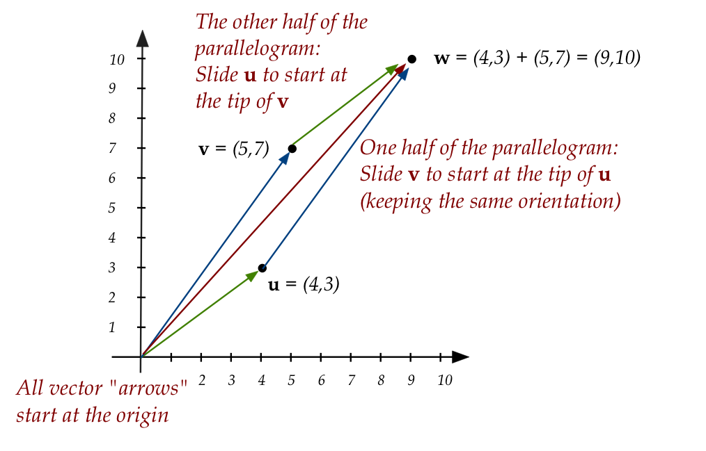
Recall:
- All arrows representing vectors start (have their tail)
at the origin.
- We slide one vector to make a parallelogram only for the sake
of illustration. Thus, the upper two arrows that do not start at the
origin are only to show how
addition produces the result (red) vector.
- And the even more important interpretation of "stretch and
add", for example: \(\bf{w} = 1.5 \bf{u} + 2{\bf v} \)
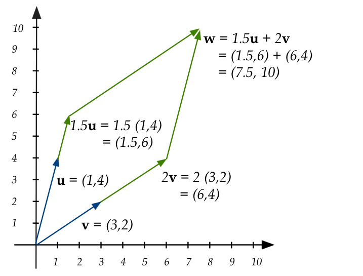
- Stretch \(\bf{u}\) by 1.5, stretch \(\bf{v}\) by 2.
- This results in two stretched vectors \(1.5\bf{u}\) and
\(2\bf{v}\).
- The stretched vectors are then added: this is what we
mean by a linear combination of vectors.
- Let's look at a 3D example with two vectors
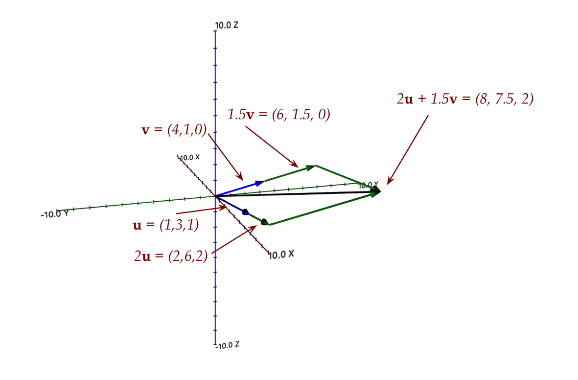
Here:
- The two vectors are: \({\bf u}=(1,3,1), \; {\bf v}=(4,1,0)\)
- The stretched addition is a parallelogram:
$$\eqb{
2{\bf u} + 1.5{\bf v} & \eql & 2(1,3,1) \plss 1.5(4,1,0) \\
& \eql & (2,6,2) \plss (6,1.5,0) \\
& \eql & (8,7.5,2)
}$$
- And one with three 3D vectors:
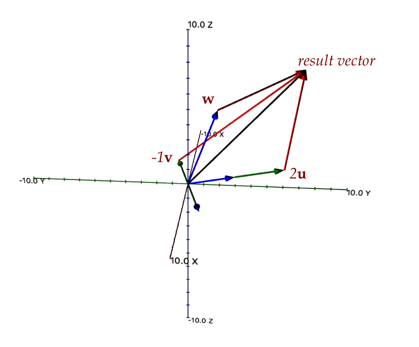
Here:
- \({\bf u}=(1,3,1), \; {\bf v}=(4,1,0), \; {\bf w}=(3,2,6)\)
- The stretched addition is a 3D-parallelogram (parallelpiped):
$$\eqb{
2{\bf u} - {\bf v} + {\bf w}
& \eql & 2(1,3,1) \miss (4,1,0) \plss (3,2,6)\\
& \eql & (1,7,8)
}$$
Notation for many vectors:
- All the examples above had two or three vectors.
- Often, we need to work with several vectors.
- We'll use subscripts. For example, for a collection of 5 vectors:
$$
{\bf v}_1, \; {\bf v}_2, \; {\bf v}_3, \; {\bf v}_4, \; {\bf v}_5,
$$
- What's important: even though these are subscripted, they
themselves have components, for example:
$$\eqb{
{\bf v}_1 & \eql & (1,2,3) \\
{\bf v}_2 & \eql & (4,5,6) \\
}$$
In this case, you need to track subscripts carefully to see
what the meaning is in the current context.
- Suppose \({\bf v}_1, {\bf v}_2,\ldots, {\bf v}_n\)
are a collection of vectors:
- Next, let \(x_1,x_2,\ldots, x_n\) be \(n\) real numbers.
- Then a linear combination (stretches-plus-addition)
produces a vector, which we write as:
$$
{\bf w} \eql x_1 {\bf v}_1 + x_2 {\bf v}_2 + \ldots +
x_n {\bf v}_n
$$
- For example:
- Suppose:
$$\eqb{
{\bf v}_1 & \eql & (1,3,1) \\
{\bf v}_2 & \eql & (4,1,0) \\
{\bf v}_3 & \eql & (3,2,6)
}$$
- Then, suppose
$$\eqb{
x_1 & \eql & 2\\
x_2 & \eql & -1\\
x_3 & \eql & 1\\
}$$
- Then the linear combination
\(x_1 {\bf v}_1 + x_2 {\bf v}_2 + x_3 {\bf v}_3\)
turns out to be:
$$\eqb{
x_1 {\bf v}_1 + x_2 {\bf v}_2 + x_3 {\bf v}_3
& \eql &
2 (1,3,1) \miss (4,1,0) \plss (3,2,6) \\
& \eql &
(2,6,2) \miss (4,1,0) \plss (3,2,6) \\
& \eql & (2-4+3,\;\; 6-1+2, \;\; 2-0+6)\\
& \eql & (1,7,8)
}$$
- Let's rewrite that last step differently:
$$\eqb{
x_1 {\bf v}_1 + x_2 {\bf v}_2 + x_3 {\bf v}_3
& \eql &
2 (1,3,1) \miss (4,1,0) \plss (3,2,6) \\
& \eql &
(2*1 - 4 + 3, \;\; 2*3 - 1 + 2, \;\; 2*1 - 0 + 6)
}$$
Notice:
- Rather than complete the scalar multiplication, we leave
the individual multiplications and add across the dimensions of
each vector.
- This is important to notice because, consider this:
- Suppose we have three 3D vectors:
$$\eqb{
{\bf u} & \eql & (u_1, u_2, u_3) \\
{\bf v} & \eql & (v_1, v_2, v_3) \\
{\bf w} & \eql & (w_1, w_2, w_3) \\
}$$
- Here, we're just using letters \({\bf u},{\bf v},{\bf w}\)
to avoid double-subscripting.
- Now suppose we have three scalars \(\alpha, \beta, \gamma\).
- Then, the linear combination
\(\alpha{\bf u} + \beta {\bf v} + \gamma{\bf w}\) becomes
$$\eqb{
\alpha{\bf u} + \beta {\bf v} + \gamma{\bf w}
& \eql &
\alpha (u_1,u_2,u_3) + \beta (v_1, v_2, v_3) + \gamma (w_1, w_2, w_3)\\
& \eql &
(\alpha u_1 + \beta v_1 + \gamma w_1, \;
\alpha u_2 + \beta v_2 + \gamma w_2, \;
\alpha u_3 + \beta v_3 + \gamma w_3)
}$$
- This is easier to see if we write the vectors in column format:
$$\eqb{
\alpha{\bf u} + \beta {\bf v} + \gamma{\bf w}
& \eql &
\alpha \vecthree{u_1}{u_2}{u_3}
\plss \beta \vecthree{v_1}{v_2}{v_3}
\plss \gamma \vecthree{w_1}{w_2}{w_3} \\
& \eql &
\vecthree{\alpha u_1 + \beta v_1 + \gamma w_1}{\alpha u_2 + \beta v_2 + \gamma w_2}{\alpha u_3 + \beta v_3 + \gamma w_3}
}$$
- These last few points about notation are really important
to be comfortable with. Write down a few examples of your own to clarify.
About that "column style" of writing a vector:
- From here, whenever you "think" vector, you should think
"column" style:
- We write \({\bf v} = (1,2,3)\) instead of
$$
{\bf v} \eql \vecthree{1}{2}{3}
$$
only for the sake of compactness or convenience in text.
- Otherwise the text will look weird,
\({\bf v} \eql \vecthree{1}{2}{3}\), if we
embed the column format into free-flowing paragraph text.
- Sometimes, we'll emphasize the "row" style when it's useful
by explicitly transposing the column into a row vector:
$$
{\bf v}^T \eql \mat{1 & 2 & 3}
$$
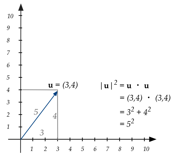
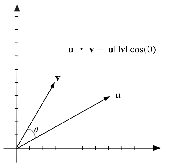
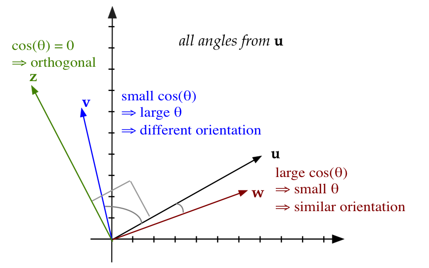
r.2 Dot products, lengths, angles, orthogonal vectors
The dot-product conveniently gives us two nice results:
r.3 Matrix-vector multiplication and what it means
Let's go back to the linear combination of three 3D vectors from
earlier:
$$\eqb{
\alpha \vecthree{u_1}{u_2}{u_3}
\plss \beta \vecthree{v_1}{v_2}{v_3}
\plss \gamma \vecthree{v_1}{v_2}{v_3}
& \eql &
\vecthree{\alpha u_1 + \beta v_1 + \gamma w_1}{\alpha u_2 + \beta v_2 + \gamma w_2}{\alpha u_3 + \beta v_3 + \gamma w_3}
}$$
- Think of the left side as the linear combination and the
right side as the vector that results from the linear combination.
- Matrices came about by visually
reorganizing the left side into
$$\eqb{
\alpha \vecthree{u_1}{u_2}{u_3}
\plss \beta \vecthree{v_1}{v_2}{v_3}
\plss \gamma \vecthree{v_1}{v_2}{v_3}
& \eql &
\mat{
u_1 & v_1 & w_1 \\
u_1 & v_2 & w_2 \\
u_1 & v_3 & w_3 \\
}
\vecthree{\alpha}{\beta}{\gamma}
}$$
- Since it's the same left-side (just visually) reorganized, it must equal the
original right side:
$$
\mat{
u_1 & v_1 & w_1 \\
u_2 & v_2 & w_2 \\
u_3 & v_3 & w_3 \\
}
\vecthree{\alpha}{\beta}{\gamma}
\eql
\vecthree{\alpha u_1 + \beta v_1 + \gamma w_1}{\alpha u_2 + \beta v_2 + \gamma w_2}{\alpha u_3 + \beta v_3 + \gamma w_3}
$$
- Let's give each of these names:
$$\eqb{
{\bf A} & \defn &
\mat{
u_1 & v_1 & w_1 \\
u_1 & v_2 & w_2 \\
u_1 & v_3 & w_3 \\
} \\
{\bf x} & \defn & \vecthree{\alpha}{\beta}{\gamma}\\
{\bf b} & \defn &
\vecthree{\alpha u_1 + \beta v_1 + \gamma w_1}{\alpha u_2 + \beta v_2 + \gamma w_2}{\alpha u_3 + \beta v_3 + \gamma w_3}
}$$
- Then, written in these symbols, we have
$$
{\bf Ax} \eql {\bf b}
$$
- What we have is a "matrix times a vector gives a vector".
⇒
The matrix \({\bf A}\) times vector \({\bf x}\) gives the vector
\({\bf b}\)
There are two meanings of \({\bf Ax} = {\bf b}\).
Let's look at the first one, what we just did above:
- Here, \({\bf x}\) is only incidentally a vector
(because it looks like one).
- The only thing that matters about \({\bf x}\) is that
it contains the scalars in the linear combination.
- And the linear combination of what? The columns of \({\bf
A}\), each of which is a vector.
- The result is the right side vector, remembering that
a linear combination of vectors is a vector.
- So, when we "unpack" \({\bf Ax} = {\bf b}\), the left side
unpacks into:
$$
\mat{
u_1 & v_1 & w_1 \\
u_2 & v_2 & w_2 \\
u_3 & v_3 & w_3 \\
}
\vecthree{\alpha}{\beta}{\gamma}
\eql
\alpha \vecthree{u_1}{u_2}{u_3}
\plss \beta \vecthree{v_1}{v_2}{v_3}
\plss \gamma \vecthree{v_1}{v_2}{v_3}
$$
- Whereas the right side is the result vector (of the linear combination):
$$
\vecthree{\alpha u_1 + \beta v_1 + \gamma w_1}{\alpha u_2 + \beta v_2 + \gamma w_2}{\alpha u_3 + \beta v_3 + \gamma w_3}
$$
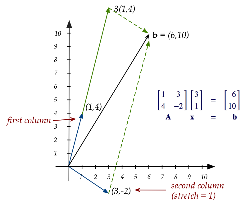
- Let's look at a 2D example:
- First, examine the linear combination
$$
3 \vectwo{1}{4} \plss 1 \vectwo{3}{-2} \eql \vectwo{6}{10}
$$
- We've learned that the left side can be written in matrix
form as:
$$\eqb{
\mat{1 & 3\\
4 & -2}
\vectwo{3}{1}
& \eql & \vectwo{6}{10}\\
{\bf A} \;\;\;\;\;\;\;\; {\bf x} \;\;\;
& \eql & \;\;\;\; {\bf b}
}$$
- Now let's draw these:
- Let's write "linear combination of columns"
generally for the case of \(n\) dimensions to see what it looks like:
$$\eqb{
{\bf Ax} & \eql &
\mat{\vdots & \vdots & \cdots & \vdots\\
{\bf c}_1 & {\bf c}_2 & \cdots & {\bf c}_n\\
\vdots & \vdots & \cdots & \vdots}
\mat{x_1 \\ x_2 \\ \vdots \\ x_n}\\
& \eql &
x_1 {\bf c}_1 \plss x_2 {\bf c}_2 \plss \ldots \plss
x_n {\bf c}_n
}$$
Thus, the \({\bf x}\) vector, using its component values (which
are numbers) creates a linear combination of the columns of
\({\bf A}\).
- When we ask whether there is an \({\bf x}\) vector
such that \({\bf Ax}={\bf b}\), we are asking whether there
is some linear combination of the column vectors to produce
the vector \({\bf b}\).
The second interpretation: a matrix transforms a vector
- When seeing
$$\eqb{
\mat{1 & 3\\
4 & -2}
\vectwo{3}{1}
& \eql & \vectwo{6}{10}\\
{\bf A} \;\;\;\;\;\;\;\; {\bf x} \;\;\;
& \eql & \;\;\;\; {\bf b}
}$$
think of
- \({\bf x}\) is just some vector
$$
{\bf x} \eql \vectwo{3}{1}
$$
- \({\bf A}\) as a matrix that "does something" to \({\bf x}\)
to produce another vector \({\bf b}\).
- Pictorially:
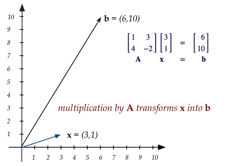
- Here, we've actually drawn \({\bf x}\) as a vector.
There is one more useful way to view matrix-vector multiplication:
- Suppose we think of the matrix \({\bf A}\)'s rows as
vectors.
- Then, the calculation of the resulting vector
\({\bf b}\)'s components can be written as a row of
\({\bf A}\) times \({\bf x}\).
- In our 2D example, the first element of \({\bf b}\) is:
$$
\mat{{\bf 1} & {\bf 3}\\
4 & -2}
\vectwo{{\bf 3}}{{\bf 1}}
\eql \vectwo{{\bf 1}\times {\bf 3} \; + \; {\bf 3}\times {\bf 1}}{10}
\eql \vectwo{{\bf 6}}{10}
$$
and the second element of \({\bf b}\) is computed by multiplying
the second row of \({\bf A}\) times \({\bf x}\):
$$
\mat{1 & 3\\
{\bf 4} & {\bf -2}}
\vectwo{{\bf 3}}{{\bf 1}}
\eql \vectwo{6}{{\bf 4}\times {\bf 3} \; {\bf -} \; {\bf
2}\times {\bf 1}}
\eql \vectwo{6}{{\bf 10}}\\
$$
- But the row-of-\({\bf A}\) times \({\bf x}\) can be written
as a dot product. For example:
$$
\mat{1 & 3\\
{\bf 4} & {\bf -2}}
\vectwo{{\bf 3}}{{\bf 1}}
\eql \vectwo{6}{(4,-2)\cdot (3,1)}
\eql \vectwo{6}{{\bf 10}}\\
$$
- Suppose we give names to the rows of \({\bf A}\). Then:
$$
\mat{\cdots & {\bf r}_1 & \cdots\\
\cdots & {\bf r}_2 & \cdots}
{\bf x}
\eql \vectwo{{\bf r}_1 \cdot {\bf x}}{{\bf r}_2 \cdot {\bf x}}
$$
- This works for any size matrix-vector multiplication:
$$
\mat{\cdots & {\bf r}_1 & \cdots\\
\cdots & {\bf r}_2 & \cdots\\
\vdots & \vdots & \vdots\\
\cdots & {\bf r}_m & \cdots}
{\bf x}
\eql
\mat{ {\bf r}_1 \cdot {\bf x} \\
{\bf r}_2 \cdot {\bf x} \\
\vdots \\
{\bf r}_m \cdot {\bf x}}
$$
- This interpretation of matrix-vector multiplication does not
come with geometric meaning.
r.4 Solving \({\bf Ax} = {\bf b}\) exactly and approximately
Let's start with some equations:
$$
\eqb{
x_1 + 3x_2 & = 7.5 \\
4x_1 + 2x_2 & = 10 \\
}
$$
- In "vector stretch" form, they become:
$$
x_1 \vectwo{1}{4} + x_2 \vectwo{3}{2} \eql \vectwo{7.5}{10}
$$
- So, asking to solve the equations is the same as asking "is
there a linear combination (values of \(x_1,x_2\)) such that
the linear combintion on left yields the vector on the right?"
-
- Thus \(x_1=1.5, \;\; x_2=2\) is a solution:
$$
1.5 \vectwo{1}{4} + 2 \vectwo{3}{2} \eql \vectwo{7.5}{10}
$$
Next, let's examine a case where no solution exists:
$$
\eqb{
x_1 + 3x_2 & = 7.5 \\
2x_1 + 6x_2 & = 10 \\
}
$$
- In "vector stretch" form, this is asking if there exist
scalars \(x_1,x_2\) such that:
$$
x_1 \vectwo{1}{2} + x_2 \vectwo{3}{6} \eql \vectwo{7.5}{10}
$$
- Pictorially, it's easy to see that there's no solution:
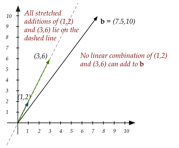
- Digging a bit deeper,
notice that the vector \((3,6)\), which is the second column
is in fact a multiple of the first column \((1,2)\).
- Thus, it so happens that
$$
3 \vectwo{1}{2} - \vectwo{3}{6} \eql \vectwo{0}{0}
$$
- In other words, the special equation
$$
x_1 \vectwo{1}{2} + x_2 \vectwo{3}{6} \eql \vectwo{0}{0}
$$
has a non-zero solution \((x_1,x_2) = (3,-1)\).
- This means that the two columns are not independent (by the
definition of linear independence).
- Thus, the matrix
$$
\mat{1 & 3\\
2 & 6}
$$
is not full-rank.
- As an exercise: work out the RREF to see that there's only
one pivot.
Now, let's look at the case where multiple solutions exist:
$$
\eqb{
x_1 + 3x_2 & = 4 \\
2x_1 + 6x_2 & = 8 \\
}
$$
- In "stretch form":
$$
x_1 \vectwo{1}{2} + x_2 \vectwo{3}{6} \eql \vectwo{4}{8}
$$
- Pictorially:
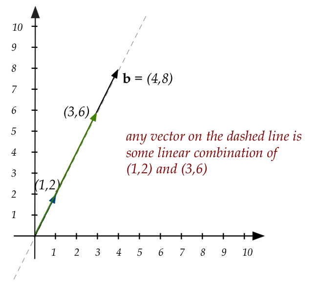
- So, for example \(x_1=1, x_2=1\) is one solution.
- So are \(x_1=0.7, x_2=1.1\), \(x_1=0.667, x_2=1.111\),
and countless others.
Let's examine a 3D example:
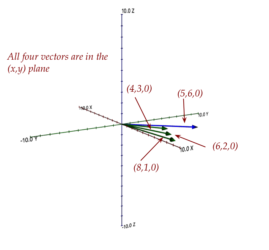
What do we do when no solution is possible?
- Consider \({\bf Ax}={\bf b}\) and \({\bf A}\)'s columns:
$$
{\bf A} \eql
\mat{\vdots & \vdots & \ldots & \vdots\\
{\bf c}_1 & {\bf c}_2 & \ldots & {\bf c}_n\\
\vdots & \vdots & \ldots & \vdots}
$$
- In general, if \({\bf Ax}={\bf b}\) does not have
a solution, it means right-side vector \({\bf
b}\) is not in the span of the columns of \({\bf A}\).
- Recall: the span of a set of vectors is all the vectors you
can reach by linear combinations.
- Thus, there is no linear combination such that
$$
x_1 {\bf c}_1 + x_2{\bf c}_2 + \ldots + x_n{\bf c}_n
\eql {\bf b}
$$
- Suppose we were to seek a "next best" or approximate
solution \(\hat{\bf x}\).
- The first thing to realize is that an approximate
solution is still a linear combination of the columns:
$$
\hat{x}_1 {\bf c}_1 + \hat{x}_2{\bf c}_2 + \ldots
+ \hat{x}_n{\bf c}_n
\eql ?
$$
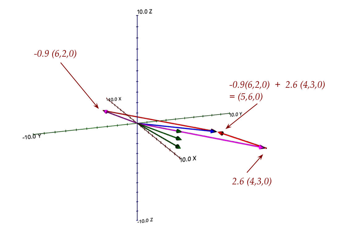
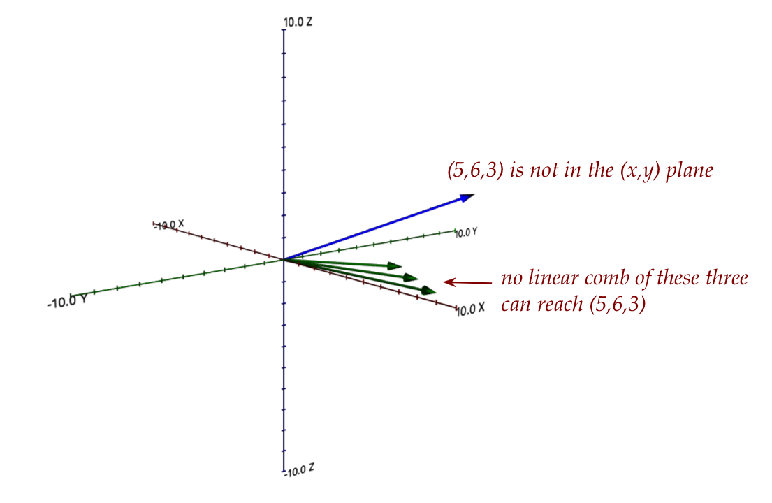
- Thus, in our example, we seek
$$
\hat{x}_1 \vecthree{6}{2}{0} + \hat{x}_2\vecthree{4}{3}{0}
+ \hat{x}_3\vecthree{8}{1}{0}
$$
that's closest to the desired target \((5,6,3)\).
- Our example provides an intuition:
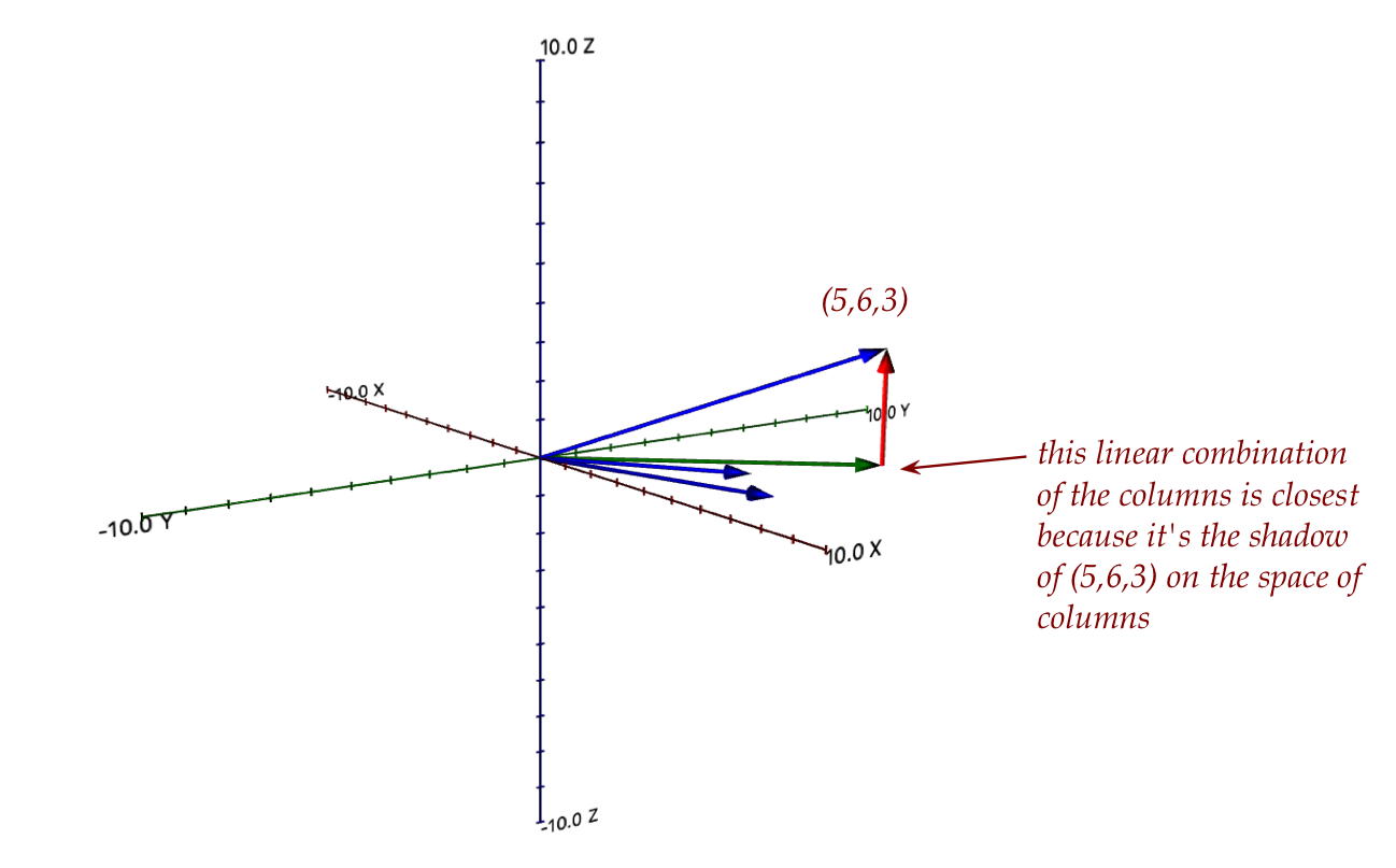
- The difference vector between the "closest" and \({\bf b}\)
is perpendicular to every vector in the span of the columns.
- This is what the least-squares method exploits.
- The least squares method:
Suppose
$$
{\bf y} \eql \mbox{ the closest vector in the colspan}
$$
Let
$$\eqb{
{\bf z} & \eql & \mbox{ the difference vector}\\
& \eql & {\bf b} - {\bf y}
}$$
Here, \({\bf z}\) is the red vector in the diagram above.
-
Since \({\bf z}\) is perpendicular to the plane containing the
columns, it's perpendicular to the columns themselves:
$$\eqb{
{\bf c}_1 \cdot {\bf z} \eql 0 \\
{\bf c}_2 \cdot {\bf z} \eql 0 \\
}$$
- The rest of least squares stems from the observation that
the columns of \({\bf A}\) are rows of \({\bf A}^T\):
- If we were to multiply \({\bf A}^T\) into \({\bf z}\):
$$
{\bf A}^T {\bf z}
\eql
\mat{\ldots & {\bf c}_1 & \ldots\\
\ldots & {\bf c}_2 & \ldots\\
\vdots & \vdots & \vdots\\
\ldots & {\bf c}_n & \ldots}
\eql
\mat{ {\bf c}_1 \cdot {\bf z} \\
{\bf c}_2 \cdot {\bf z} \\
\vdots \\
{\bf c}_n \cdot {\bf z}}
\eql
\mat{ 0 \\ 0\\ 0\\ 0}
$$
- Now plug in
$$
{\bf y} \eql {\bf A} \hat{{\bf x}}
$$
in
$$
{\bf z} \eql {\bf b} - {\bf y}
$$
and do the algebra to get
$$
{\bf A}^T {\bf b} - {\bf A}^T {\bf A}\hat{\bf x} \eql {\bf 0}
$$
after which we get
$$
\hat{\bf x}
\eql
({\bf A}^T {\bf A})^{-1}
{\bf A}^T {\bf b}
$$
provided the inverse exists.
Go to Part II