Module 2: Sorting
Introduction
The Sorting problem:
- Simple version: given a collection of elements, sort them.
- Practical issues:
- How is the "collection" given?
Array? File? Via a database?
- What kinds of "elements"?
Integers? Strings? Objects that know to compare themselves?
- What is known about the data?
Random? Almost sorted? Small-size? Large-size?
- Sort order?
Increasing? Decreasing?
- What about the output?
Sort in place? Return an array of sort-indices?
Let's start by looking at a classic algorithm: BubbleSort
The code: (source file)
public class BubbleSort {

  public void sortInPlace (int[] data)
  {
    // Key idea: Bubble smallest element, then next smallest etc.

    // 1. For positions i=0,...,length-1, find the element that should be at position i
    for (int i=0; i < data.length-1; i++){

      // 1.1 Scan all elements past i starting from the end:
      for (int j=data.length-1; j > i; j--) {

        // 1.1.1 If a pair of consecutive elements is out of
        //       order, swap the elements:
        if (data[j-1] > data[j])
          swap (data, j-1, j);

      }

    }

  }

  public void sortInPlace (Comparable[] data)
  {
    for (int i=0; i < data.length-1; i++){
      for (int j=data.length-1; j > i; j--) {
        // Notice the use of the compareTo method:
        if (data[j-1].compareTo (data[j]) > 0)
          swap (data, j-1, j);
      }
    }
  }

  public int[] createSortIndex (int[] data)
  {
    // 1. Create space for a sort index:
    int[] index = new int [data.length];

    // 2. Initialize to current data:
    for (int i=0; i < data.length; i++)
      index[i] = i;

    // 3. Sort indices by comparing data:
    for (int i=0; i < data.length-1; i++){
      for (int j=data.length-1; j > i; j--) {
        if (data[index[j-1]] > data[index[j]])
          swap (index, j-1, j);
      }
    }
    return index;
  }

  public int[] createSortIndex (Comparable[] data)
  {
    // ...
  }

  void swap (int[] data, int i, int j)
  {
    int temp = data[i];
    data[i] = data[j];
    data[j] = temp;
  }


  void swap (Comparable[] data, int i, int j)
  {
    // ...
  }


  public static void main (String[] argv)
  {

    // Testing ...

  }

}
Note:
- We could have written the code a little differently:
(source file)
public class BubbleSort2 {

  void bubble (int[] data, int startingPosition)
  {
    // Swap down the element that belongs in "startingPosition".
    for (int j=data.length-1; j > startingPosition; j--) {
      if (data[j-1] > data[j])
        swap (data, j-1, j);
      }
  }


  public void sortInPlace (int[] data)
  {
    // Key idea: Bubble smallest element, then next smallest etc.

    // 1. For positions i=0,...,length-1, find the element that belongs at i:
    for (int i=0; i < data.length-1; i++){
      bubble (data, i);
    }
  }

  // ...

}
This is more readable, but costs an extra method call in each iteration.
- To optimize, we could avoid the procedure call to swap:
  public void sortInPlace (int[] data)
  {
    for (int i=0; i < data.length-1; i++){
      for (int j=data.length-1; j > i; j--) {
        if (data[j-1] > data[j]) {
          int temp = data[j-1];
          data[j-1] = data[j];
          data[j] = temp;
        }
      }
    }
  }
- What is the complexity of BubbleSort?
- In the i-th scan we perform (n-i) comparisons.
- Hence: (n-1) + (n-2) + ... + 1
- This gives: O(n2).
- Also, observe:
- Some comparisons result in the extra cost of a swap.
- The same number of comparisons is performed no matter what
the data.
Thus, an already-sorted file will still take
O(n2) time.
Recursion: a review
Review recursion from
CS-133, Module 4
QuickSort
In-Class Exercise 2.1:
Download this template
and implement the QuickSort algorithm:
- You have already implemented partitioning: copy over that code.
- The basic quicksort recursion, along with test-code is in the template.
- When the input array is already sorted, how many comparisons
are made?
You will also need UniformRandom.java.
Pseudocode:
  Algorithm: quickSort (data)
  Input: data - an array of size n
  1.  quickSortRecursive (data, 0, n-1)


  Algorithm: quickSortRecursive (data, L, R)
  Input: data - an array of size n with a subrange specified by L and R
  1.   if L ≥ R
  2.       return
  3.   endif

       // Partition the array and position partition element correctly.
  4.   p = partition (data, L, R)

  5.   quickSortRecursive (data, L, p-1)    // Sort left side
  6.   quickSortRecursive (data, p+1, R)    // Sort right side
Let's look at a sample execution on a 10-character array
"N G Q S K V S K W I"
Here is the trace:
 N G Q S K V S K W I     Start

 K G I K N V S S W Q     L=0 R=9 P=4 next: [0,3]  [5,9]
 ^                 ^

 K G I K N V S S W Q     L=0 R=3 P=3 next: [0,2]  [4,3]
 ^     ^

 I G K K N V S S W Q     L=0 R=2 P=2 next: [0,1]  [3,2]
 ^   ^

 G I K K N V S S W Q     L=0 R=1 P=1 next: [0,0]  [2,1]
 ^ ^

 G I K K N V S S W Q     L=0 R=0 No partition
 ^

 G I K K N V S S W Q     L=2 R=1 No partition
   ^ ^

 G I K K N V S S W Q     L=3 R=2 No partition
     ^ ^

 G I K K N V S S W Q     L=4 R=3 No partition
       ^ ^

 G I K K N Q S S V W     L=5 R=9 P=8 next: [5,7]  [9,9]
           ^       ^

 G I K K N Q S S V W     L=5 R=7 P=5 next: [5,4]  [6,7]
           ^   ^

 G I K K N Q S S V W     L=5 R=4 No partition
         ^ ^

 G I K K N Q S S V W     L=6 R=7 P=7 next: [6,6]  [8,7]
             ^ ^

 G I K K N Q S S V W     L=6 R=6 No partition
             ^

 G I K K N Q S S V W     L=8 R=7 No partition
               ^ ^

 G I K K N Q S S V W     L=9 R=9 No partition
                   ^
In-Class Exercise 2.2:
Write pseudocode for a non-recursive (iterative) implementation of
quicksort, assuming that the method for partitioning
already exists. Show what the stack contains after
the fifth step in your loop.
Next, we will examine some variations of QuickSort:
- Different ways to select a partitioning element.
- Different partitioning algorithms.
- Additional optimizations to the basic code.
First, observe what happens with the following test data:
"A B C D E F G H I J":
 A B C D E F G H I J     L=0 R=9 P=0 next: [0,-1]  [1,9]
 ^                 ^

 A B C D E F G H I J     L=0 R=-1 No partition
 ^

 A B C D E F G H I J     L=1 R=9 P=1 next: [1,0]  [2,9]
   ^               ^

 A B C D E F G H I J     L=1 R=0 No partition
 ^ ^

 A B C D E F G H I J     L=2 R=9 P=2 next: [2,1]  [3,9]
     ^             ^

 A B C D E F G H I J     L=2 R=1 No partition
   ^ ^

 A B C D E F G H I J     L=3 R=9 P=3 next: [3,2]  [4,9]
       ^           ^

 A B C D E F G H I J     L=3 R=2 No partition
     ^ ^

 A B C D E F G H I J     L=4 R=9 P=4 next: [4,3]  [5,9]
         ^         ^

 A B C D E F G H I J     L=4 R=3 No partition
       ^ ^

 A B C D E F G H I J     L=5 R=9 P=5 next: [5,4]  [6,9]
           ^       ^

 A B C D E F G H I J     L=5 R=4 No partition
         ^ ^

 A B C D E F G H I J     L=6 R=9 P=6 next: [6,5]  [7,9]
             ^     ^

 A B C D E F G H I J     L=6 R=5 No partition
           ^ ^

 A B C D E F G H I J     L=7 R=9 P=7 next: [7,6]  [8,9]
               ^   ^

 A B C D E F G H I J     L=7 R=6 No partition
             ^ ^

 A B C D E F G H I J     L=8 R=9 P=8 next: [8,7]  [9,9]
                 ^ ^

 A B C D E F G H I J     L=8 R=7 No partition
               ^ ^

 A B C D E F G H I J     L=9 R=9 No partition
                   ^
Choosing a partitioning element:
- Easy choices: leftmost element, or rightmost element.
- Using an extreme element can cause the worst partitioning
repeatedly if the array is sorted.
- Better choices:
- Pick a random element.
- Pick the median of: left, right and center elements.
A random partitioning element:
  void quickSortRecursive (int[] data, int left, int right)
  {
    if (left < right) {
      // 1. Swap a random element into the leftmost position:
      int k = (int) UniformRandom.uniform ( (int) left+1, (int) right );
      swap (data, k, left);

      // 2. Partition:
      int partitionPosition = leftPartition (data, left, right);

      // 3. Sort left side:
      quickSortRecursive (data, left, partitionPosition-1);

      // 4. Sort right side:
      quickSortRecursive (data, partitionPosition+1, right);
    }
  }
Note:
- Minor detail: what happens when left+1 == right?
- Assume: random generator returns values inclusive of range-ends.
- Value returned is right - still works.
- This type of detail, while not essential to explaining an
algorithm, is extremely important in practice.
- If a "right-partition" is being used: swap random element into
rightmost position.
- It's possible to show: probability of poor performance with
randomization is very small.
Using the median approach:
  int pickMedian3 (int[] data, int a, int b, int c)
  {
    // Return the index of the middle value among data[a], data[b] and data[c].
  }

  void quickSortRecursive (int[] data, int left, int right)
  {
    if (left < right) {
      // 1. Pick the median amongst the left, middle and right elements
      //    and swap into leftmost position:
      int k = pickMedian3 (data, left, (left+right)/2, right);
      swap (data, k, left);

      // 2. Partition:
      int partitionPosition = leftPartition (data, left, right);

      // 3. Sort left side:
      quickSortRecursive (data, left, partitionPosition-1);

      // 4. Sort right side:
      quickSortRecursive (data, partitionPosition+1, right);

      // Partition element is already in the correct place.
    }
  }
In-Class Exercise 2.3:
Implement the median approach in your QuickSort algorithm.
Next, we will consider different partitioning ideas:
- Bidirectional partitioning:
- Recall: in bidirectional partitioning two cursors start at
the ends and move towards each other.
- Key idea:
- What's left of Left-Cursor is less than the partition element.
- What's right of Right-Cursor is larger than the partition element.
- If condition is violated, swap.
- Example: (LC = Left-Cursor, RC = Right-Cursor)
 K G I L N V B E B Q     LC=1 RC=9   Move RC left
   ^               ^

 K G I L N V B E B Q     LC=1 RC=8   Move LC right
   ^             ^

 K G I L N V B E B Q     LC=2 RC=8   Move LC right
     ^           ^

 K G I L N V B E B Q     LC=3 RC=8   Swap
       ^         ^

 K G I B N V B E L Q     LC=4 RC=7   Swap
         ^     ^

 K G I B E V B N L Q     LC=5 RC=6   Swap
           ^ ^

 K G I B E B V N L Q     LC=6 RC=5   Swap partition element
           ^ ^

 B G I B E K V N L Q     LC=6 RC=5   Partition complete
           ^ ^
- Pseudocode:
  Algorithm: leftBidirectionalPartition (data, left, right)
  Input: data array, indices left and right.

      // The partitioning element is the leftmost element:
  1.  partitionElement = data[left];

      // Start bidirectional scan from next-to-left, and right end.
  2.  LC = left+1;  RC = right;

      // Scan until cursors cross.
  3.  while (true)

        // As long as elements to the right are larger, skip over them:
  4.    while data[RC] > partitionElement
          RC = RC - 1;

        // As long as elements on the left are smaller, skip over them:
  5.    while (LC <= right) and (data[LC] < partitionElement)
          LC = LC + 1;

        // We've found the first pair to swap:
  6.    if (LC < RC)
  7.      Swap elements at positions LC and RC;
  8.      LC = LC + 1;    RC = RC - 1;
  9.    else
          // Otherwise, if the cursors cross, we're done.
  10.     break out of loop;
  11.   endif

  12. endwhile

  13. Swap RC-th element with leftmost.

  14. return RC;

  Output: new position of partition element
In-Class Exercise 2.4:
In line 4 above, why don't we need to check whether RC
becomes negative?
- Unidirectional partitioning:
- Two cursors move in the same direction.
- Key idea:
- What's left of Left-Cursor is less than the partition element.
- Right-Cursor sweeps whole array looking for "smaller"
elements to swap behind Left-Cursor.
- Example: (LC = Left-Cursor, RC = Right-Cursor)
 K G I L N V B E B Q     LC=1 RC=1   Swap
   ^

 K G I L N V B E B Q     LC=2 RC=2   Swap
     ^

 K G I L N V B E B Q     LC=2 RC=3
     ^

 K G I L N V B E B Q     LC=2 RC=4
     ^   ^

 K G I L N V B E B Q     LC=2 RC=5
     ^     ^

 K G I L N V B E B Q     LC=2 RC=6   Swap
     ^       ^

 K G I B N V L E B Q     LC=3 RC=7   Swap
       ^       ^

 K G I B E V L N B Q     LC=4 RC=8   Swap
         ^       ^

 K G I B E B L N V Q     LC=5 RC=9
           ^       ^

 K G I B E B L N V Q     LC=5 RC=9   Swap partition element
           ^       ^

 B G I B E K L N V Q     LC=5 RC=9   Partition complete
           ^       ^
- Pseudocode:
  Algorithm: leftUnidirectionalPartition (data, left, right)
  Input: data array, indices left and right.

      // The partitioning element is the leftmost element:
  1.  partitionElement = data[left];

      // The trailing cursor for swaps:
  2.  LC = left;

  3.  // Loop over the forward cursor for examining data:
  4.  for RC=left+1 to right

        // Check whether an element is out-of-place:
  5.    if data[RC] < partitionElement
          // Switch behind trailing-cursor:
  6.      LC = LC + 1;
  7.      Swap elements at LC and RC;
  8.    endif

  9.  endfor

  10. Swap LC element into leftmost;

  11. return LC;
  Output: new position of partition element
- Three-way partitioning:
Analysis of QuickSort:
- Intuitively:
- O(n) effort to partition.
- Divide array into two pieces (at partition position)
- The two n/2-sized pieces each require
n/2-amount of work.
- Total work: number of divisions * n
= O(n log(n)).
- Formally:
- Best-case: O(n log(n)).
- Worst-case: O(n2).
- Average-case: O(n log(n)).
- Details require math typesetting:
postscript,
PDF.
Next, here are some performance comparisons with Insertion-Sort
(in seconds):
We will now look at some optimizations to QuickSort:
- Three-way partitioning.
- Removing some swaps.
- Mixed sorting.
Three-way partitioning:
- Suppose the data has a lot of duplicates.
=> a lot of comparisons are unnecessary.
- Example:
 B A B C B B B D C A     LC=1 RC=9   Move LC right
   ^               ^

 B A B C B B B D C A     LC=2 RC=9   Swap
     ^             ^

 B A A C B B B D C B     LC=3 RC=8   Move RC left
       ^         ^

 B A A C B B B D C B     LC=3 RC=7   Move RC left
       ^       ^

 B A A C B B B D C B     LC=3 RC=6   Swap
       ^     ^

 B A A B B B C D C B     LC=4 RC=5   Swap
         ^ ^

 B A A B B B C D C B     LC=5 RC=4   Swap partition element
         ^ ^
Note: After the above partition, there will still be "B" to "B" comparisons.
- In three-way partition, group items equal to the
partitioning element.
- Example:
 B A B C B B B D C A     LC=1 RC=9   Move LC right
   ^               ^

 B A B C B B B D C A     LC=2 RC=9   Swap
     ^             ^

 B A A C B B B D C B     LC=2 RC=9   Swap to right group
     ^             ^

 B A A C B B B D C B     LC=3 RC=8   Move RC left
       ^         ^

 B A A C B B B D C B     LC=3 RC=7   Move RC left
       ^       ^

 B A A C B B B D C B     LC=3 RC=6   Swap
       ^     ^

 B A A B B B C D C B     LC=3 RC=6   Swap to left group
       ^     ^

 B B A A B B C D C B     LC=4 RC=5   Swap
         ^ ^

 B B A A B B C D C B     LC=4 RC=5   Swap to left group
         ^ ^

 B B B A A B C D C B     LC=4 RC=5   Swap to right group
         ^ ^

 B B B A A C C D B B     LC=5 RC=4   Swap partition element
         ^ ^

 A B B A B C C D B B     LC=5 RC=4   Move left group to center
         ^ ^

 A A B B B C C D B B     LC=5 RC=4   Move left group to center
         ^ ^

 A A B B B C C D B B     LC=5 RC=4   Move right group to center
         ^ ^

 A A B B B B C D B C     LC=5 RC=4   Move right group to center
         ^ ^

 A A B B B B B D C C     LC=5 RC=4
         ^ ^

 A A B B B B B D C C                 Smaller left and right sub-arrays
 ___           _____
Note:
- After this partition, there will no more "B" to "B" comparisons.
- Further partitions are smaller.
- To take advantage, we would need the partition method to
return the range of "values equal to the partition element":
  void quickSortThreeWayRecursive (int[] data, int left, int right)
  {
    if (left < right) {
       // The partition returns both ends of the "partition-element range":
       PartitionRange pr = leftThreeWayPartition (data, left, right);

       // Sort (smaller) left side:
       quickSortThreeWayRecursive (data, left, pr.left-1);

       // Sort (smaller) right side:
       quickSortThreeWayRecursive (data, pr.right+1, right);
    }
  }
Removing some swaps:
- Unnecessary method calls add up: calls to "swap" can be
removed by in-lining the code.
- Some optimizing compilers automatically in-line code.
- Eliminate recursive calls with range smaller than 2:
  void quickSortRecursive (int[] data, int left, int right)
  {
    if (left+1 == right) {
      // Handle this case right here.
      if (data[left] > data[right]) {
        // Swap:
        int temp = data[left];
        data[left] = data[right];
        data[right] = temp;
      }
    }
    else if (left < right) {
      // ...  usual partition and recursion ...
    }
Mixed sorting:
- Fact: InsertionSort is very effective with small data sets
(less than 20).
- Idea: use InsertionSort for small partitions, QuickSort for
large partitions.
- In the recursion, if the range is smaller than a pre-set
"cutoff", use InsertionSort.
- Otherwise, continue with QuickSort.
- Typical cutoff's: 5-10
In-Class Exercise 2.5:
Assuming you have a complete InsertionSort, write pseudocode
to use it in QuickSort, as described above.
MergeSort
Recall from QuickSort:
- Partitions may be unbalanced.
- Why can't we force balanced partitions (split down the middle)?
- After partition, the partition element is in its correct place.
- The elements on either side do NOT need to be moved across
the partition.
=> No "merging" is required.
- If elements are to be moved across a partition, additional
rearranging (merging) is required.
In MergeSort:
- Create two balanced partitions.
- Sort each partition recursively.
- "Merge" the two partitions using extra space.
First, suppose two halves have been sorted. Here's how they're merged:
Merge:

 A A E F J C D G I K      _ _ _ _ _ _ _ _ _ _     LC=0 RC=5   Merge from left
 ^       | ^       |

 A A E F J C D G I K      A _ _ _ _ _ _ _ _ _     LC=1 RC=5   Merge from left
 | ^     | ^       |

 A A E F J C D G I K      A A _ _ _ _ _ _ _ _     LC=2 RC=5   Merge from right
 |   ^   | ^       |

 A A E F J C D G I K      A A C _ _ _ _ _ _ _     LC=2 RC=6   Merge from right
 |   ^   |   ^     |

 A A E F J C D G I K      A A C D _ _ _ _ _ _     LC=2 RC=7   Merge from left
 |   ^   |     ^   |

 A A E F J C D G I K      A A C D E _ _ _ _ _     LC=3 RC=7   Merge from left
 |     ^ |     ^   |

 A A E F J C D G I K      A A C D E F _ _ _ _     LC=4 RC=7   Merge from right
 |       ^     ^   |

 A A E F J C D G I K      A A C D E F G _ _ _     LC=4 RC=8   Merge from right
 |       ^       ^ |

 A A E F J C D G I K      A A C D E F G I _ _     LC=4 RC=9   Merge from left
 |       ^         ^

 A A E F J C D G I K      A A C D E F G I J _     LC=5 RC=9   Merge only from right
 |       | ^       ^

 A A C D E F G I J K      A A C D E F G I J K     LC=5 RC=10   After merge
 |       | ^       |
Using "merge" for sorting:
- Find the middle point.
- Sort the left half.
- Sort the right half.
- Merge the two sorted halves.
Pseudocode:
  Algorithm: mergeSort (data)
  Input: data - an array of size n
  1.  mergeSortRecursive (data, 0, n-1)


  Algorithm: mergeSortRecursive (data, L, R)
  Input: data - an array of size n with a subrange specified by L and R
  1.   if L ≥ R                              // Bottom-out cases
  2.       return
  3.   else if L+1 = R
  4.       swap (data, L, R)
  5.   endif

  6.   M = (L + R) / 2                       // Index of middle element.
  7.   mergeSortRecursive (data, L, M)       // Sort the left half.
  8.   mergeSortRecursive (data, M+1, R)     // Sort the right half.
  9.   merge (data, L, M, R)
The sorting code:
(source file)
  void mergeSortRecursive (Comparable[] data, int left, int right)
  {
    // 1. We will allow left cursor to go past right as one way
    //    to bottom out of recursion.
    if (left >= right)
      return;

    // 2. Handle 2-element case directly:
    if (left+1 == right) {
      if (data[left].compareTo (data[right]) > 0)
        swap (data, left, right);
      return;
    }

    // 3. Find the middle point:
    int middle = (left+right) / 2;

    // 4. Sort the left side, including the middle:
    mergeSortRecursive (data, left, middle);

    // 5. Sort the right side:
    mergeSortRecursive (data, middle+1, right);

    // 6. Merge:
    simpleMerge (data, left, middle, right);
  }
Merging:
(source file)
  void simpleMerge (Comparable[] data, int left, int middle, int right)
  {
    // 1. Create the space and initialize the cursors:
    Comparable[] mergeSpace = new Comparable [right-left+1];
    int leftCursor = left;
    int rightCursor = middle+1;

    // 2. Fill the merge space by one by one, selecting from the correct partition
    for (int i=0; i < mergeSpace.length; i++) {

      if (leftCursor > middle) {
        // 2.1  If left side is done, merge only from right:
        mergeSpace[i] = data[rightCursor];
        rightCursor++;
      }
      else if (rightCursor > right) {
        // 2.2  If right side is done, merge only from left:
        mergeSpace[i] = data[leftCursor];
        leftCursor++;
      }
      else if (data[leftCursor].compareTo (data[rightCursor]) <= 0) {
        // 2.3 Otherwise, if the leftCursor element is less, move it:
        mergeSpace[i] = data[leftCursor];
        leftCursor++;
      }
      else {
        // 2.4 Move from right:
        mergeSpace[i] = data[rightCursor];
        rightCursor++;
      }
    }

    // 3. Copy back into original array:
    for (int i=0; i < mergeSpace.length; i++)
      data[left+i] = mergeSpace[i];
  }
Example: consider sorting this array of unit-sized strings: "F A A E J K I C G D"
Merge:

 A F A E J K I C G D      _ _ _     LC=0 RC=2   Merge from left
 ^ | ^

 A F A E J K I C G D      A _ _     LC=1 RC=2   Merge from right
 | ^ ^

 A F A E J K I C G D      A A _     LC=1 RC=3   Merge only from left
 | ^ | ^

 A A F E J K I C G D      A A F     LC=2 RC=3   After merge
 | | ^ ^


Merge:

 A A F E J K I C G D      _ _ _ _ _     LC=0 RC=3   Merge from left
 ^   | ^ |

 A A F E J K I C G D      A _ _ _ _     LC=1 RC=3   Merge from left
 | ^ | ^ |

 A A F E J K I C G D      A A _ _ _     LC=2 RC=3   Merge from right
 |   ^ ^ |

 A A F E J K I C G D      A A E _ _     LC=2 RC=4   Merge from left
 |   ^   ^

 A A F E J K I C G D      A A E F _     LC=3 RC=4   Merge only from right
 |   | ^ ^

 A A E F J K I C G D      A A E F J     LC=3 RC=5   After merge
 |   | ^ | ^


Merge:

 A A E F J I K C G D      _ _ _     LC=5 RC=7   Merge from right
           ^ | ^

 A A E F J I K C G D      C _ _     LC=5 RC=8   Merge only from left
           ^ | | ^

 A A E F J I K C G D      C I _     LC=6 RC=8   Merge only from left
           | ^ | ^

 A A E F J C I K G D      C I K     LC=7 RC=8   After merge
           | | ^ ^


Merge:

 A A E F J C I K D G      _ _ _ _ _     LC=5 RC=8   Merge from left
           ^   | ^ |

 A A E F J C I K D G      C _ _ _ _     LC=6 RC=8   Merge from right
           | ^ | ^ |

 A A E F J C I K D G      C D _ _ _     LC=6 RC=9   Merge from right
           | ^ |   ^

 A A E F J C I K D G      C D G _ _     LC=6 RC=10   Merge only from left
           | ^ |   |

 A A E F J C I K D G      C D G I _     LC=7 RC=10   Merge only from left
           |   ^   |

 A A E F J C D G I K      C D G I K     LC=8 RC=10   After merge
           |   | ^ |


Merge:

 A A E F J C D G I K      _ _ _ _ _ _ _ _ _ _     LC=0 RC=5   Merge from left
 ^       | ^       |

 A A E F J C D G I K      A _ _ _ _ _ _ _ _ _     LC=1 RC=5   Merge from left
 | ^     | ^       |

 A A E F J C D G I K      A A _ _ _ _ _ _ _ _     LC=2 RC=5   Merge from right
 |   ^   | ^       |

 A A E F J C D G I K      A A C _ _ _ _ _ _ _     LC=2 RC=6   Merge from right
 |   ^   |   ^     |

 A A E F J C D G I K      A A C D _ _ _ _ _ _     LC=2 RC=7   Merge from left
 |   ^   |     ^   |

 A A E F J C D G I K      A A C D E _ _ _ _ _     LC=3 RC=7   Merge from left
 |     ^ |     ^   |

 A A E F J C D G I K      A A C D E F _ _ _ _     LC=4 RC=7   Merge from right
 |       ^     ^   |

 A A E F J C D G I K      A A C D E F G _ _ _     LC=4 RC=8   Merge from right
 |       ^       ^ |

 A A E F J C D G I K      A A C D E F G I _ _     LC=4 RC=9   Merge from left
 |       ^         ^

 A A E F J C D G I K      A A C D E F G I J _     LC=5 RC=9   Merge only from right
 |       | ^       ^

 A A C D E F G I J K      A A C D E F G I J K     LC=5 RC=10   After merge
 |       | ^       |
In-Class Exercise 2.6:
- Suppose the array "A G I K B C D M" has been split and each side
has been sorted. Draw the merge-space after four steps of merging.
- The code above created merge space each time merge was called.
Modify the code so that merge-space is created only once (with the
maximum space required).
- Is it possible to sort the right side before the left side?
Analysis:
- The merge operation on an array of size n takes
O(n) effort - why?
- Unlike QuickSort, the merge "work" is done after the
partitions are sorted.
=> Still, the work performed is about the same.
=> MergeSort takes O(n log(n)) time.
Comparison with QuickSort:
- Worst-case: MergeSort takes O(n log(n)) time - always!
(Splits are always even).
- MergeSort uses O(n) space.
- MergeSort is stable:
- A stable sort leaves the order of "equal" elements
the same as in the original data.
- QuickSort is not stable (Why?)
In-Class Exercise 2.7:
Why is MergeSort stable?
MergeSort variations:
- Reducing copying:
- MergeSort does a lot of copying.
- To reduce copying (by about half):
- Maintain two arrays A (original data) and B.
- Merge from A into B, then B into A, then A into B...
- Make the last merge a merge into A (original).
- Code skeleton:
  void merge (int[] A, int leftA, int[] B, int leftB, int rightB, int[] C, int leftC, int rightC)
  {
    // Merge into A, starting from leftA, the ranges from B and C.
  }

  void mergeSortSwitchRecursive (int[] A, int[] B, int left, int right)
  {
    // 1. Bottom-out cases:
    // ... (not shown)

    // 2. Find the middle point:
    int middle = (left+right) / 2;

    // 3. Switch A and B in recursion so partitions are merged into B:
    mergeSortSwitchRecursive (B, A, left, middle);
    mergeSortSwitchRecursive (B, A, middle+1, right);

    // 4. Merge the two sorted partitions (in B) into A:
    merge (A, left, B, left, middle, B, middle+1, right);
  }

  public void mergeSortSwitch (int[] data)
  {
    // 1. Create the additional array:
    mergeSpace = new int [data.length];

    // 2. Copy over data:
    for (int i=0; i < data.length; i++)
      mergeSpace[i] = data[i];

    // 3. Final merge is into original data:
    mergeSortSwitchRecursive (data, mergeSpace, 0, data.length-1);
  }
- Avoiding recursion:
MergeSort optimizations:
- InsertionSort for small sub-ranges.
- Before doing a merge, check whether the sub-ranges are already
ordered:
- It's ordered if the leftmost element on the right
is larger than the rightmost element on the left.
- If ordered, simply copy over without a merge.
Binary Heaps and HeapSort
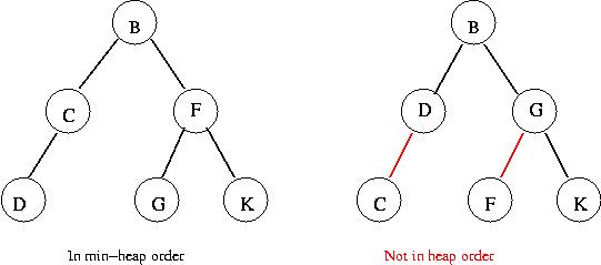
First, some definitions:
- A tree is in max-heap-order if every node is larger
than its children.
(That is, a node's key is larger than the keys in its child nodes).
- A tree is in min-heap-order if every node is smaller
than its children.
Example:
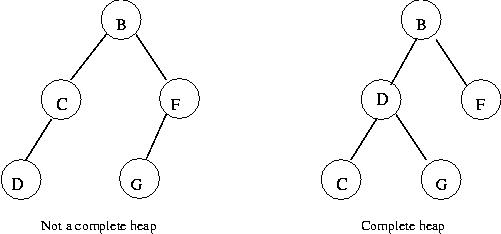
- A binary tree in heap order is called a binary heap
- A complete binary heap is a binary heap in which,
on the lowest level (furthest from the root), the only node with
no right sibling is the rightmost node.
Example:
Key ideas about binary heaps:
- The smallest (largest) element is always at the root in a min
(max) heap.
- The root can be extracted to leave behind a heap
in time O(log(n)).
- Using a min-heap for sorting:
- Build a heap in time O(n).
- Extract successive roots, re-adjusting the heap each time.
- Total time: O(n log(n)).
- Complete binary heaps can be efficiently represented using arrays.
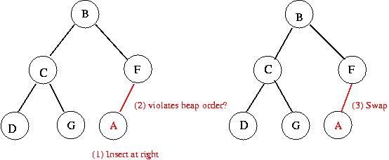
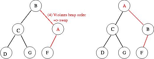
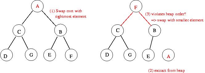
Insertion example:
Extracting min:
Implementing a binary min-heap:
- Store successive levels sequentially in an array.
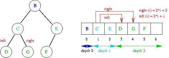
- Given an index into the array, the indices of the
parent, left and right child can be computed:
- Parent(i) = (i-1)/2.
- Left(i) = 2i+1.
- Right(i) = 2i+2.
In-Class Exercise 2.8:
- Show the status of the heap after the maximal element has
been extracted from this max-heap:
- Show the contents of the array representation of the heap.
- A complete binary tree is one in which all the leaves
are at the same depth. What is the number of nodes in a complete
binary tree of depth n? Show how to use the appropriate summation
formula from Module 1 to compute this number.
Pseudocode:
Key methods: minHeapify, buildMinHeap, extractMin:
- minHeapify:
Given an index, restore heap-order in the subtree at that
index if violated.
Algorithm: minHeapify (data, i)
Input:  heap, index into heap
1.  left = left (i);
2.  right = right (i);
3.  if (left < currentHeapSize) and (data[left] < data[i])
4.    smallest = left;
5.  else
6.    smallest = i;
7.  endif
8.  if (right < currentHeapSize) and (data[right] < data[smallest])
9.    smallest = right;
10. endif
11. if (smallest != i)
12.   swap (data, i, smallest);
13.   minHeapify (data, smallest);
14. endif
Output: subtree at i in min-heap-order
- buildMinHeap: build a heap from unsorted data
Algorithm: buildMinHeap (data)
Input:  data array
1. currentHeapSize = length of data;
   // Find the index from which the lowest level starts:
2. startOfLeaves = findStartOfLeaves (currentHeapSize);
3. for i=startOfLeaves-1 downto 0
4.      minHeapify (data, i);
5. endfor
Output:  a min-order heap constructed from the data.
- extractMin: remove the root (min) and restore heap-order
Algorithm: extractMin (data)
Input:  heap
    // Min element is in data[0].
1.  minValue = data[0];
    // Swap last element into root:
2.  data[0] = data[currentHeapSize-1];
    // Reduce heap size:
3.  currentHeapSize--;
    // Restore heap-order
4.  minHeapify (data, 0);
5.  return minValue;
Output:  minimum value
Sorting:
- First, build a min-heap from the data.
- Then, extract the min element one by one.
Example:
In-Class Exercise 2.9:
Draw the heap at each step in the above example.
Analysis:
- A complete binary tree with n nodes has maximum depth
log2(n):
- Start from the root and walk towards a lowest-level leaf.
- Each step down reduces the number-of-nodes in the current
subtree by at least half.
- The maximum depth of a heap with n nodes is
log2(n) = O(log (n)).
- Each buildHeap adjustment requires O(log(n)) effort
=> at most O(n log(n) to build the heap.
- Each extractMin requires O(log(n)) of work.
- For sorting, we extract n times.
=> O(n log(n)) sorting time overall.
- Space: O(n) extra space to extract the min's.
- Note: a more careful analysis of buildHeap shows
that it requires O(n) time.
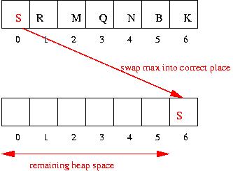
Sorting using a max-heap:
- It is possible to avoid the O(n) space by using a max-heap.
- Each time the max is extracted, it is placed in its correct
sort position.
- Key idea: once the max is extracted, its correct position is
not needed by the heap.
Maxheap example:
Building max heap: heapifying data[6] = I

 F A A E J K I C G D     P=6 L=13 R=14   Parent is smallest (=> no swap)
             ^
Building max heap: heapifying data[5] = K

 F A A E J K I C G D     P=5 L=11 R=12   Parent is smallest (=> no swap)
           ^
Building max heap: heapifying data[4] = J

 F A A E J K I C G D     P=4 L=9 R=10   Parent is smallest (=> no swap)
         ^         ^
Building max heap: heapifying data[3] = E

 F A A E J K I C G D     P=3 L=7 R=8   Right is smallest (=> swap right with root)
       ^       ^ ^

 F A A G J K I C E D     P=8 L=17 R=18   Parent is smallest (=> no swap)
                 ^
Building max heap: heapifying data[2] = A

 F A A G J K I C E D     P=2 L=5 R=6   Left is smallest (=> swap left with root)
     ^     ^ ^

 F A K G J A I C E D     P=5 L=11 R=12   Parent is smallest (=> no swap)
           ^
Building max heap: heapifying data[1] = A

 F A K G J A I C E D     P=1 L=3 R=4   Right is smallest (=> swap right with root)
   ^   ^ ^

 F J K G A A I C E D     P=4 L=9 R=10   Left is smallest (=> swap left with root)
         ^         ^

 F J K G D A I C E A     P=9 L=19 R=20   Parent is smallest (=> no swap)
                   ^
Building max heap: heapifying data[0] = F

 F J K G D A I C E A     P=0 L=1 R=2   Right is smallest (=> swap right with root)
 ^ ^ ^

 K J F G D A I C E A     P=2 L=5 R=6   Right is smallest (=> swap right with root)
     ^     ^ ^

 K J I G D A F C E A     P=6 L=13 R=14   Parent is smallest (=> no swap)
             ^

Heap construction complete


Heapifying after swapping max = K

 A J I G D A F C E K     P=0 L=1 R=2   Left is smallest (=> swap left with root)
 ^ ^ ^             |

 J A I G D A F C E K     P=1 L=3 R=4   Left is smallest (=> swap left with root)
   ^   ^ ^         |

 J G I A D A F C E K     P=3 L=7 R=8   Right is smallest (=> swap right with root)
       ^       ^ ^ |

 J G I E D A F C A K     P=8 L=17 R=18   Parent is smallest (=> no swap)
                 ^ |
Heapifying after swapping max = J

 A G I E D A F C J K     P=0 L=1 R=2   Right is smallest (=> swap right with root)
 ^ ^ ^           |

 I G A E D A F C J K     P=2 L=5 R=6   Right is smallest (=> swap right with root)
     ^     ^ ^   |

 I G F E D A A C J K     P=6 L=13 R=14   Parent is smallest (=> no swap)
             ^   |
Heapifying after swapping max = I

 C G F E D A A I J K     P=0 L=1 R=2   Left is smallest (=> swap left with root)
 ^ ^ ^         |

 G C F E D A A I J K     P=1 L=3 R=4   Left is smallest (=> swap left with root)
   ^   ^ ^     |

 G E F C D A A I J K     P=3 L=7 R=8   Parent is smallest (=> no swap)
       ^       ^ ^
Heapifying after swapping max = G

 A E F C D A G I J K     P=0 L=1 R=2   Right is smallest (=> swap right with root)
 ^ ^ ^       |

 F E A C D A G I J K     P=2 L=5 R=6   Parent is smallest (=> no swap)
     ^     ^ ^
Heapifying after swapping max = F

 A E A C D F G I J K     P=0 L=1 R=2   Left is smallest (=> swap left with root)
 ^ ^ ^     |

 E A A C D F G I J K     P=1 L=3 R=4   Right is smallest (=> swap right with root)
   ^   ^ ^ |

 E D A C A F G I J K     P=4 L=9 R=10   Parent is smallest (=> no swap)
         ^ |       ^
Heapifying after swapping max = E

 A D A C E F G I J K     P=0 L=1 R=2   Left is smallest (=> swap left with root)
 ^ ^ ^   |

 D A A C E F G I J K     P=1 L=3 R=4   Left is smallest (=> swap left with root)
   ^   ^ ^

 D C A A E F G I J K     P=3 L=7 R=8   Parent is smallest (=> no swap)
       ^ |     ^ ^
Heapifying after swapping max = D

 A C A D E F G I J K     P=0 L=1 R=2   Left is smallest (=> swap left with root)
 ^ ^ ^ |

 C A A D E F G I J K     P=1 L=3 R=4   Parent is smallest (=> no swap)
   ^   ^ ^
Heapifying after swapping max = C

 A A C D E F G I J K     P=0 L=1 R=2   Parent is smallest (=> no swap)
 ^ ^ ^
Heapifying after swapping max = A

 A A C D E F G I J K     P=0 L=1 R=2   Parent is smallest (=> no swap)
 ^ ^ ^
In-Class Exercise 2.10:
Apply the max-heap-sort to this data and show the array
contents:
A LowerBound
What is a lower bound?
- A lower bound for an algorithm: "this algorithm
takes at least f(n) time".
- A lower bound for a problem:
"this problem can't be solved faster than g(n) time".
- Lower bounds for problems are usually hard to prove.
Lower bound on sorting:
- Uses the comparison model: assumes that data can
only be compared.
(e.g., by using Java's Comparable interface).
- With this model: sorting cannot be done faster than O(n log(n)).
- Proof sketch:
BucketSort
In some applications, we can exploit knowledge about the data:
- Example: suppose we are sorting an array of small integers
that repeat frequently, e.g.,
7, 3, 1, 1, 1, 3, 5, 2, 5, 5, 6, 7, 8, 2, 2, 2, 1, ...
(no value larger than 10)
BucketSort for small-range integer data:
- Data is assumed to consist of integers in a small range.
- Key ideas:
How does this square with the lower bound?
- We have exploited inherent properties about the data.
- Too see why, consider this extreme case:
- Suppose we know the data contains all 1's and a single 0.
- Algorithm: write out 0, and the rest 1's.
- Time required: no sorting time, only output.
Note:
- Strings can be sorted by first hashing them into buckets.
- The above BucketSort for integers is sometimes called CountingSort.
Final Comments
- Sorting is one of the most-studied and most important problems in
Computer Science:
It has driven both theoretical research and practical solutions.
- Sorting has been studied in other contexts: parallel machines,
database systems, external sorting.