\( \newcommand{\blah}{blah-blah-blah} \newcommand{\eqb}[1]{\begin{eqnarray*}#1\end{eqnarray*}} \newcommand{\eqbn}[1]{\begin{eqnarray}#1\end{eqnarray}} \newcommand{\bb}[1]{\mathbf{#1}} \newcommand{\mat}[1]{\begin{bmatrix}#1\end{bmatrix}} \newcommand{\nchoose}[2]{\left(\begin{array}{c} #1 \\ #2 \end{array}\right)} \newcommand{\defn}{\stackrel{\vartriangle}{=}} \newcommand{\rvectwo}[2]{\left(\begin{array}{c} #1 \\ #2 \end{array}\right)} \newcommand{\rvecthree}[3]{\left(\begin{array}{r} #1 \\ #2\\ #3\end{array}\right)} \newcommand{\rvecdots}[3]{\left(\begin{array}{r} #1 \\ #2\\ \vdots\\ #3\end{array}\right)} \newcommand{\vectwo}[2]{\left[\begin{array}{r} #1\\#2\end{array}\right]} \newcommand{\vecthree}[3]{\left[\begin{array}{r} #1 \\ #2\\ #3\end{array}\right]} \newcommand{\vecdots}[3]{\left[\begin{array}{r} #1 \\ #2\\ \vdots\\ #3\end{array}\right]} \newcommand{\eql}{\;\; = \;\;} \newcommand{\eqt}{& \;\; = \;\;&} \newcommand{\dv}[2]{\frac{#1}{#2}} \newcommand{\half}{\frac{1}{2}} \newcommand{\mmod}{\!\!\! \mod} \newcommand{\ops}{\;\; #1 \;\;} \newcommand{\implies}{\Rightarrow\;\;\;\;\;\;\;\;\;\;\;\;} \newcommand{\prob}[1]{\mbox{Pr}\left[ #1 \right]} \newcommand{\expt}[1]{\mbox{E}\left[ #1 \right]} \newcommand{\probm}[1]{\mbox{Pr}\left[ \mbox{#1} \right]} \newcommand{\simm}[1]{\sim\mbox{#1}} \definecolor{dkblue}{RGB}{0,0,120} \definecolor{dkred}{RGB}{120,0,0} \definecolor{dkgreen}{RGB}{0,120,0} \)

Module 10: Optimization

10.1 Types of optimization problems

First, what is an optimization problem?

Typically, there is some objective
$\Rightarrow$ Maximize or minimize some value.

There must also be variables whose values we can choose
$\Rightarrow$ The value depends on choices made for these variables.

Key concepts in optimization techniques vary according to the type of optimization problem.
$\Rightarrow$ It's very rare for a principle to work across different types.

Broadly, one may categorize as follows:

Discrete optimization problems
$\Rightarrow$ Also called combinatorial optimization problems.
Continuous optimization problems
$\Rightarrow$ This has many sub-categories: linear, non-linear, quadratic etc.
Stochastic optimization problems:
$\Rightarrow$ Where there is some element of randomness.

Discrete optimization:

Example: the Traveling Salesman Problem (TSP).
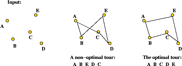
- Input: $n$ points on the plane.
- Objective: find a tour of minimum length.
A given instance has a finite (possibly large) number of candidate solutions.

Exercise 1: How many candidate tours can one construct for an $n$-point TSP problem?
Note: the problem is inherently discrete
- The solution is a finite set of edges.
- The set of candidate solutions is finite.
Algorithms for discrete problems do their search for solutions in a discrete space.

Continuous optimization:

In contrast, consider this problem:
minimize $f(x) = 5 + (x-4.71)^2$
In other words, find that value of $x$ where $f(x)$ is smallest.
The set of candidate solutions?
$\Rightarrow$ uncountably infinite (the real line)
Algorithms for these problems search a continuous space.
This example had only one variable: $x$.
In general, continuous optimization problems will have more than one variable
e.g., minimize $f(x,y,z) = 5 + (x-4.71)^2 + \frac{1}{(3y-z)} + \sin(xy)$
Jargon: the function to be optimized is called the objective function.

Function vs. parameter (or variable) optimization:

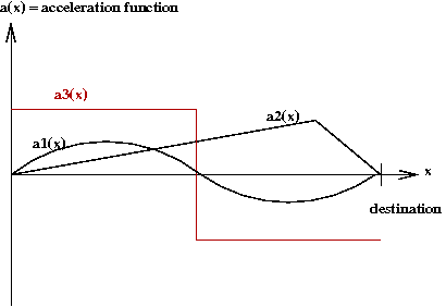
Recall the car acceleration problem from Module 1:
- Goal: Find that acceleration function to minimize travel time.
  Here, function $a_3(x)$ turns out to be better than functions $a_1(x)$ or $a_2(x)$.
Similarly, recall the two-segment incline problem from Module 3:
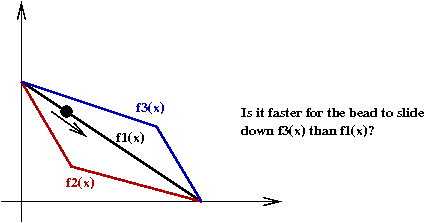
- The goal was to see which two segments result in the bead sliding down soonest.
- It turns out that $f_2(x)$ is better than the other two.
In both examples above, the goal is to find the best function.
However in problems like
e.g., minimize $f(x,y,z) = 5 + (x-4.71)^2 + \frac{1}{(3y-z)} + \sin(xy)$
We are given a function, and need to find the best values for its arguments (variables).
$\Rightarrow$ This is called parameter optimization.

Categories of continuous (parameter) optimization problems:

Constrained vs. unconstrained:
- Consider the example:
  minimize $f(x,y) = 5 + (x-4.71)^2 + 2y^3$
  such that $x + y = 5$.
- This is an example of a problem with constraints (on the variables).
Linear vs. non-linear objective function
- Non-linear example: $f(x,y) = 5 + (x-4.71)^2 + 2y^3$.
- Linear example: $f(x,y) = 5x + 7y$.
Linear vs. non-linear constraints:
- Linear constraints example:
  minimize $f(x,y) = 5 + (x-4.71)^2 + 2y^3$
  such that $x + y = 5$.
- Non-linear constraints example:
  minimize $f(x,y) = 5 + (x-4.71)^2 + 2y^3$
  such that $(x + y)^2 = 5$.
Note: it's the variables that are constrained.
Combinations of these lead to the important categories:
- Linear objective, unconstrained variables: this is a trivial problem.
  
  Exercise 2: Why is this true? What is the minimum (unconstrained) value of $f(x,y) = 3x + 4y$?
- Linear objective, linear constraints: one of the most important, and successful types of problems.
- Nonlinear, unconstrained: many kinds are solvable with iterative algorithms.
- Nonlinear, constrained: the hardest type of problem to solve
  $\Rightarrow$ Different techniques for sub-categories (e.g. linear constraints).

In this module:

We'll focus on nonlinear (mostly unconstrained) problems.
Mostly, we'll assume we have a function to minimize (as opposed to maximize).
Maximizing $f(x)$ is the same as minimizing $-f(x)$ (its reflection about the x-axis).
Notation:
- $f(x)$ denotes the objective function we wish to minimize.
- Let $x^*$ be the $x$-value that minimizes $f(x)$
  $\Rightarrow$ i.e., $f(x^*) ≤ f(x)$ for any other $x$.
Also, instead of using $x,y,z$ for multiple variables, we'll generally prefer $x_1,x_2,x_3$ etc.
So, for example, the function $f(x,y)=3x+4y$ in the above exercise would be written as $$ f(x_1,x_2) \eql 3x_1 + 4x_2 $$

10.2 What we learned in calculus

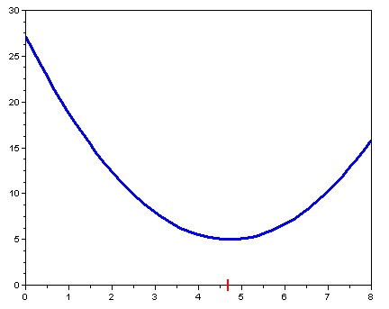
Let's go back to our example:

Consider the problem
minimize $f(x) = 5 + (x-4.71)^2$

In calculus, we learned to set $f'(x)=0$:
$f'(x)=0$
$\Rightarrow$ $f'(x) = 2(x-4.71) = 0$
$\Rightarrow$ $x = 4.71$

This approach relies on successfully solving two sub-problems:

Problem 1: calculating the derivative $f'(x)$.
$\Rightarrow$ i.e., finding an analytical formula for $f'(x)$. (such as $f'(x) = 2(x-4.71)$.
Problem 2: solving $f'(x)=0$.

In some real-world problems, it's hard to directly calculate $f'(x)$.

In most real-world problems, it's very difficult to solve (by hand) $f'(x)=0$.

Example: $f(x) = \sin(x) - x^2$

The first part is easy: $f'(x) = \cos(x) - 2x$.
The second part is very difficult: solving $\cos(x)-2x=0$.

However, it's fairly easy to write an algorithm to search for the optimal solution.
$\Rightarrow$ the focus of this module.

Exercise 3: Go back to your calc book and find an example of a "hard to differentiate" function.

Exercise 4: What's an example of a function that's continuous but not differentiable? Consider the (weird) function $f(x)$ where $f(x)=1$ if $x$ is rational and $f(x)=0$ otherwise. Is this continuous? Differentiable?

Exercise 5: Consider the function $$ f(x) \eql \frac{x}{\mu_1-\lambda x} + \frac{1-x}{\mu_2-\lambda(1-x)} $$
Compute the derivative $f'(x)$. Can you solve $f'(x)=0$?

One other important point from our calc course:

Merely solving $f'(x) = 0$ did not tell us whether this minimized or maximized $f$
$\Rightarrow$ We needed something else.
One way to tell: plot $f(x)$ and see where the gradient is zero.
A better way: evaluate the second derivative at the optimum.
negative 2nd derivative $\Rightarrow$ minimum.

10.3 Simple bracketing search

Key ideas:

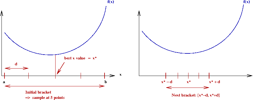
First, find a large enough initial range (bracket), $[a,b]$.

Pick values for the algorithm parameters
$M$ = number of intervals.
$N$ = number of iterations.

Then, divide the bracket into $M$ intervals
$\Rightarrow$ Let $\delta = \frac{b-a}{M}$.

Evaluate $f(x)$ at every interval boundary.

Pick the best such $x$
$\Rightarrow$ Call this $x^*$.

Set the new bracket to be $[x-\delta,x+\delta]$.

Repeat (for a total of $N$ times).

Pseudocode:

     Algorithm: bracketSearch (a, b)
     Input: the initial range [a,b]
     1.    for i=1 to N                 
     2.        δ = (b-a) / M            // Divide current bracket.
     3.        x* = a
     4.        bestf = f(x*)
     5.        for x=a to b step δ      // Search for best x in current bracket
     6.            f = f(x)
     7.            if f < bestf
     8.                bestf = f
     9.                x* = x
     10.           endif
     11.       endfor
     12.       a = x* - δ               // Shrink bracket.
     13.       b = x* + δ
     14.   endfor
     15.   return x*

Exercise 6: Download and execute BracketSearch.java.

What is the running time in terms of $M$ and $N$?
If we keep $MN$ constant (e.g., $MN=24$), what values of $M$ and $N$ produce best results?

Exercise 7: Draw an example of a function for which bracket-search fails miserably, that is, the true minimum is much lower than what's found by bracket search even for large $M$ and $N$.

How does one evaluate such algorithms?

In the above case, the actual computation inside the innermost loop was simple
$\Rightarrow$ Computing $f(x)$ takes constant time.
However, in many real-world examples
$\Rightarrow$ Computing $f(x)$ can take a lot of time.
Example: $f(x)$ may be the result of solving a differential equation
$\Rightarrow$ Computing $f(x)$ itself needs multiple iterations.
Thus, one would like to reduce the number of function evaluations.

Exercise 8: What is the number of function evaluations in terms of $M$ and $N$ for the bracket-search algorithm?

Can bracket search work for multivariate functions such as $f(x,y) = 2x+3y^2$?

Yes, one simply divides every dimension at each step
$\Rightarrow$ The brackets become "cells"

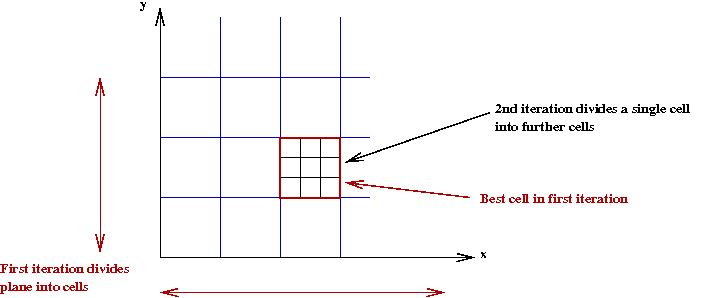
For example, in 2D (2 variables)

     Algorithm: bracketSearch (a₁, b₁, a₂, b₂)
     Input: the initial ranges for each dimension [a₁, b₁] and [a₂, b₂]
     1.    for i=1 to N                 
               // The ranges could be different in each dimension.
     2.        δ₁ = (b₁ - a₁) / M
     3.        δ₂ = (b₂ - a₂) / M
     4.        x₁* = a₁,  x₂* = a₂
     5.        bestf = f(x₁*, x₂*)
     6.        for x₁=a₁ to b₁ step  δ₁     
     7.            for x₂=a₂ to b₂ step  δ₂
     8.                f = f(x₁,x₂)
     9.                if f < bestf
     8.                    bestf = f
     9.                    x₁* = x₁,  x₂* = x₂
     10.               endif
     11.           endfor
     12.       endfor
               // Shrink cell.
     13.       a₁ = x₁* -  δ₁,   b₁ = x₁* + δ₁
     14.       a₂ = x₂* -  δ₂,   b₂ = x₂* + δ₂
     15.   endfor
     16.   return x₁*, x₂*

Notice that we've used the notation $(x_1,x_2)$ instead of $(x,y)$.
$\Rightarrow$ For an n-dimensional space we'd use $(x_1,x_2, ..., x_n)$ to represent a particular point.

Exercise 9: What is the number of function evaluations in terms of $M$ and $N$ for the 2D bracket-search algorithm? How does this generalize to $n$ dimensions?

Exercise 10: Add code to MultiBracketSearch.java to find the minimum of $f(x_1,x_2)=(x_1-4.71)^2 + (x_2-3.2)^2 + 2(x_1-4.71)^2(x_2-3.2)^2$.

When to stop?

We have fixed the number of iterations at $N$.
We could, instead, stop when some desired accuracy is achieved.
Let's try the following:
- Let $f_k$ be the best value after $k$ iterations.
- We will compare $f_k$ and $f_{k-1}$.
  If $|f_k - f_{k-1}| \lt \epsilon$, then stop.
- Here, $\epsilon$ is some suitably small number.

In pseudocode:

     Algorithm: bracketSearch (a, b)
     Input: the initial range [a,b]
     1.    bestf = some-large-value
     2.    prevBestf = bestf + 2ε         // So that we enter the loop.
     3.    while |bestf - prevBestf| > ε
     4.        δ = (b-a) / M              
     5.        x* = a
     6.        prevBestf = bestf
     7.        bestf = f(x*)
     8.        for x=a to b step δ
     9.            f = f(x)
     10.           if f < bestf
     11.               bestf = f
     12.               x* = x
     13.           endif
     14.       endfor
     15.       a = x* - δ               
     16.       b = x* + δ
     17.       N = N + 1                  // Track N for printing/evaluation
     18.   endfor
           // Print N if desired.
     19.   return x*

How do we choose $\epsilon$?
- If, in our problem, $f$ values happen to be very large (e.g, $10^6$),
  $\Rightarrow$ $\epsilon=0.1$ may be unnecessarily small.
- If, on the other hand, $f$ values happen to be very small (e.g, $10^{-6}$),
  $\Rightarrow$ $\epsilon=0.1$ may be too large.
  $\Rightarrow$ No optimization occurs.
A better solution:
Stop when $$ \left| \frac{f_k - f_{k-1}}{f_{k-1}}\right| \; \lt \; \epsilon $$
$\Rightarrow$ Thus, if the proportional change is very small, stop.

Exercise 11: Modify BracketSearch2.java to use the proportional-difference stopping condition.

10.4 Golden ratio search

First, an important observation:

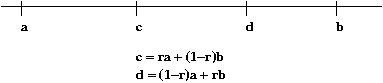
Suppose $a \lt b$ are two real numbers.
$\Rightarrow$ e.g., they represent an interval $[a,b]$.

Next, let $r$ be a number strictly between $0$ and $1$.
$\Rightarrow$ i.e., $0 \lt r \lt 1$.

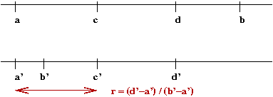
Now consider the numbers $c = ra + (1-r)b$, and $d = (1-r)a + rb$.

Then, it is true that $a \lt c \lt b$
$\Rightarrow$ That is, $c$ is between $a$ and $b$.

Similarly, $a \lt d \lt b$

Intuition:

Pick $r=0.3$ and $a=4, b=9$.
Then, $c = 0.3*4 + 0.7*9$ = some weighted average of $4$ and $9$
$\Rightarrow$ weighted average must be between $4$ and $9$.

Exercise 12: Prove this result.

Next, let's look at the ideas in ratio search (before we tackle golden-ratio search):

Recall that, in bracket-search, we fixed the number of intervals $M$.
In ratio search, we will use $M=1$ but adjust the ends.
Start with some interval $[a,b]$.
Compute the ends of a smaller interval contained within:
At each step, shrink the interval to either $[a,d]$ or $[c,b]$.
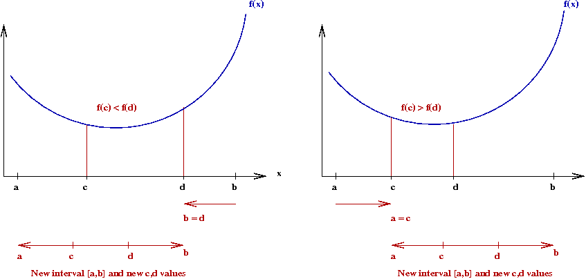
- If $f(c) \leq f(d)$, set $b = d$.
- If $f(c) \gt f(d)$, set $a = c$.
Then, repeat until interval is small enough to stop.
Why does this work?
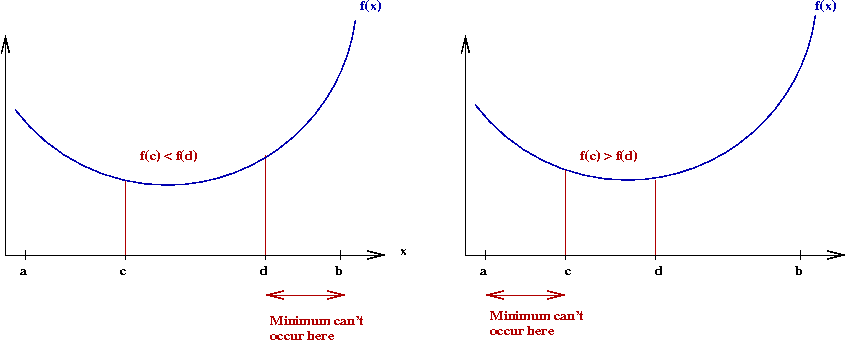
- First, we assume the function is unimodal
  $\Rightarrow$ $f(x)$ decreases from $a$ to the optimal $x$, and increases after that.
- If $f(c) \leq f(d)$, then the minimum cannot occur to the right of $d$.
  $\Rightarrow$ We can shrink the interval on the right.
- Same reasoning for the left side.
After shrinking the interval, we again compute two interior points and repeat.

Golden-ratio search:

Recall what happens after shrinking an interval:
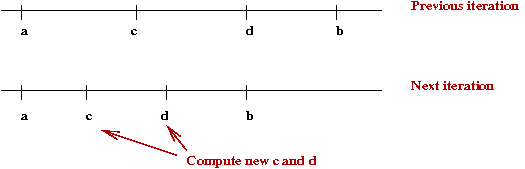
- We re-compute new $c$ and $d$ values after shrinking.
Instead, suppose we could re-use one of the previous values:
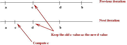
How do we arrange for this to happen? Is there a value of $r$ that will make this happen?
First, observe

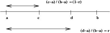
Thus $$ \frac{(c-a)}{(b-a)} \eql (1-r) $$ Or $(1-r)$ = ratio of the distance $c-a$ to the whole interval
Similarly, $$ \frac{(d-a)}{(b-a)} \eql (1-r) $$

Exercise 13: Prove this result.
Next, consider two iterations:

The ratio $$\eqb{ r \eqt \frac{d' - a'}{b' - a'} \\ \eqt \frac{d' - a'}{d - a} \\ \eqt \frac{c - a}{d - a} \\ \eqt \frac{(1-r)(b - a)}{r(b - a)} \\ \eqt \frac{(1-r)}{r} \\ }$$
Simplifying, we get $r^2 + r - 1 = 0$.
This famous quadratic has the solution $r = 0.618...$ (approx.)
$\Rightarrow$ called the golden ratio.

Pseudocode:

     Algorithm: goldenRatioSearch (a, b)
     Input: the initial range [a,b]
     1.    Pick c and d so that |(c-d)/d| > ε
     2.    while |(c-d)/d| > ε
     3.        if fc ≤ fd
     4.            b = d                  // Shrink from right side.
     5.            d = c                  // Re-use old c, f(c).
     6.            fd = fc
     7.            c = ra + (1-r)b        // Compute new c, f(c).
     8.            fc = f(c)
     9.        else
     10.           a = c                  // Shrink from left side.
     11.           c = d                  // Re-use old d, f(d).
     12.           fc = fd  
     13.           d = (1-r)a + rb        // Compute new d, f(d).
     14.           fd = f(d)
     15.       endif
     16.   endwhile
     17.   return (c+d)/2

Exercise 14: Describe what could go wrong if we replaced the while-condition with

     2.    while |(fc-fd)/fd| > ε

How would you address this problem?

Exercise 15: Implement golden-ratio search in this template: GoldenRatio.java.

10.5 Gradient descent

Let's start by understanding what gradient means:

Consider a (single-dimensional) function $f(x)$:

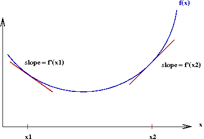
Let $f'(x)$ denote the derivative of $f(x)$.
The gradient at a point $x$ is the value of $f'(x)$.
$\Rightarrow$ Graphically, the slope of the tangent to the curve at $x$.

Observe the following:

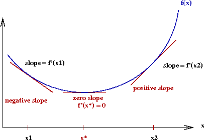
To the left of the optimal value $x^*$, the gradient is negative.
To the right, it's positive.

We seek an iterative algorithm of the form

     while not over
         if gradient < 0
             move rightwards
         else if gradient > 0
             move leftwards
         else
             stop               // gradient = 0 (unlikely in practice, of course)
         endif
     endwhile

The gradient descent algorithm is exactly this idea:

     while not over
         x = x - α f'(x)
     endwhile

Here, we add a scaling factor $\alpha$ in case $f'(x)$ values are of a different order-of-magnitude:

Why we need $\alpha$

For example, it could be that $x=0.1, x^*=0$ and $f(0.1)=1000$.
Then one iterative step without $\alpha$ would produce $x = 0.1 - 1000 = -999.9$
$\Rightarrow$ Which would be way out of bounds.
For such a problem, we'd use $\alpha = 0.0001$ so that
$x = 0.1 - 0.0001*1000 = 0.09$

The algorithm parameter $\alpha$ is sometimes called the stepsize.

In pseudocode:

     Algorithm: gradientDescent (a, b)
     Input: the range [a,b]
     1.    x = a                      // Alternatively, x = b.
     2.    while |f'(x)| > ε
     3.        x = x - α f'(x)        // Note: f'() is evaluated at current value of x (before changing x).
     4.    endwhile
     5.    return x

Stopping conditions:

The obvious stopping condition is to see whether $f'(x)$ is close enough to zero.
However, this may not always work:
$\Rightarrow$ If $\alpha$ is too small, the gradient may never get close enough.
Thus, it may help to also evaluate the actual proportional change in $x$, that is, $$ \left| \frac{\mbox{prevX-x}}{\mbox{prevX}} \right| $$

Exercise 16: Download and execute GradientDemo.java.

How many iterations does it take to get close to the optimum?
What is the effect of using a small $\alpha$ (e.g, $\alpha=0.001$)?
In the method nextStep(), print out the current value of $x$, and the value of $xf'(x)$ before the update.
Set $\alpha=1$. Explain what you observe.
What happens when $\alpha=10$?

Picking the right stepsize:

Clearly, the performance of gradient descent is sensitive to the choice of the stepsize $\alpha$.
- If $\alpha$ is too small
  $\Rightarrow$ It can take too long to converge.
- If $\alpha$ is too large
  $\Rightarrow$ It can diverge or oscillate, and never converge.
One rule of thumb: the term $\alpha f'(x)$ should be an order-of-magnitude less than $x$.
$\Rightarrow$ This way, the changes in $x$ are small relative to $x$.
Another idea: try different $\alpha$ values in each iteration:
- Start with a small $\alpha$.
- Gradually increase until it "does something bad".
- What is "bad"?
  $\Rightarrow$ Causes an increase in $f(x)$ value.
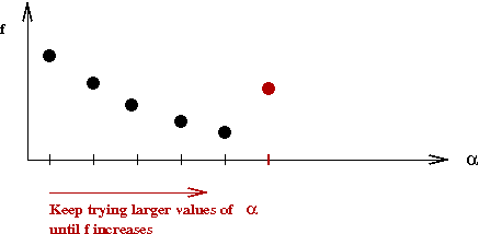
- This idea is called line-search
  $\Rightarrow$ Because we're searching along the (single) dimension of $\alpha$.

At first, it may seem that one could merely try increasing $α$:

  Algorithm: gradientDescentLineSearch (a, b)
  Input: the range [a,b]
  1.    x = a                      
  2.    while |f'(x)| > ε
  3.        α_trial = α_small                  // α_small is the first value to try.
  4.        do                             // Search for the right alpha.
  5.            α = α_trial
  6.            α_trial = α + δ_α
  7.            f = f(x - αf'(x))
  8.            f_trial = f(x - α_trialf'(x))
  9.        while f_trial < f                // Keep increasing stepsize until you get an increase in f
  10.       x = x - α f'(x)  
  11.   endwhile
  12.   return x

However, this approach has two problems:
- It is highly dependent on the choice of $\delta_{\alpha}$.
- What if the true best value is extremely small (smaller than $\delta_{\alpha}$)?
  $\Rightarrow$ We'd overlook it because it falls between [α_small, α_small+δ_α]

The better way is to realize that we can use bracketing search, which automatically adjusts to the "scale" by shrinking intervals:

  Algorithm: gradientDescentLineSearch (a, b)
  Input: the range [a,b]
  1.    x = a                      
  2.    Pick α_small                   // Left end of  α interval
  3.    Pick α_big                     // Right end of  α interval
  4.    while |f'(x)| > ε
            // Define the function g(α) = f(x - αf'(x)) in the interval [α_small, α_big]
  5.        α* = bracketSearch (g, α_small, α_big)
  6.        x = x - α* f'(x)  
  7.    endwhile
  8.    return x

Let's now turn to an important concept that pervades all of optimization: local vs. global minima.

Exercise 17: Download GradientDemo2.java and examine the function being optimized.

Fill in the code for computing the derivative.

Try an initial value of $x$ at $1.8$. Does it converge?

Next, try an initial value of $x$ at $5.8$. What is the gradient at the point of convergence?

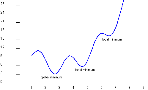
About local vs. global optima:

Just because the gradient is zero, doesn't mean we've found the optimum.
A function can have several different local minima, as we've seen.

Exercise 18: Can a function have several global minima?
The gradient $f'(x)$ at a point $x$ merely describes the behavior of the function $f$ near that point.
A gradient-descent algorithm will find a local minimum
$\Rightarrow$ There's no guarantee that it'll find the global minimum.
In general, apart from searching the whole space of solutions, there's no method that guarantees finding a global minimum.
Thus, finding a local minimum is considered a high-enough standard for an algorithm.

What if we cannot compute the gradient?

For some functions, a formula for the gradient may be difficult to obtain.
However, it's easy to approximate the gradient:
- Pick some small value $s$.
- Compute
  $\Rightarrow$ $f'_{approx}(x) = \frac{f(x+s) - f(x)}{s}$

In pseudocode:

     Algorithm: gradientDescentApprox (a, b)
     Input: the range [a,b]
     1.    x = a                      
     2.    f'_approx = 2ε
     3.    while |f'_approx| > ε
     4.        f'_approx = (f(x+s) - f(x)) / s       // s is an algorithm parameter.
     5.        x = x - α f'_approx       
     6.    endwhile
     7.    return x

Exercise 19: Add code to GradientDemo3.java to implement approximate gradients. Use $s=0.01$. Explain what could go wrong if $s$ is too large.

Theoretical issues:

The big questions:
Does the gradient-descent algorithm always converge to a local minimum?
Under what conditions does the algorithm converge?
Theoreticians usually describe such iterative algorithms using this notation: $$ x^{(n+1)} \eql x^{(n)} - \alpha f'(x^{(n)}) $$
Here, $x^{(n)}$ is the $n$-th iterate.
The convergence question:
- Let $S^*$ be the set of local minima.
- Question 1: Does the sequence $x^{(n)}$ have a limit?
- Question 2: If so, is the limit in $S^*$?
It can be shown that:
- If the function $f$ is "smooth" (twice-differentiable);
- and if $\alpha$ is small enough.
Then, $x^{(n)} \to x^*$, where $x^*$ is some point in $S^*$.
In the case that we use approximate gradients, we need an additional condition:
- Recall that our approximate gradient was computed as:
  $\Rightarrow$ $f'_{approx}(x) = \frac{f(x+s) - f(x)}{s}$
- We'll write the algorithm as
```
         while |f'_approx| > ε
             f'_approx = (f(x+s) - f(x)) / s 
             x = x - α f'_approx       
             n = n + 1
         endwhile
     
```
- Because $s$ is never exactly zero, it can never converge to the true minimum.
- To solve this problem, we need to gradually decrease $s$ as we iterate.
  $\Rightarrow$ i.e., let $s \to 0$ as $n$ increases.
- One way to do this:
```
         while |f'_approx| > ε
             s_n = s / n
             f'_approx = (f(x+s_n) - f(x)) / s_n
             x = x - α f'_approx       
             n = n + 1
         endwhile
     
```

10.6 Gradient descent in multiple dimensions

Recall the intuition behind the gradient-descent algorithm in one dimension:

First, what does gradient mean? Roughly, the change in $f$ with respect to increasing $x$: $$ f'(x) \; \approx \; \frac{f(x+s) - f(x)}{s} $$ (for small $s$)

We use the gradient to take a "step" in the direction towards the minimum:

         x = x - α f'(x)

Here, the "step" has two meanings:

A direction
$\Rightarrow$ determined by the sign of $f'(x)$.
A magnitude
$\Rightarrow$ determined by the magnitude of $f'(x)$.

The same idea works in multiple dimensions, provided we define "gradient" correctly.

Gradients for multivariable functions:

Let's first understand what we need:

We want an iterative algorithm for two variables.

What would this look like?

         while not over
            x₁ = x₁ - (some gradient)
            x₂ = x₂ - (some gradient)
         endwhile

Example: consider the function $f(x_1,x_2)=(x_1-4.71)^2 + (x_2-3.2)^2 + 2(x_1-4.71)^2(x_2-3.2)^2$.
$\Rightarrow$ This is a function of two variables, $x_1$ and $x_1$.
One option for defining the gradient would be $$ f'(x_1,x_2) \eql \frac{f(x_1+s,x_2+s) - f(x_1,x_2)}{s} $$ (for small $s$)
- This results in a single number.
- This means that the iteration would look like
```
         while not over
            x₁ = x₁ - α f'(x₁,x₂)
            x₂ = x₂ - α f'(x₁,x₂)
         endwhile
         
```
- Thus, the two variables would change by the same amount in the same direction.
Exercise 20: Explain why this won't work. Think up a function for which it won't work.
Instead, we need to compute gradients independently for each of the two variables: $$\eqb{ f'_1 \eqt \frac{f(x_1+s,x_2) - f(x_1,x_2)}{s} \\ f'_2 \eqt \frac{f(x_1,x_2+s) - f(x_1,x_2)}{s} }$$ (for small $s$)
These kinds of derivatives are called a partial derivatives.
$\Rightarrow$ There are two partial derivatives above, one for each variable.

In this case, our gradient descent algorithm looks like:

         while not over
            x₁ = x₁ - α f'₁(x₁,x₂)
            x₂ = x₂ - α f'₂(x₁,x₂)
         endwhile

Exercise 21: Compute by hand the partial derivatives of $f(x_1,x_2)=(x_1-4.71)^2 + (x_2-3.2)^2 + 2(x_1-4.71)^2(x_2-3.2)^2$.

Exercise 22: Compute by hand the partial derivatives of $$ f(x_1,x_2) \eql \frac{x_1}{\mu_1-\lambda x_1} \; + \; \frac{x_2}{\mu_2-\lambda x_2} $$

A little more detail:

What about the stopping condition?
$\Rightarrow$ We should keep going as long as any one of the gradients is not close to zero.
Same stepsize for both variables?
- In many problems, a single stepsize will suffice.
- A line-search will likely result in different stepsizes.

At first glance, it may seem that the pseudocode could be written as:

     1.    while |f₁'(x₁,x₂)| > ε or |f₂'(x₁,x₂)| > ε
     2.        x₁ = x₁ - α f₁'(x₁,x₂)
     3.        x₂ = x₂ - α f₂'(x₁,x₂)
     4.    endwhile

While mathematically more elegant this, however, creates a small programming issue, as we'll see.

Instead, let's use this pseudocode:

     Algorithm: twoVariableGradientDescent (a₁, b₁, a₂, b₂)
     Input: the ranges [a₁, b₁] and [a₂, b₂]
     1.    x₁ = a₁, x₂ = a₂
     2.    f₁' = 2ε
     3.    f₂' = 2ε
     4.    while |f₁'| > ε or |f₂'| > ε
     5.        f₁' = f₁'(x₁,x₂)
     6.        f₂' = f₂'(x₁,x₂)
     7.        x₁ = x₁ - α f₁'
     8.        x₂ = x₂ - α f₂'
     9.    endwhile
     10.   return x₁,x₂

Exercise 23: What would go wrong if we interchanged lines 6 and 7 above?

Note: just like the unidimensional case, we could use approximate gradients.

Exercise 24: Add code to MultiGradient.java to compute the partial derivatives of the function $f(x_1,x_2)=(x_1-4.71)^2 + (x_2-3.2)^2 + 2(x_1-4.71)^2(x_2-3.2)^2$. Then execute to find the minimum. You might need to experiment with different values of $\alpha$.

10.7 Stochastic gradient descent and simulation optimization

Let's start with an application:

Recall the routing problem with two queues:

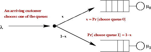
An arriving customer chooses queue 0 with $\probm{choose 0} = x$.
$\Rightarrow$ $\probm{choose 1} = 1-x$.

In the simulation,

         if uniform() < x
             choose 0
         else
             choose 1

Thus, one can consider $x$ to be a routing variable.

For a given routing probability $x$, there will be some average system time.

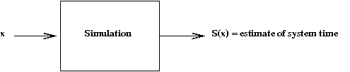
Here, for a particular value of $x$, we will get some estimate of the system time.
Let rv $S(x)$ denote the system time when using routing value $x$.

The goal: find that value $x$ that minimizes average system time $E[S(x)]$.

Exercise 25: Examine QueueControl.java and find the part of the code that chooses the queue. Try running the simulation with different values of $x$ to guess the minimum.

Let's try using gradient descent:

Recall the gradient-descent algorithm (for one variable):
```
         x = x - α f'(x)
      
```
How do we know what $f'(x)$ is?

One option: approximate it using finite differences

     while not over
         fxs = estimate system time with x+s       // Run the simulation with x+s
         fx  = estimate system time with x         // Run the simulation with x
         f' = (fxs - fx) / s                       // Compute finite difference.
         x = x - α f'                              // Apply gradient descent.
     endwhile

Exercise 26: Confirm that QueueOpt.java implements this approach. Run the algorithm - does it work? How many samples are used in each estimate?

The problem with noise:

Observe that we are not calculating the approximate-gradient but, rather, are estimating it.
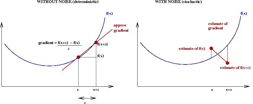
For any finite number of samples, an estimate will be off by some error.
Thus, the algorithm can "wander" all over $x$ space when using "noisy" estimates.
Fortunately, there are (interesting) ways around this problem.

Addressing the noise problem:

First, we'll identify how many samples are being used in each estimate.
- Recall that, in the example, we ran the simulation for 1000 departures.
- Obviously the more departures, the better the estimate.
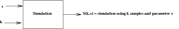
- Let $S(k,x)$ = estimate obtained using $k$ samples.
We will allow the number of such samples to vary by iteration.
Second, we'll allow the stepsize to vary by iteration.

Putting these ideas together, our iterative algorithm becomes

     while not over
         k = k_n                        // k = #samples to be used in iteration n
         fxs = S(k, x+s)               // Run the simulation with x+s
         fx  = S(k, x)                 // Run the simulation with x
         f' = (fxs - fx) / s           // Compute finite difference.
         α = α_n                        // Stepsize to be used in iteration n
         x = x - α f'                  // Apply gradient descent.
     endwhile

We could write this more mathematically as: $$ x^{(n+1)} \eql x^{(n)} - \alpha_n \frac{S(k_n,x^{(n)}+s) - S(k_n,x^{(n)})}{s} $$
What values should be used for $k_n$ and $\alpha_n$?
$\Rightarrow$ There are two approaches, stepsize-control and sampling-control
We'll look at each of these next.

Stepsize-control:

The key idea in stepsize control is to let the stepsize decrease gradually.
- Initially, we make possibly large noise-driven steps.
- Later, as we get closer to the optimum, the stepsizes get small.
One caveat: if the stepsize gets small too quickly, we may converge to some point away from the optimum.
Consider stepsizes that meet these conditions:
- $\alpha_n \to 0$.
- $\sum_n \alpha_n \to \infty$.
Thus, the stepsizes $\alpha_n$ decrease, but not too quickly.

Exercise 27: Give an example of such a sequence. (Hint: we saw one such example in Module 1). Also give an example of a sequence that does decrease quickly, that violates the second condition.
What about the numbers of samples $k_n$?
$\Rightarrow$ We'll pick a fixed number, e.g., $k_n=1000$?

Then, the algorithm can be written as follows:

  Algorithm: stepsizeControl 
       // Initialize x, other variables ... (not shown)

  1.   while not over
  2.       fxs = S(k, x+s)               // Run the simulation with x+s using k samples
  3.       fx  = S(k, x)                 // Run the simulation with x using k samples
  4.       f' = (fxs - fx) / s           // Compute finite difference.
  5.       α = α_n                        // stepsize to be used in iteration n
  6.       x = x - α f'                  // Apply gradient descent.
  7.       n = n + 1
  8.  endwhile
  9.  return x

The stepsize-control approach is sometimes called the Robbins-Munro algorithm.

Exercise 28: Modify StepsizeControl.java to use decreasing stepsizes. Does it work?

Sampling-control:

The other approach is to increase the number of samples:
- Initially, use fewer samples.
- Later, as we approach the optimum, use more samples.
For example, $k_n = n$

In this case, the algorithm can be written as:

  Algorithm: samplingControl 
       // Initialize x, other variables ... (not shown)

  1.  while not over
  2.       k = k_n                        // # samples for iteration n
  3.       fxs = S(k, x+s)               // Run the simulation with x+s using k samples
  4.       fx  = S(k, x)                 // Run the simulation with x using k samples
  5.       f' = (fxs - fx) / s           // Compute finite difference.
  6.       x = x - α f'                  // Note fixed stepsize.
  7.       n = n + 1
  8.  endwhile
  9.  return x

Finally, how do we know these methods worked for our routing example?

It turns out that one can analytically derive the system-time in terms of $x$: $$ f(x) \eql \frac{x}{\mu_1-\lambda x} \; + \; \frac{1-x}{\mu_2-\lambda(1-x)} $$
This can even be minimized analytically (see earlier exercise).
However, let's use our gradient-descent algorithm.

Exercise 29: Add code to QueueGradientDescent.java to find the minimum. Does this correspond with what you found when using the stepsize-control algorithm?

10.8 Summary

We have taken an in-depth look at single-variable unconstrained optimization:

Simple non-gradient methods: bracketing, golden-ratio search.

Gradient descent.

The difference between local and global minima.

Why gradient descent can get stuck in a local minima.

Stochastic version of gradient descent.

Multivariable version of gradient descent.

Related topics we haven't covered in non-linear optimization:

Ways to speed up gradient-descent
$\Rightarrow$ Using 2nd derivatives (e.g., Newton-Raphson method).
Constrained optimization
$\Rightarrow$ A big topic in itself.
Function optimization
$\Rightarrow$ Another big topic in itself.