\(
\newcommand{\blah}{blah-blah-blah}
\newcommand{\eqb}[1]{\begin{eqnarray*}#1\end{eqnarray*}}
\newcommand{\eqbn}[1]{\begin{eqnarray}#1\end{eqnarray}}
\newcommand{\bb}[1]{\mathbf{#1}}
\newcommand{\mat}[1]{\begin{bmatrix}#1\end{bmatrix}}
\newcommand{\nchoose}[2]{\left(\begin{array}{c} #1 \\ #2 \end{array}\right)}
\newcommand{\defn}{\stackrel{\vartriangle}{=}}
\newcommand{\rvectwo}[2]{\left(\begin{array}{c} #1 \\ #2 \end{array}\right)}
\newcommand{\rvecthree}[3]{\left(\begin{array}{r} #1 \\ #2\\ #3\end{array}\right)}
\newcommand{\rvecdots}[3]{\left(\begin{array}{r} #1 \\ #2\\ \vdots\\ #3\end{array}\right)}
\newcommand{\vectwo}[2]{\left[\begin{array}{r} #1\\#2\end{array}\right]}
\newcommand{\vecthree}[3]{\left[\begin{array}{r} #1 \\ #2\\ #3\end{array}\right]}
\newcommand{\vecdots}[3]{\left[\begin{array}{r} #1 \\ #2\\ \vdots\\ #3\end{array}\right]}
\newcommand{\eql}{\;\; = \;\;}
\newcommand{\dv}[2]{\frac{#1}{#2}}
\newcommand{\half}{\frac{1}{2}}
\newcommand{\mmod}{\!\!\! \mod}
\newcommand{\ops}{\;\; #1 \;\;}
\newcommand{\implies}{\Rightarrow\;\;\;\;\;\;\;\;\;\;\;\;}
\definecolor{dkblue}{RGB}{0,0,120}
\definecolor{dkred}{RGB}{120,0,0}
\definecolor{dkgreen}{RGB}{0,120,0}
\)
Module 1: Preliminaries
1.1 Integers vs. reals
First, integers:
- We usually include both positive and negative
integers
\(\mathbb{Z} = \{\ldots, -3, -2, -1, 0, 1, 2, 3, \dots\} \)
- Note: \( \mathbb{N} = \{1, 2, 3, \ldots\} \)
are the natural numbers.
- In many problems, we might only consider particular
(finite or infinite) subsets of \(\mathbb{Z}\)
- Some famous problems:
- (Solved) Fermat's Last Theorem: There are no integers
\(x,y,z\) such that \(x^n + y^n = z^n\)
for some integer \(n \geq 3\).
- (Unsolved) Goldbach's conjecture (1742): Every even
integer greater than 2 can be written as the sum of two primes.
- (Unsolved - Millenium Prize) Riemann Hypothesis: The real part of any
non-trivial zero of the Riemann zeta function is 1/2.
- (Unsolved) Polynomial-time algorithm for factorizing an integer.
An example of computing with integers: Euclid's GCD algorithm:
- For positive integers \(m\) and \(n\),
\(GCD(m,n) \defn \) the largest integer that divides
both \(m\) and \(n\).
- The symbol \(\defn\) means "is defined as".
- Example:
- 48 has divisors 1, 2, 3, 4, 6, 8, 12, 16, 24, 48.
- 32 has divisors 1, 2, 4, 8, 16, 32.
- Thus, GCD (32, 48) = 16.
- Algorithm 1:
- Factorize \(m\) and \(n\) separately.
- Search factors to find largest common factor.
- Analysis of Algorithm 1: factorization is hard.
⇒
No polynomial-time algorithm is known.
- Some observations:
- Suppose \(m \gt n\) and \(k\) divides both.
⇒
Then \(k\) divides \((m - n)\).
- In fact, as long as these numbers are positive,
\(k\) divides \((m - n), (m - 2n), (m - 3n) \ldots \)
- What is the smallest positive number in this list?
⇒
\(m \mmod n\)
- Thus, \(GCD (m, n)\) divides \(m \mmod n\).
- And because \(GCD (m, n)\) already divides \(n\),
it's among the common divisors of both \(n\) and \(m \mmod n\).
- Any of these common divisors of \(n\) and \(m \mmod n\)
must also divide \(m\), in particular, the largest one,
\(GCD (n, m \mmod n)\).
- Thus, \(GCD (m, n) \eql GCD (n, m \mmod n)\).
⇒
Divide and conquer!
Algorithm 2 (Euclid): (in Java)
     Algorithm: gcd (m, n)
     Input: integers m, n > 0

          // Check for bad input.
     1.   if n > m
     2.       return gcd (n,m)
     3.   endif

          // The algorithm.
     4.   if n = 0
     5.       return m;
     6.   else
     7.       return gcd (n, m mod n)
     8.   endif
- Analysis:
- Note that \(m \mmod n \lt n\).
- If \(n \leq \dv{m}{2}\), then \(m \mmod n \;\;\lt \;\; n \;\;\leq \;\; \dv{m}{2}\).
- If \(n \gt \dv{m}{2}\), then \(m \mmod n \eql m - n \;\;\leq\;\; \dv{m}{2}\).
- Thus, the larger number is reduced by \(\dv{1}{2}\) each time.
⇒
Thus, the running time is at most \(O(\log m)\).
A few more observations:
- Euclid's algorithm is recursive.
- The size of the problem is small:
⇒
We need \(O(\log m)\) bits to represent the numbers.
- The running time is linear in the size
of the problem.
As it turns out, these characteristics (recursion,
problem-size) are classically associated with discrete
algorithms.
⇒
Algorithms for continuous structures rarely have these properties.
Now let's look at real numbers:
- Informally, we think of real numbers as "possibly having digits after
the decimal point."
- Examples: 3.141, 2.718.
In-Class Exercise 1:
Are integers also real numbers? What are rational numbers
and how are they different from integers or reals?
- As it turns out, a careful definition is not trivial.
- We know that no integer exists between 5 and 6, but given
any two real numbers, there is another real between them.
In-Class Exercise 2:
What about rationals? Is there a rational number between every two rationals?
Countability:
Consider a computational problem with real numbers: finding square roots.
- Suppose we want to find the square-root of a number, e.g., \(3\).
- Define the function \(f(x) = x^2 - 3\).
- Then the solution of the equation \(f(x) = 0\) is what we want.
- Notice: \(f(x) = 0\) is where \(f(x)\) cuts the x-axis.
⇒
It must be below \(0\) just before and above \(0\) just after (or vice-versa).
⇒
There is some interval \([a,b]\) that surrounds the
solution where \(f(a)\) and \(f(a)\) are of opposite sign.
- For our problem, take \(a=0\) and \(b=2\).
- Key ideas in algorithm:
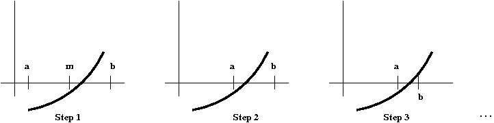
- At each step, reduce the size of the interval by half.
- Compute \(f(m)\) where \(m = \dv{(a+b)}{2}\).
- Decide whether to "move" \(a\) or \(b\) based on
whether \(m\) is on the same side of \(a\) or \(b\).
⇒
i.e., whether \(f(m)\) has the same sign as \(f(a)\) or \(f(b)\).
- Pseudocode:
     Algorithm: Bisection (a, b, f)
     Input: real numbers a,b where a < b, and function f
     1.    m = (a + b) / 2
     2.    while f(m) not close enough to zero
     3.        if f(m) < 0
     4.            a = m
     5.        else
     6.            b = m
     7.        endif
     8.        m = (a + b) / 2
     9.    endwhile
     10.   return m
- Sample Java code:
Bisection.java.
In-Class Exercise 4:
In the above example, we knew that \(f(a) \lt 0\). Re-write the
pseudocode to make it more general: replace the test
\(f(m)\lt 0\) with a test to see if \(f(a)\) and \(f(m)\)
are of the same sign.
Modify the code in
Bisection.java accordingly.
In-Class Exercise 5:
Examine the code in
Bisection.java:
- Use a calculator to compute \(\sqrt{3}\) and compare
with the output of the program. How would you increase the accuracy
of the program?
- Can the bisection() method be written recursively?
What would that do to efficiency?
1.2 Some interesting tidbits about real numbers
In no particular order, here are some interesting
facts about real numbers:
- What is an irrational number? A real number that's not rational.
- A rational can be expressed as a ratio of integers:
\(r = \dv{p}{q}\), where \(p, q\) are integers.
- How do we know irrational numbers exist? Example: \(\sqrt{2}\).
- Proof that \(\sqrt{2}\) is irrational:
- Assume that \(\sqrt{2}\) is rational.
- Express \(\sqrt{2}\) as \(r = \dv{p}{q}\) where the fraction
\(\dv{p}{q}\) cannot be reduced.
- Then, \(\dv{p^2}{q^2} = 2 \)
$$\eqb{
\implies & p^2 \eql 2 q^2 \\
\implies & p^2 \mbox{ is even}\\
\implies & p \mbox{ is even}\\
}$$
- By a similar argument (can you explain?), \(q\) is even.
⇒
Contradicts the assumption that the fraction is reduced.
- We know that rationals and integers are of the same cardinality.
⇒
The irrationals are uncountable.
- Most famous real number constants are irrational, e.g.
\(\pi, e\). (Proofs are not straightforward)
- Numbers that are solutions of some polynomial with integer coefficients are
called algebraic,
e.g., \(\sqrt{2}\) is the solution of \(x^2 - 2 = 0\).
- Another example: \(\Phi\), the golden ratio
is the solution to \(x^2 - x - 1 = 0\).
- Real numbers that are not algebraic are called
transcendental
e.g, \(\pi, e\)
- The real number system is unique:
- One can describe properties that define
the real number system.
⇒
For example: closure with respect to arithmetic, existence
of a least-upper-bound.
- One can show: any number system with these properties must
be equivalent to the real number system.
- The continuum hypothesis: there is no set whose countability
lies between that of the naturals and the reals.
What is known: cannot be proved or disproved using standard
set theory.
Ways of writing proofs:
- Even when the key idea in a proof makes sense, actually
writing the proof may not be trivial.
- For example: should there be a figure? should the proof
written free-flowing, like English text?
- Look at these variations of
proofs of the irrationality of \(\sqrt{2}\).
1.3 Sequences
Consider Zeno's paradox (circa 430 BC):
- To move from A to B, you must first reach the half-way point.
- But to reach the half-way point, you must first reach a
quarter of the distance.
- ... there are an infinite number of such moves.
⇒
Therefore, it's not possible to move to B.
Let's take a closer look:
In-Class Exercise 7:
Add the formula for \(S_{n}\) to
Zeno.java and compare
the for-loop sum (with 1 added) and the formula result.
Plot \(S_n\) vs. \(n\).
Now, let's examine a different sum:
- Define \(H_n \eql 1 + \frac{1}{2} + \frac{1}{3} + \ldots + \frac{1}{n}\)
- This is sometimes called the Harmonic sum, and
\(H_n\) is called the \(n\)-th Harmonic number.
In-Class Exercise 8:
Add code to
Harmonic.java and compare
the output from two computations: using double
vs. using float.
Try different value of \(n\). What do you think the
sum is converging to?
Plot \(H_n\) vs. \(n\).
In-Class Exercise 9:
Write code to compute \(A_n = (1 + \frac{1}{n})^n\) for
various values of \(n\).
Write your code in
the computeA() method of
SequenceExample.java.
Plot \(A_n\) vs. \(n\).
Let's make a few observations:
- These are the first few \(A_n\) values:
\(A_1 = 2, \; A_2 = 2.25, \; A_3 = 2.370370370, \;
A_4=2.44140625\)
- There are infinitely many \(A_n\)'s
because there are infinitely many values of \(n\).
⇒
\(A_1, A_2, A_3, \ldots\)
is called a sequence of numbers.
- Where there's no confusion, we'll use the terminology
"the sequence \(A_n\)" to mean the collection
of numbers (in order) \(A_1, A_2, A_3, \ldots\)
- Notice that \(H_n\) and \(S_n\) in the earlier
examples are also sequences.
What comes at the "end" of a sequence?
- Consider the simple sequence \(B_n = \frac{1}{n}\).
- For large \(n\), \(B_n\) is approximately 0.
- Now, there is no value of \(n\)
for which \(B_n = 0 \).
⇒
\(B_n\) gets closer and closer to 0 but never
actually "hits" 0.
- Similarly, the sequence
\(S_n = \frac{1}{2} + \frac{1}{4} + \ldots + \frac{1}{2^n}\)
gets closer and closer to 1.0 but never actually "hits" 1.0.
- In both cases, we say that the sequence has a limit.
- The limit of the sequence \(B_n\) is \(0\).
- The limit of the sequence \(S_n\) is \(1\).
- We write this as:
$$\eqb{
\lim_{n\to\infty} B_n & \eql & 0\\
\lim_{n\to\infty} S_n & \eql & 1
}$$
In-Class Exercise 10:
Write code in
SequenceExample2.java
to print the first few terms of the
sequence \(C_n = \frac{\sin(n)}{n}\).
How is this sequence different from the ones we've seen so far?
Some strangeness with limits:
- Because sequences can behave strangely, we need a more careful
definition of a limit.
- Wrong definition #1:
Each successive term is closer to the limit.
- Wrong definition #2:
Sequence \(X_n\) has limit \(L\) if the
distance \(X_n - L\) keeps decreasing.
- Wrong definition #3:
Given some arbitrarily small number \(\epsilon\), the
distance \(|X_n - L|\) is less than \(\epsilon\).
- Correct definition #1:
Given some arbitrarily small number \(\epsilon\), the
distance \(|X_n - L|\) is greater than \(\epsilon\)
only finitely many times.
- Correct definition #2:
For every small number \(\epsilon\),
\(|X_n - L| \; \lt \; \epsilon\)
for all large enough \(n\).
- Correct definition #3 (most common):
For every small number \(\epsilon\), there exists an integer \(N\)
such that
\(|X_n - L| \; \lt \; \epsilon\)
for all \(n \gt N\).
Informal version of last definition:
- For any "close-to-the-limit" distance \(\epsilon\),
you can go far enough down the sequence (large enough \(N\)
so that the rest of the sequence from there is
no further than \(\epsilon\) from the limit \(L\).
1.4 Random sequences
Consider the following code: (source file)
public class RandomSequence {

    public static void main (String[] argv)
    {
        for (int n=1; n<=10; n++) {
            System.out.println ("Un, n=" + n + ": " + computeU(n));
        }
    }

    static double computeU (int n)
    {
        return RandTool.uniform ();
    }

}
Note:
- This prints out a sequence of numbers, each of which is randomly
drawn from the range [0, 1].
- Let \(U_n\) denote this sequence.
- Let \(V_n \defn \frac{1}{n} (U_1 + U_2 + \ldots + U_n)\).
In-Class Exercise 11:
Write code
in RandomSequence2.java
to print the first 10 terms of the
sequence \(V_n\) defined above.
You will also need RandTool.java.
- Does the sequence \(U_n\) have a limit?
- Does the sequence \(V_n\) have a limit?
How are these sequences different from the ones we've seen before?
After writing your code to compute \(V_n\) above,
examine the code in
RandomSequence3.java.
What is the difference in the two approaches?
Next, we'll compute a few histograms:
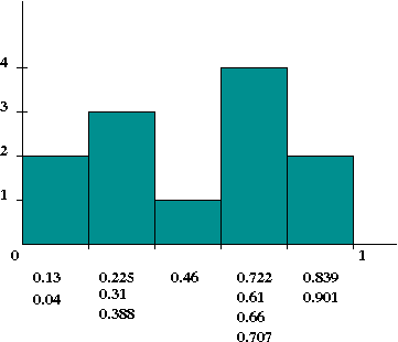
- What is a histogram?
Suppose we construct a 5-bin histogram on the interval [0,1].
- Consider this data set:
0.901, 0.13, 0.225, 0.46, 0.722, 0.61, 0.04, 0.3, 0.388,
0.839, 0.66, 0.707
- First, divide the range [0,1] into 5 intervals:
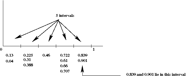
- Then, count the number of data items in each interval:
- We will write some code to compute a histogram for
values in the sequence \(U_n\).
(source file)
        // Create space: one counter per interval.
        int[] bins = new int [size];

        // Interval size.
        double interval = 1.0 / size;

        // Generate the data set, and identify the intervals.
        for (int k=0; k<numSamples; k++) {
            double u = computeU (n);                   // Get the n-th in sequence.
            int b = (int) Math.floor (u / interval);   // Which bin or interval?
            bins[b] ++;                                // Increment count accordingly.
        }
In-Class Exercise 12:
First, examine the
code in RandomSequence4.java
and verify that it prints out
possible random values, or samples, of \(U_5\).
Modify the code to print values of \(U_{493}\).
Next, download Histogram.java
and print a histogram for U5 with
different numbers of samples: 10, 100 and 10000.
What do you notice? Is it intuitive?
How do the histograms for \(U_5\)
differ from the equivalent histograms for \(U_{493}\)?
We need to point out a sublety:
- Consider the sequence \(U_n\)
- Each \(U_n\) is drawn randomly in the
interval \([0,1]\).
- Thus, for example, \(U_7\) does not
depend on the value of \(U_3\).
- However, is this property is true for the sequence \(V_n\)?
In-Class Exercise 13:
Modify Histogram.java
and to compute and print a histogram for \(V_n\) with
different numbers of samples: 10, 100 and 10000.
- How does the histogram for \(V_5\)
differ from the histogram for \(V_{493}\)?
- Print the histogram for \(V_{10000}\)
and explain the result.
A scaled sequence:
- Define the sequence \(W_n = \sqrt{n} (V_n - 0.5)\).
In-Class Exercise 14:
- First, let's get a feel for this by printing
out example values: add code in
RandomSequence5.java.
Does this appear to converge to a number for large values of \(n\)?
- Next, let's examine the histograms for various values of
\(n\).
Modify Histogram.java
and to compute and print a histogram for \(W_n\) with
different numbers of samples: 10, 100 and 10000.
- How does the histogram for \(W_5\)
differ from the histogram for \(W_{493}\)?
- Print and then plot the histogram for \(W_{10000}\).
- We'll now change the type of random generation.
In Histogram2.java,
create
a means of generating \(U_n^\prime\), a random
variable that's different from \(U_n\).
- Then, define \(V_n^\prime = \frac{1}{n}(U_1^\prime + \ldots U_n^\prime)\).
- Then, run your program to estimate what \(V_n^\prime\)
is converging to. Let's call this number \(\mu\).
- Now define \(W_n^\prime = \sqrt{n} (V_n^\prime - \mu)\).
- Plot the histograms for \(W_5^\prime\)
and \(W_{493}^\prime\).
The histograms of \(W_n\) and \(W_n^\prime\)
highlight one of the most important results in the history of science.
1.5 Two key ideas in the continous world: limits and continuity
Two important concepts pervade continuous mathematics:
- The idea of a limit (which we have just encountered).
- The idea of continuity
⇒ We will need to understand functions first.
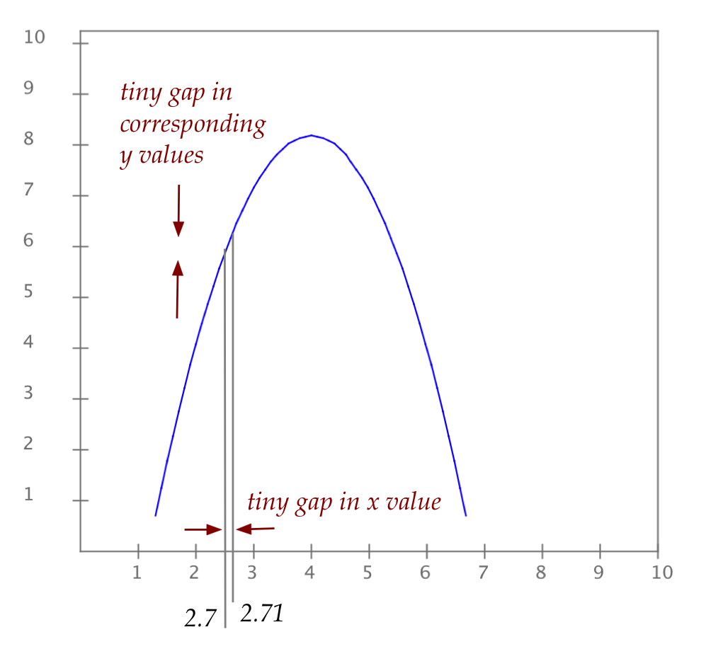
- The general idea in continuity: consider \(f(x) = 8 - (x-4)^2\)
- If you pick any
two values of \(x\) very close to each other,
e.g., \(x=2.7\) and \(x=2.71\)
⇒ Then, \(f(2.7)\) and \(f(2.71)\) are "close" for continuous functions.
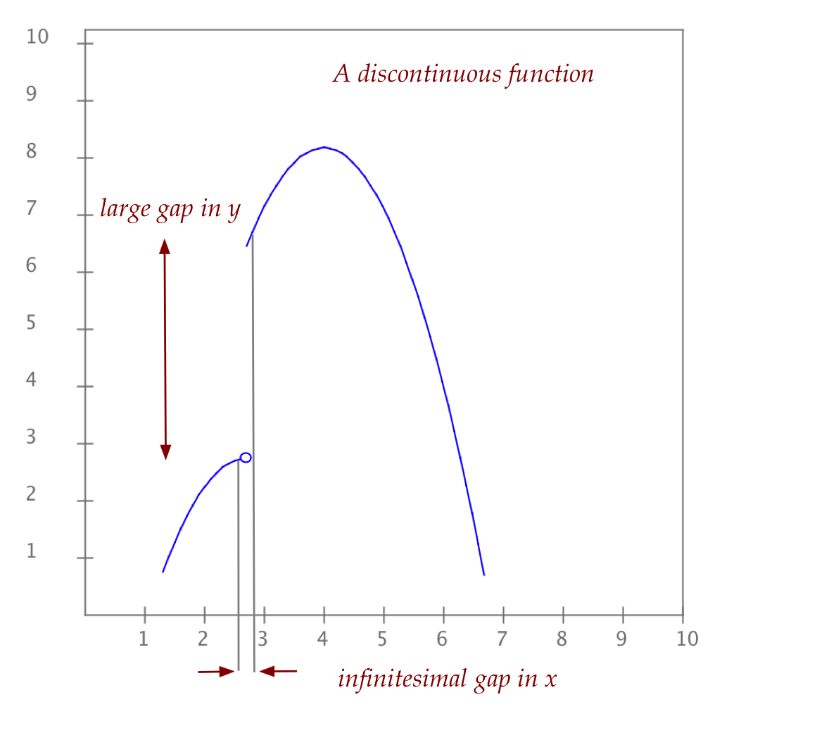
- In contrast, a discontinuous function will have
discontinuities somewhere, as in
About limits:
- Many key results in continuous mathematics are really limit results.
- Generally, limits simplify expressions, and
consequently, the mathematics.
- Generally, limits result in more powerful analytic tools.
- Although we never really reach "infinity", limits are
good approximations for large enough \(n\)
⇒
Sometimes, they're all we have.
- Theorems about limits aren't always easy to prove
⇒
But that shouldn't make the theorem statement hard to understand
- Always test a result with practical data or values before
using it.
About continuity:
- Continuity is usually a theoretical requirement to make
proofs work.
- Many real-world functions are actually "well-behaved"
(continuous) and, therefore, easy to work with.
- However, many are not - in these cases, we have to
struggle with each individual case.
⇒
It's almost always messy.
- Continuity can be explained in terms of limits:
- Suppose \(x_n\) is a sequence with limit
\(L\), and \(f(x)\) is a function.
- Then, consider the sequence of function values
\(f_n = f(x_n)\).
⇒
\(f_n\) is a sequence of real numbers.
- For a continuous function, the limit of \(f_n\)
is \(f(L)\).
1.6 Functions
What is a function?
- Engineers often think of a function as something that
takes an input value and produces an output:
- Mathematicians define it this way:
(e.g., Thomas and Finney. Calculus and Analytic Geometry )
A function from a set \(D\) to a set \(R\) is a rule
that assigns an element of \(R\) to each element in \(D\).
- The set \(D\) is often called the domain of the
function, meaning, the set of allowable input values.
⇒
We don't want inputs that are "bad"
- The set \(R\) is often called the range, the set
of possible outputs.
- For mathematical purity, we'd have to worry about whether
infinity is an allowed value or in the range
⇒
For most applications, we won't have to worry about such odd cases.
Exercise 15:
What types of "odd" cases do we have to worry about in real life?
Can you think of a function such that the number \(2\) is
a "bad" input value (i.e., shouldn't be allowed)?
Exercise 16:
Get out a piece of paper and draw (by hand) the function
\(f(x) = 3x^2+5\). What are the domain and range of this
function? How much of the domain and range did you sketch out?
Now let's write a simple program to compute
\(f(x) = 3x^2+5\):
(source file)
import java.util.*;

public class FunctionExample1 {

    public static void main (String[] argv)
    {
        // This is what reads from the keyboard:
        Scanner scanner = new Scanner (System.in);

        // Put out a prompt:
        System.out.print ("Enter x: ");

        // Read in a "double" (real) value:
        double x = scanner.nextDouble ();

        // Compute function:
        double f = 3*x*x + 5;

        // Print result (output):
        System.out.println (f);
    }

}
Exercise 17:
Download, compile and execute the above program,
FunctionExample1.java
to confirm your results from the previous exercise.
Exercise 18:
Modify the above program to compute the function
\(f(x) = \frac{1}{(x-2)}\). Use the program to generate
some values and draw a graph of the function.
What happens when \(x=2\)?
Next, let's write out several values using a loop:
(source file)
import java.util.*;

public class FunctionExample2 {

    public static void main (String[] argv)
    {
        System.out.println (" x   f(x)");         // Table header
        System.out.println ("---------");
        for (double x=1; x<=10; x=x+1) {
            double f = 3*x*x + 5;                 // Compute function.
            System.out.println (x + "  " + f);    // Print result.
        }
    }

}
Exercise 19:
Modify the above program to print out function values
for \(x\) in the range \([-10,-1]\).
We'll next graphically depict a function using a few points:
(source file)
import java.util.*;

public class FunctionExample3 {

    public static void main (String[] argv)
    {
        // Make a Function object and give it a name.
        Function F = new Function ("Silly function");

        for (double x=1; x<=10; x=x+1) {
            double f = 3*x*x + 5;
            // Feed the x,f(x) combinations into the object.
            F.add (x, f);
        }

        // Write to screen.
        System.out.println (F);

        // Display.
        F.show ();
    }

}
Exercise 20:
Modify the above program to show the shape of
the function \(f(x) = \frac{1}{(x-2)}\) in the range
\([0, 5]\). You will need to download
Function.java
and SimplePlotPanel.java.
Exercise 21:
For each of the functions below, generate 100 values
in the range \([0,10]\) and feed them into a
Function
object. Then, display the result.
- \(f(x) = 3x+5\)
- \(f(x) = x^2-2\)
- \(f(x) = \frac{5}{x^2}\)
- \(f(x) = e^{-2x}\)
Use
Function.show(F,G,...)
to plot multiple
Function's
together.
1.7 Distance between functions
"Comparison" vs. "distance":
- To see if \(f(x)\) "bigger" than \(g(x)\),
we can draw both and ask: in which intervals is \(f(x)\) bigger?
- This lets us compare functions just as we can compare numbers.
- Is there a function analog to the distance between two numbers?
- If there were, we could say function \(f(x)\) is "closer"
to function \(h(x)\) than \(g(x)\) is.
⇒
For example, is \(f(x)=3x+5\) closer to
\(h(x)=\frac{4}{x^2}\) or is \(g(x)=4e^{-2x}\) closer?
First, let's start examining "distance" by displaying two functions together:
- Let's draw \(f(x)=3x+5\) and \(g(x)=4x+5\).
- To do this, we'll generate 100 points in \([0,10]\)
for each function and display the results.
Here's the program:
(source file)
public class FunctionComparison {

    public static void main (String[] argv)
    {
        // Make two objects, one for each function.
        Function F = new Function ("3x+5");
        Function G = new Function ("4x+5");

        // Generate 100 values in the range [0,10]
        for (double x=0; x<=10; x+=0.1) {
            F.add (x, 3*x+5);
            G.add (x, 4*x+5);
        }

        // Display both together.
        Function.show (F, G);
    }

}
Exercise 22 :
Modify the above code to draw \(f(x)=3x+5\) and
\(g(x)=3x+10\) in the range \([0,10]\). Use only 50 points.
Next, we'll consider quantifying distance:
- We can quantify the distance between two numbers:
⇒
The distance between numbers \(12.33\) and \(10.01\) is
\(12.33 - 10.01 = 2.32\).
- Can we apply the "subtraction" idea to functions?
- One way to do this:
Let's write a small program to compute the "distance" between
\(f(x)=3x+5\) and \(g(x)=3x+10\).
- We'll identify 50 x-values on the x-axis and take the
difference between the two functions at these x-values.
- We'll sum up these differences.
Here's the program:
(source file)
public class FunctionComparison2 {

    public static void main (String[] argv)
    {
        // Initialize sum.
        double distance = 0;

        // Generate 50 values in the range [0,10]
        for (double x=0; x<=10; x+=0.2) {
            double f = 3*x + 5;
            double g = 3*x + 10;
            double diff = g - f;
            distance = distance + diff;
        }

        System.out.println ("Distance: " + distance);
    }

}
Exercise 23:
Did it matter whether we used \(g-f\) or \(f-g\) above?
What is the distance between the functions \(f(x)=3x+5\)
and \(h(x)=20\)? What happens when you use \(f-h\)
vs. \(h-f\)?
Exercise 24:
Coding exercise: modify the above example so that the loop
has only one line of code (and is therefore more compact).
Exercise 25:
Modify the example to use 100 points (in
the same range [0,10]) instead of 50.
What do you notice? What does this tell you about the
method we're using to compute distance?
Consider the following modification:
(source file)
public class FunctionComparison3 {

    public static void main (String[] argv)
    {
        // Initialize sum.
        double sum= 0;

        // Generate 50 values in the range [0,10]
        for (double x=0; x<=10; x+=0.2) {
            double f = 3*x + 5;
            double g = 3*x + 10;
            sum += Math.abs (f - g);
        }

        // Compute the average distance:
        double distance = sum / 50;

        System.out.println ("Distance f to g: " + distance);
    }

}
Note:
- We have now used an average of the distances instead of the sum.
Exercise 26:
Modify the above example as follows:
- First, use 100 points instead of 50. Then use 1000 points.
What do you observe?
- Next, change the range from \([0,10]\) to \([0,5]\).
What is the distance between \(f\) and \(g\) using this range?
- Repeat the above for \(f\) and \(h(x)=20\). Does the
distance measure for functions make sense?
Finally, consider this variation of measuring functional distance:
(source file)
public class FunctionComparison4 {

    public static void main (String[] argv)
    {
        // Initialize sum.
        double sum= 0;

        // Generate 50 values in the range [0,10]
        for (double x=0; x<=10; x+=0.2) {
            double f = 3*x + 5;
            double g = 3*x + 10;
            sum += Math.abs (f - g);
        }

        // Compute the average distance, multiplied by length of interval:
        double distance = (10-0) * sum / 50;

        System.out.println ("Distance f to g: " + distance);
    }

}
Note:
- Here, we have multiplied the distance by the size of the range.
Exercise 27:
Now modify the above example to use \([0,5]\) as the range:
- What is the distance between \(f\) and \(g\) using this range?
- Next, use 100 points instead of 50. Then use 1000 points.
Is our modified measure severely affected by the number of points?
Let's re-write the above code slightly:
(source file)
public class FunctionComparison5 {

    public static void main (String[] argv)
    {
        // Initialize sum.
        double sum= 0;

        // Compute interval = range/number-of-points:
        double interval = (10.0 - 0.0) / 50.0;

        // Generate 50 values in the range [0,10]
        for (double x=0; x<=10; x+=0.2) {
            double f = 3*x + 5;
            double g = 3*x + 10;
            sum += interval * Math.abs (f - g);
        }

        System.out.println ("Distance f to g: " + sum);
    }

}
Exercise 28:
Why does this produce exactly the same result?
Exercise 29:
Coding exercise: Change the second line to
double interval = (10 - 0) / 50;
Then compile and execute - what do you observe? Explain.
We can use our distance measure to compute the distance
of a function from the x-axis:
⇒
The x-axis is merely the function \(z(x) = 0\).
Here's an example:
(source file)
public class FunctionComparison6 {

    public static void main (String[] argv)
    {
        // Initialize sum.
        double sum= 0;

        // Compute interval = range/number-of-points:
        double interval = (10.0 - 0.0) / 50.0;

        // Generate 50 values in the range [0,10]
        for (double x=0; x<=10; x+=interval) {
            double f = 3*x + 5;
            double z = 0;
            sum += interval * Math.abs (f - z);
        }

        System.out.println ("Distance f to x-axis: " + sum);
    }

}
Exercise 30:
Consider the function \(h(x)=20\) in the range
\([0,10]\). Draw this on paper - you should have a rectangle
of width \(10\) and height \(20\).
Next, use 4 equally-spaced
x-values and hand-execute the above program with \(h(x)\) instead
of \(f(x)\). Can you relate
the calculations to the area of the rectangle?
Exercise 31:
Now consider the function \(f(x)=3x+5\) in the range
\([0,10]\). Draw this on paper and repeat the
above steps (using 4 intervals) to compute the distance
to the x-axis. How does this relate
to the area? What happens when we use more intervals
(e.g., 50 intervals)? Try 50 intervals, then try 1000 intervals.
Can you calculate the area exactly by hand?
Exercise 32:
Draw the two functions \(f(x)=3x+5\) and \(g(x)=20\)
on paper. What is the relationship between our distance
measure and area?
1.8 Sine's and signs
Let us revisit some elementary trigonometry:
Let's write a program to print out some values of these functions:
(source file)
public class SinCos {

    public static void main (String[] argv)
    {
        // First, some sin examples;
        double s = Math.sin (0);
        System.out.println ("sin(0)=" + s);
        s = Math.sin (Math.PI/2);
        System.out.println ("sin(pi/2)=" + s);
        s = Math.sin (Math.PI/4);
        System.out.println ("sin(pi/4)=" + s);

        // Now some cos examples:
        double c = Math.cos (0);
        System.out.println ("cos(0)=" + c);
        c = Math.cos (Math.PI/2);
        System.out.println ("cos(pi/2)=" + c);
        c = Math.cos (Math.PI/4);
        System.out.println ("cos(pi/4)=" + c);
    }

}
Exercise 34:
Modify the above program to print out \(\sin(\frac{4\pi}{3})\)
and answer the following:
- Why is the result negative? What does it have to do with
actual angles and our earlier definition of the \(\sin\)
function?
- Convert the angle from radians to degrees (perhaps by
modifying the program). Draw the result on paper.
See if this helps answering the above question.
- Modify the code to print out \(\sin(2\pi + \frac{4\pi}{3})\).
Can you explain the result?
We'll now write code to draw the functions in the
range \([0, 8\pi]\):
(source file)
public class SinCos2 {

    public static void main (String[] argv)
    {
        // Create two Function objects.
        Function sinFunc = new Function ("sin");
        Function cosFunc = new Function ("cos");

        // Put values into them.
        for (double x=0; x<=8*Math.PI; x+=0.1) {
            sinFunc.add (x, Math.sin(x));
            cosFunc.add (x, Math.cos(x));
        }

        // Display.
        Function.show (sinFunc, cosFunc);
    }

}
Exercise 35:
Explain why both functions are periodic (that is,
the structure repeats). What is the period (the
size of the interval after it repeats)?
We will now try to find the maximum value of the \(\sin\)
function in the range \([0,2\pi]\):
- The graph shows that the maximum is 1.
- If we didn't know, we could write a small program to
find the maximum:
(source file)
public class SinMaximum {

    public static void main (String[] argv)
    {
        // Initial guess: max occurs at 0, and has value 0.
        double bestX = 0;
        double max = Math.sin (bestX);

        // Now try values in the range [0,2*pi]
        for (double x=0; x<=2*Math.PI; x+=0.1) {
            double f = Math.sin (x);
            if (f > max) {
                max = f;
                bestX = x;
            }
        }

        // Print result.
        System.out.println ("Max value " + max + " occurred at x=" + bestX);
    }

}
Exercise 36:
Use the above approach to find the minimum value of \(\cos(x)\) for \(x\)
in the range \([0, 2\pi]\). What could we do to make the result
more accurate?
1.9 Guessing Functions
Often we have data and want a rule that explains the data:
- We want to decipher or extract the function that
relates the data.
- Example: suppose we have this data:
| x | f(x) |
| 1 | 1 |
| 2 | 4 |
| 3 | 9 |
| 4 | 16 |
| 5 | 25 |
⇒
Then we could easily determine \(f(x) = x^2\).
- Is it so obvious if the data were:
| x | f(x) |
| 1.5 | 2.25 |
| 2.33 | 5.4289 |
| 2.71 | 7.3441 |
| 4.6 | 21.16 |
| 5.3 | 28.09 |
Exercise 37:
What good are such "rules"? Why are they useful?
Why not just use the data directly?
Exercise 38:
Can you guess the function that produced this data:
| x | f(x) |
| 1.0 | 5.86 |
| 2.0 | 9.00 |
| 3.0 | 12.14 |
| 4.0 | 15.28 |
| 5.0 | 18.43 |
| 6.0 | 21.57 |
Techniques for guessing functions:
- A first step is to see if the data can be reasonably
approximated by a linear function such as \(f(x)=3x+5\).
- If so, we try to find values \(a\) and \(b\)
so that \(f(x)=ax+b\) best explains the data.
- For example, consider the data
| x | f(x) |
| 1.0 | 8.0 |
| 2.0 | 11.00 |
| 3.0 | 14.00 |
| 4.0 | 17.00 |
| 5.0 | 20.00 |
- We will first display the data to get a "feel" for the shape
of the function:
(source file)
public class DataAnalysis {

    public static void main (String[] argv)
    {
        // Make a Function object.
        Function F = new Function ("mystery");

        // Put the data in.
        F.add (1, 8);
        F.add (2, 11);
        F.add (3, 14);
        F.add (4, 17);
        F.add (5, 20);

        // Display it.
        F.show ();
    }

}
- Now that we know that it's linear, i.e., of
the form \(f(x)=ax+b\) how do we discover \(a\) and \(b\)?
This is where a little math will be useful.
- Consider two points \(x_1\) and
\(x_2\) in the data.
- For example, \(x_1 = 1\) and
\(x_2 = 2\) (the first two x-values).
- For \(x_1 = 1\), we know that
\(f(x_1) = ax_1+b\) must equal \(8\).
⇒
\(ax_1+b = 8\)
⇒
\(a + b = 8\)
- Similarly, for the second point
⇒
\(ax_2 + b = 11\)
⇒
\(2a + b = 11\)
- Subtracting the first equation from second gives us \(a =
3\), which means \(b = 5\).
Exercise 39:
Identify the linear function in the previous exercise.
Exercise 40:
Draw the graph for this data:
| d | v |
| 8.33 | 1666.67 |
| 22.22 | 3666.67 |
| 23.61 | 4833.33 |
| 30.55 | 5000 |
| 36.81 | 5166.67 |
| 47.22 | 8000 |
| 69.44 | 11333.33 |
| 105.56 | 19666.67 |
Is the curve linear or non-linear? The data is from a historic 1929 paper.
What if the data is obviously "noisy" (has errors)?
- There are well-established techniques for fitting
linear functions to noisy data.
⇒
Example: least-squares regression
- Key idea: find the line so that the "distance"
from data points to the line is minimized.
⇒
The "distance" measure is very similar to the one we used earlier.
Exercise 41:
Draw the graph for this data:
| x | f(x) |
| 1.0 | 1 |
| 2.0 | 13 |
| 3.0 | 33 |
| 4.0 | 61 |
| 5.0 | 97 |
Is the curve linear or non-linear?
What if the data is obviously non-linear?
- Non-linear functions are hard to fit to data.
- If the underlying function has a simple form, such as
\(f(x) = ax^2\), it is easy.
- However, non-linear functions can be quite complicated.
⇒
This is a sub-area called interpolation or curve-fitting.
1.10 Dealing with Nonlinearity
One way to get a grip around nonlinearity is to transform
the data or your guessed function:
- For example, consider the following data:
| x | f(x) |
| 0.5 | 4.97 |
| 1.5 | 4.77 |
| 2.5 | 4.33 |
| 3.5 | 3.57 |
| 4.5 | 2.18 |
- This is an example of transforming the data
to see a pattern (and infer an underlying function).
One way of transforming a function is to study its derivative:
- Consider some function \(f(x)\) and some particular value
of \(x\) such as \(x=5\).
- Suppose we pick some small value such as \(0.01\) and
compute the following:
- Compute \(f(5 + 0.01)\)
- Compute \(f(5)\)
- Then compute \( \frac{f(5.01) \; - \; f(5)}{(5.01 \; - \; 5)}\).
This value answers the question: if you move along the x-axis
from \(5\) to \(5.01\) (a small step), how much
does \(f\) change?
- Notice: this defines "change" starting at \(5\).
⇒
At the x-value of \(6\), the change would be
\(\frac{f(6.01) \; - \; f(6)}{6.01 \; - \; 6}\).
- In more general terms, the change at some value \(x\) is:
\(\frac{f(x+0.01)\; - \; f(x)}{0.01}\).
- What is so special about \(0.01\)?
Nothing. We should really define "change" at \(x\) as:
\(\frac{f(x+d) \; - \; f(x)}{d}\).
- We could use \(d=0.01\) or \(d=0.0000001\) or
whatever's appropriate, depending on our needs.
- Notice that the result is a number.
- There is one such number for every \(x\) and \(d\).
- Thus, the output is a function of \(x\) and \(d\):
- For a fixed value of \(d=0.01\) (for example), each input
\(x\) results in a output number \(\frac{f(x+0.01) \; - \; f(x)}{0.01}\).
- Thus, the computation is a function.
- Let's give this function a name: \(g(x) = \frac{f(x+0.01) \;
- \; f(x)}{0.01}\).
- Let's look an example:
- Consider the function \(f(x) = 3x^2\).
- We'll write a program to compute \(g(x) = \frac{f(x+0.01) \;
- \; f(x)}{0.01}\):
(source file)
public class Diff {

    public static void main (String[] argv)
    {
        // The value of d is fixed throughout.
        double d = 0.01;

        // Compute for x-values in [0,10]
        for (double x=0; x<=10; x+=1) {
            // Compute f.
            double f = 3*x*x;

            // Compute (f(x+d) - f(x)) / d
            double f_xd = 3 * (x+d)*(x+d);
            double g = (f_xd - f) / d;

            // Print.
            System.out.println ("x=" + x + "  g(x)=" + g);
        }
    }

}
- This type of transformation of a function is called
a derivative

- There is a more precise mathematical definition, which we
will defer to later.
Exercise 43:
Execute the above program, Diff.java.
Does the function \(g(x)\)
look familiar? Modify the above code to fill in the \(f\) and \(g\) values
into Function objects and display them.
Exercise 44:
- Use \(d=0.01\) and plot the derivative function \(g(x)\)
along with \(f(x)\) when \(f(x)=3x^2 + 5\).
- Compare this derivative function with that of \(f(x)=3x^2\).
Explain what you observe.
- Use two points on the derivative function and write down
the function as a formula.
- Explore what happens with different \(d\) values, for
example try \(d=1, d=0.1, d=0.0001, d=0.00001\).
Reconstructing the original function:
- Suppose I know the derivative function \(g(x)\), can
I reconstruct the original \(f(x)\) such that
\(g(x) = \frac{f(x+d) \; - \; f(x)}{d}\)?
- We can re-arrange the above to see that
\(f(x+d) = f(x) + d g(x)\)
- But how do we know the \(f(x)\) on the right side?
- As a first step, suppose we happen to know \(f(0)\).
- Then we can compute \(f(0+d) = f(0) + d g(0)\).
⇒ We know \(g(x)\), remember?
- Now that we know \(f(d)\), we can compute
\(f(d+d) = f(d) + d g(d)\).
- Now that we know \(f(2d)\), we can compute
\(f(3d) = f(2d) + d g(2d)\).
- ... and so on until we have a whole bunch of values of \(f\).
- Let's see how this works in an example:
- Suppose we know the derivative function is \(g(x)=6x\)
and that \(f(0)=0\).
- We want to ask: what function \(f(x)\) is such that
its derivative is \(g(x)=6x\)?
- Let's write a program to successively compute \(f(d),
f(2d), f(3d), f(4d), ....\):
(source file)
public class Integration {

    public static void main (String[] argv)
    {
        // The value of d is fixed throughout.
        double d = 0.01;

        // Initial value is assumed known:
        double f = 0;

        // Compute for x-values in [0,10]
        for (double x=0.01; x<=2; x+=0.01) {
            // We are given g, so we can compute it.
            double g = 6 * x;

            // Find the new value at f(x+d) that becomes the new f.
            f = f + d * g;

            // Print.
            System.out.println ("x=" + x + "   f(x)=" + f);
        }
    }

}
- Suppose we wanted to compute \(f(x)\) at some
particular value of \(x\), for example, \(x=3\).
- We would still need to start at \(d=0\), and
compute \(f(d), f(2d), f(3d), ....,\), until we
"hit" \(f(3)\).
- Let's re-arrange the code to compute \(f(x)\) at
any desired value:
(source file)
public class Integration2 {

    public static void main (String[] argv)
    {
        // We'll compute f(x) at x=1, 2, ..., 10 and put that in a graph.
        Function F = new Function ("f");

        // Notice: we are computing f(1), f(2), ..., and NOT f(d), f(2d), ...
        for (double x=1; x<=10; x+=1) {
            // Our method compute_f() does all the dirty work.
            double f = compute_f (x);
            F.add (x, f);
            System.out.println ("x=" + x + "  f(x)=" + f);
        }

        // Display.
        F.show ();
    }


    static double compute_f (double x)
    {
        // The value of d is fixed throughout.
        double d = 0.01;

        // Initial value is assumed known:
        double f = 0;

        // Compute for x-values in [0,10]. We are now using a variable called z.
        // Notice: goes over the range 0.01 up through x (which is input to the method).
        for (double z=0.01; z<=x; z+=0.01) {
            // We are given g, so we can compute it.
            double g = 6 * z;

            // Find the new value at f(z+d) that becomes the new f.
            f = f + d * g;

            // No need to print intermediate values.
        }

        // Return f(x)
        return f;
    }

}
Exercise 45:
Suppose the derivative of \(f(x)\) is \(g(x)=-sin(x)\)
and that we know \(f(0)=1\).
Modify the above code to compute \(f(x)\) in the interval
\([0,2\pi]\) and display the result.
Working with a simulation:
- Suppose we were able to simulate some physical system of interest.
- Let's say that we are interested in the relationship
between two variables \(x\) and \(y\).
⇒
We want to figure out the function \(f\) such that \(y = f(x)\).
- If the relationship is nonlinear, we can try to use
derivatives to see if that helps.
- For example, suppose our simulation was a piece of
software called Simulator:
(source file)
public class UnknownFunctionDerivative {

    public static void main (String[] argv)
    {
        // Make an instance of the object.
        Simulator S = new Simulator ();

        double d = 0.01;

        for (double x=0; x<=10; x+=1) {
            // Compute derivative at x.
            double f = S.getValue (x);
            double fd = S.getValue (x+d);
            double g = (fd - f) / d;
            System.out.println ("x=" + x + "  g(x)=" + g);
        }

    }

}
Exercise 46:
Download Simulator.class
and UnknownFunctionDerivative.java,
and execute. What is the relationship between \(x\) and \(f(x)\)?
1.11 Computing and storing functions
First, consider how functions are specified:
- If the domain is discrete and finite, we could simply list
function values:
- For example
| d | v |
| 8.33 | 1666.67 |
| 22.22 | 3666.67 |
| 23.61 | 4833.33 |
| 30.55 | 5000 |
| 36.81 | 5166.67 |
| 47.22 | 8000 |
| 69.44 | 11333.33 |
| 105.56 | 19666.67 |
- Here, \(v\) is a function of \(d\), but there are
only finitely many values
⇒
One can list all of them.
- For an uncountable domain, this is impossible
⇒
Must have use some other means
⇒
function is specified by construction, e.g.,
\(f(x) = 3x^2 + 5\).
There are several different ways of writing code to compute functions:
- If the functional form is known, simply implement the code
to compute, e.g., for \(f(x)=3x^2+5\)
    double computef (double x)
    {
        return 3*x*x + 5;
    }
- If an approximate functional form is known, write code
to implement the approximation:
- If no functional form is known, we might have some sample
points:
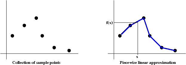
In this case, the approximate function might suffice.
- Sometimes we have sample points, but can construct a
smoother curve
⇒
Use curved interpolating segments (e.g., Bezier curves)
Exercise 48:
Download AccelCar.java,
Function.java
and SimplePlotPanel.java.
This is a simple model of an accelerating vehicle - the goal
is to start at the left and reach the right in the least
time possible but also such that the velocity at the
end is as close to zero as possible.
- Compile and
execute AccelCar,
and try to achieve as low a score as possible.
- Then try to determine a good acceleration "function" by hand
by reasoning.
- Download MyController.java,
compile and execute. Examine the code - you should see a sample
acceleration function.
- Implement a better acceleration function in
MyController.
- How would you systematically search for the optimal acceleration function?
1.12 Limits of functions
A sequence of functions:
- We've seen examples of sequences of real numbers
⇒
e.g., \(C_n = \frac{\sin(n)}{n}\).
- Consider the function \(f_n(x) = \frac{x^2}{n}\)
in the interval \([0,1]\).
- The functions
\(f_1(x) = x^2\)
\(f_2(x) = \frac{x^2}{2}\)
\(f_3(x) = \frac{x^2}{3}\)
. . .
form a sequence of functions.
- The limit of a sequence of functions is itself a function.
- Some of the most important results in mathematics arise
from limits of functions.
⇒
Often the limiting function is more useful and practical
- Example: the Central Limit Theorem.
- The derivative function is an example of a limiting
function:
- For a function \(f(x)\), define
\(g_d(x) = \frac{f(x+d) \; - \; f(x)}{d}\).
- Then, as \(d \to 0\), we get a sequence of functions.
- The derivative is defined as the limit of this sequence:
\(f'(x) = \lim_{d\to 0} g_d(x) =
\lim_{d\to 0} \frac{f(x+d) \; - \; f(x)}{d}\).
Exercise 49:
Construct a sequence of distinct functions so that the limit
is \(f(x)=x\).
© 2008, Rahul Simha