Our goals in this module are:
- To walk in Newton's footsteps, to see
how basic questions about motion drove the development of calculus.
- To see how a physical simulation can be used to explore and discover.
- To learn how to write such simulations.
Let's start with some (Galileo-like) exploration.
Exercise 1:
Download and execute Incline.java.
This is a simulation of a bead falling along an inclined
wire with no friction. You can set the incline angle and
also the mass of the bead. Use your own watch/timer and
your own observations with pen-and-paper of the executing simulation (that is,
don't write code) to answer these questions:
- Estimate the distance traveled in 1 second, in 2 seconds, 3
seconds ... etc. That is, sketch out a graph with time on the
x-axis and distance (along incline) along the y-axis.
- Estimate the velocity between successive tick marks along
the incline. That is, what is the velocity between the
first two tick marks, between the second two, ... etc.
- How do these graphs change if you double the mass?
- How do these graphs change if you double the angle?
From these observations (only) what can you conclude about
the relationship between:
- Distance traveled and time?
- Velocity and time?
- Mass and distance traveled?
- Angle and distance traveled?
Let us use a more refined tool that will allow more accurate
measurements:
- Suppose we have a measurement device capable of very
accurate measurements:
⇒
You set a "time" and it returns the distance traveled.
- We will use one such "virtual measurement device"
⇒
A simulator.
- Here is how we'd use a simulator for the incline problem:
(source file)
public class InclineSimulatorExample {

    public static void main (String[] argv)
    {
        // Make an instance of the simulator.
        InclineSimulator sim = new InclineSimulator ();

        // Set mass and angle.
        sim.mass = 1;
        sim.angle = 30;

        // We'll measure distance travelled at t=1, t=2, ... and put
        // these values into a Function object.
        Function dist = new Function ("dist");

        for (double t=1; t<=10; t+=1) {
            double d = sim.run (t);
            dist.add (t, d);
        }

        // Display result.
        dist.show ();
    }

}
Exercise 2:
Download InclineSimulatorExample.java,
InclineSimulator.java,
Function.java, and
SimplePlotPanel.java.
Then, compile and execute InclineSimulatorExample.
What do you observe is the relationship between distance and time?
Exercise 3:
Modify the code in InclineSimulatorExample.java
to compute the derivative at \(t=1, 2\) ... etc. For example, to
estimate the derivative at \(t=2\), you would
- Obtain \(d\), the distance traveled in 2 seconds.
- Obtain \(d'\), the distance traveled in 2.01 seconds.
- Estimate the derivative at \(t=2\) as \((d'-d)/0.01\).
What do you conclude from estimating the derivative?
Repeat the derivative estimation using \(0.0001\) instead of \(0.01\).
Can you explain what you observe?
Let's next explore the idea of instantaneous velocity:
- In the above exercise, we measured the distance-derivative as:
\((d'-d)/0.01\)
- If \(d(t)\) is the function that describes distance in
terms of time, then the derivative at time \(t\) is
estimated as $$\frac{d(t + 0.01) - d(t)}{0.01}$$.
- But \(d(t+0.01) - d(t)\) is the distance traveled in the
time interval \(0.01\)
⇒
It's short, to be sure, but a non-zero distance nonetheless.
⇒
The velocity in that interval is distance-traveled / time-taken
⇒
velocity = \(\frac{d(t + 0.01) - d(t)}{0.01}\).
- We will call this the instantaneous velocity at time \(t\).
- If we used \(0.001\) instead of \(0.01\), the result
would be "even more instantaneous".
- Another way to describe it is this mouthful: instantaneous rate-of-change of distance
Exercise 4:
Consider the function \(f(x) = 3x+5\). Use \(0.1\) and
compute the instantaneous rate-of-change at \(x=1\), at \(x=2\),
and \(x=3\). Then use \(0.01\) and compute the same.
What do you conclude? What can you conclude about the instaneous
rate-of-change of any linear function \(f(x) = ax+b\)?
About instantaneous rate-of-change:
- For linear functions, there's a nice pictorial
view of what this means:
- For a nonlinear function, it's a little more
complicated:
Let's take a closer look at instantaneous velocity
in our incline-simulator:
- The instantaneous velocity is itself a function of time:
⇒
For every time \(t\), we define the instantaneous-velocity
as $$\frac{d(t+0.01) - d(t)}{0.01}$$.
- Let's give this function a name:
$$v(t) \eql \frac{d(t+0.01) - d(t)}{0.01}$$.
- The simulator has been written to provide instantaneous
velocity whenever you want it:
(source file)
public class InclineVelocityExample {

    public static void main (String[] argv)
    {
        // Make a new instance of the class. Set mass and angle.
        InclineSimulator sim = new InclineSimulator ();
        sim.mass = 1;
        sim.angle = 30;

        Function velocity = new Function ("velocity");

        for (double t=1; t<=10; t+=1) {
            // Run simulator up to time t.
            sim.run (t);
            double v = sim.getV ();
            velocity.add (t, v);
        }

        // Display result.
        velocity.show ();
    }

}
- Suppose we try to compute the derivative of instantaneous velocity
$$\frac{v(t+0.01) - v(t)}{0.01}$$
Exercise 5:
Execute the above code and estimate the slope (by hand, looking at the graph).
Then modify the code to estimate the derivative of the velocity
function at \(t=1, t=2, ..., t=10\).
Acceleration:
- We will give a shorter name to instantaneous rate-of-change
of velocity
⇒
It's called acceleration
- Since there is a value of this acceleration at each moment,
it is really a function
⇒
\(a(t) = \) acceleration at time \(t\).
Exercise 6:
At this point we might try formulating a general "law"
about motion:
- How would you state the law?
- How is the acceleration (velocity-derivative or instantaneous rate-of-change
of velocity) affected by the mass of the bead? Try different
mass values (1, 2, 3, etc).
- How is acceleration affected by the angle?
Try angles of 10, 20, ..., 80. (You might have to re-size
the window).
- What can we say about a universal law at this time?
3.2 Formulating a Universal Law - More Examples
A simpler experiment:
- Consider dropping a ball from a height.
- Let \(d(t) = \) height of ball above ground after
\(t\) seconds.
- Once again, suppose we have a simulator that returns
the height after a given time, we could use it as follows:
(source file)
public class BallDropSimulatorExample {

    public static void main (String[] argv)
    {
        BallDropSimulator sim = new BallDropSimulator ();

        Function dist = new Function ("distance");

        for (double t=1; t<=10; t+=1) {
            // Drop from a height of 1000
            double d = sim.run (t, 1000);
            dist.add (t, d);
        }

        dist.show ();
    }

}
Exercise 7:
Execute the above code. You will also need
BallDropSimulator.java.
- Modify the the code in main to estimate the velocity curve.
- Write code to estimate the slope of the velocity curve.
- Thought exercise: picture yourself in the times of Newton (mid 1600's).
How would you perform an experiment to measure \(d(t)\) for
a falling object? What was the clock technology like at that time?
A variation:
- Toss a ball upward with some initial velocity.
- Let \(d(t) = \) height of ball after \(t\) seconds.
- If we have a simulator, we would use it as follows:
(source file)
public class BallTossSimulatorExample {

    public static void main (String[] argv)
    {
        BallTossSimulator sim = new BallTossSimulator ();

        Function dist = new Function ("distance");

        for (double t=1; t<=10; t+=1) {
            double d = sim.run (t, 50);
            dist.add (t, d);
        }

        dist.show ();
    }

}
Exercise 8:
Execute the above code. You will also need
BallTossSimulator.java.
Then, modify the the code in main to estimate
the velocity curve. What can you conclude about your
universal law thus far?
Next, let's consider projectile motion:
- Suppose we try to analyze the distance moved along the
projectile's curve:
⇒
Let \(d(t) =\) distance moved along curve.
- Let's ask whether our "universal law" holds
⇒
Is velocity linear? Is acceleration constant?
- For this purpose, we will use a simulation of
the projectile, written in ProjectileSimulator.java.
- Thus, to plot the distance travelled (the \(d(t)\)
function):
(source file)
public class ProjectileSimulatorExample {

    public static void main (String[] argv)
    {
        // Make a new simulator object.
        ProjectileSimulator proSim = new ProjectileSimulator ();

        // We want to plot d vs. t
        Function dist = new Function ("distance");

        for (double t=0.1; t<=2.3; t+=0.1) {
            // mass=1, angle=37, initVel=20
            // Simulator accuracy: 0.0001
            double d = proSim.run (1, 37, 20, t, 0.0001);
            dist.add (t, d);
        }

        // Display.
        dist.show ();
    }

}
Exercise 9:
Download ProjectileSimulator.java
and then modify
ProjectileSimulatorExample.java
to compute the distance and velocity functions,
\(d(t)\) and \(v(t)\). Use \(s=0.01\) and,
for the derivative of velocity, use \(v'(t)=(v(t+0.1) - v(t)) / 0.1\)
for acceleration.
Try this once with angle=37 and once with angle=70.
What do you conclude from observing \(d(t)\)?
What can you conclude about the rate of change of velocity?
3.3 Going the Other Way - from Acceleration to Distance
Before looking further into our universal law, let us take
a closer look at the relationship between acceleration, velocity,
and distance
⇒
Our law must somehow account for these quantities.
Reconstructing motion from acceleration:
- Suppose we know that acceleration is constant, could
we reconstruct motion (the distance function)?
- This is what we know:
- The derivative of the distance-function \(d(t)\) is:
the velocity function \(v(t)\).
- The derivative of the velocity-function \(v(t)\)
is: the acceleration function \(a(t)\).
- What we'd like to do: construct \(d(t)\) when
we know (or are given) \(a(t)\).
- For example, if \(a(t)=5\) (constant acceleration),
then what is \(d(t)\)?
- Let us follow the approach in Module 1:
- We know that $$a(t) \eql \frac{v(t+s) - v(t)}{s}$$ for some
small value \(s\) (e.g., \(s=0.01\)).
- Then, rearranging gives us $$v(t+s) \eql v(t) + s \; a(t)$$
- Suppose we know \(v(0) = 0\).
⇒
(Turns out, we have to know the initial value.)
- Then, we could compute $$v(0+s) \eql v(0) + s \; a(0)$$
- We can now compute \(v(t)\) at \(t=2s, 3s, 4s, \ldots\)
$$\eqb{
v(s + s) & \eql & v(s) + s \; a(s) \\
v(3s) & \eql & v(2s) + s \; a(2s) \\
v(4s) & \eql & v(3s) + s \; a(3s) \\
& \vdots &
}$$
- In code, we would want to write
next-\(v\)-value = previous-\(v\)-value + \(s \; \times \; \) previous-acceleration-value
- If we update \(t\) as we proceed, we could write
$$\eqb{
v^\prime & \leftarrow & v + s \; a(t) \\
t & \leftarrow & t + s
}$$
Exercise 10:
Suppose \(a(t)=4.9\) (acceleration is a constant value
of \(4.9\)), and that initial velocity is zero.
- Draw a graph of \(a(t)\) in the range \([0,10]\).
- Use \(s=0.1\) and compute by hand \(v(0.1), v(0.2), v(0.3),
v(0.4), v(0.5)\). Show your calculations.
- Explain why the value for \(v(0.5)\) makes sense.
- What is the connection between the calculations you did
and the terms "line" and "slope"? What is the equation of
the line in question?
Next, let's write a small program to compute \(v(t)\):
- We'll use \(a(t)=4.9\) as an example.
- Here's the program
(source file)
public class IntegrateAccel {

    public static void main (String[] argv)
    {
        // a(t) = 4.9 (constant acceleration).
        double a = 4.9;

        // Initial velocity.
        double v = 0;

        // Our small "change" interval
        double s = 0.1;

        // Start and end time.
        double t = 0;
        double endTime = 0.5;

        while (t < endTime) {
            System.out.println (">> t=" + t + " v=" + v);
            v = v + s * a;
            t = t + s;
        }

        System.out.println ("Final: t=" + t + "  v=" + v);
    }

}
- Note:
- The key statement is:
            // Update velocity:
            v = v + s * a;
- Here, the "new" velocity (at time \(t+s\)) is the "old"
velocity (at time \(t\)) plus the interval length (\(s\))
times the slope (\(a\)).
- A less efficient, but perhaps more understandable way of
writing the same code would be:
        while (t < endTime) {
            // Print current time and velocity:
            System.out.println (">> t=" + t + " v=" + v);

            // Compute what the new velocity should be:
            double next_v = v + s * a;
            // Compute what the new time value should be:
            double next_t = t + s;

            // Now change both v and t to reflect the new values.
            v = next_v;
            t = next_t;
        }
- We will rewrite the code slightly so that the loop is
in a method by itself:
(source file)
public class IntegrateAccel4 {

    public static void main (String[] argv)
    {
        Function velocityCurve = new Function ("velocity");

        // Plot the velocity at different x values.
        for (double end=0.1; end<=10; end+=0.1) {
            // Compute final velocity at desired x-value:
            double finalVelocity = computeFinalVelocity (4.9, 0, 0, end, 0.1);
            velocityCurve.add (end, finalVelocity);
        }

        // Display.
        velocityCurve.show ();
    }


    public static double computeFinalVelocity (double a, double initialVelocity, double initialTime, double endTime, double s)
    {
        double v = initialVelocity;
        double t = initialTime;

        while (t < endTime) {
            // Update velocity:
            v = v + s * a;
            // Update time:
            t = t + s;
        }

        return v;
    }

}
Now that we've computed the velocity function \(v(t)\),
we can try to compute the distance function \(d(t)\):
- Recall that \(v(t)\) is the derivative of \(d(t)\).
⇒
Use the same approach
- Assume we know \(v(t)\) (or have computed it before).
- By the definition of \(v(t)\):
$$v(t) \eql \frac{d(t+s) - d(t)}{s} $$
for some small value \(s\).
- Then, rearranging, we get $$d(t+s) = d(t) + s \; v(t)$$
- Assume we know the initial value \(d(0)\).
- Then $$d(0+s) = d(0) + s \; v(0)$$.
- After which, we compute \(d(t\) at \(t=2s, 3s, 4s, \ldots\)
$$\eqb{
d(s + s) & \eql & d(s) + s \; v(s) \\
d(3s) & \eql & d(2s) + s \; v(2s) \\
d(4s) & \eql & d(3s) + s \; v(3s) \\
& \vdots &
}$$
- In other words:
$$\eqb{
d^\prime & \leftarrow & d + s \; v(t) \\
t & \leftarrow & t + s
}$$
- Thus, we could write a program for compute \(d(t)\) as follows:
(source file)
public class IntegrateVelocity {

    public static void main (String[] argv)
    {
        // Compute velocity function as before.
        Function velocityCurve = new Function ("velocity");
        for (double end=0.1; end<=10; end+=0.1) {
            double finalVelocity = computeFinalVelocity (4.9, 0, 0, end, 0.1);
            velocityCurve.add (end, finalVelocity);
        }

        // Compute distance at t=5:
        double finalDistance = computeFinalDistance (velocityCurve, 0, 0, 5, 0.01);
        System.out.println ("t=5  d=" + finalDistance);

        // Compute distance at t=10:
        finalDistance = computeFinalDistance (velocityCurve, 0, 0, 10, 0.01);
        System.out.println ("t=10  d=" + finalDistance);
    }


    public static double computeFinalVelocity (double a, double initialVelocity, double initialTime, double endTime, double s)
    {
        // ... same as before ...
    }


    // This is similar to how we computed velocity.

    public static double computeFinalDistance (Function velocity, double initialDistance, double initialTime, double endTime, double s)
    {
        double d = initialDistance;
        double t = initialTime;

        while (t < endTime) {
            // Update distance:
            double v = velocity.get (t);
            d = d + s * v;
            // Update time:
            t = t + s;
        }

        return d;
    }


}
Exercise 11:
Execute the above code
and compare the results (distance, velocity functions)
to the
InclineSimulatorExample.java
example from earlier. Then, explore the following issues:
- There is something wasteful about the way we are creating
\(d(t)\). Can you see what it is? Can the code be
modified to make it more efficient?
- What is the effect of changing the interval size?
Try interval sizes of \(0.1\) and \(1.0\).
Can we combine the velocity and distance computations?
- Look at the code that computes distance:
        while (t < endTime) {
            // Update distance:
            double v = velocity.get (t);
            d = d + s * v;
            // Update time:
            t = t + s;
        }
- Here, we have already computed the velocity function \(v(t)\).
- We simply retrieve stored values each time we need it in the loop.
- Instead, we can compute velocity values on-the-fly because
the loops for velocity and distance are really the same:
(source file)
public class IntegrateVelocity2 {

    public static void main (String[] argv)
    {
        // No need to compute velocity function.

        // Compute distance at t=5:
        double finalDistance = computeFinalDistance (0, 0, 0, 5, 0.01);
        System.out.println ("t=5  d=" + finalDistance);

        // Compute distance at t=10:
        finalDistance = computeFinalDistance (0, 0, 0, 10, 0.01);
        System.out.println ("t=10  d=" + finalDistance);
    }


    public static double computeFinalDistance (double  initialVelocity, double initialDistance, double initialTime, double endTime, double s)
    {
        // Constant acceleration.
        double a = 4.9;

        // Set initial values.
        double v = initialVelocity;
        double d = initialDistance;
        double t = initialTime;

        while (t < endTime) {
            // First compute velocity:
            v = v + s * a;
            // Then, update distance:
            d = d + s * v;
            // Update time:
            t = t + s;
        }

        return d;
    }

}
- Let's consider one more issue:
- Should we change distance after (as above) or
before changing velocity?
- That is, what if we had written:
(source file)
public class IntegrateVelocity3 {

    public static void main (String[] argv)
    {
        // No need to compute velocity function.

        // Compute distance at t=5:
        double finalDistance = computeFinalDistance (0, 0, 0, 5, 0.01);
        System.out.println ("t=5  d=" + finalDistance);

        // Compute distance at t=10:
        finalDistance = computeFinalDistance (0, 0, 0, 10, 0.01);
        System.out.println ("t=10  d=" + finalDistance);
    }


    public static double computeFinalDistance (double  initialVelocity, double initialDistance, double initialTime, double endTime, double s)
    {
        // Constant acceleration.
        double a = 4.9;

        // Set initial values.
        double v = initialVelocity;
        double d = initialDistance;
        double t = initialTime;

        while (t < endTime) {
            // First update distance:
            d = d + s * v;
            // Then update velocity:
            v = v + s * a;
            // Update time:
            t = t + s;
        }

        return d;
    }

}
- It turns out that both are slightly different algorithms:
one is better than the other in certain situations
⇒
The formal study of this type of question is called
Numerical Analysis.
- The second came first historically and is called the
Euler Algorithm.
- The first method is sometimes called Euler-Cromer Algorithm.
Exercise 12:
What could you do experimentally to determine which of
Euler or Euler-Cromer is better?
Finally, let's recall that we had a simulator for the Incline problem:
- Let's revisit that program:
(source file)
public class InclineSimulator {

    // Mass and angle.
    public double mass = 1;
    public double angle = 30;

    // Acceleration, velocity, distance, and time.
    double a = 0;
    double v = 0;
    double d = 0;
    double t = 0;

    // Each time step.
    double delT = 0.001;

    // We'll explain "g" later.
    double g = 9.8;


    public double run (double stopTime)
    {
        // Acceleration along incline: g*sin(alpha).
        double angleRadians = 2*Math.PI*angle / 360.0;
        a = g * Math.sin(angleRadians);

	// Initialize variables.
        v = 0;
        d = 0;
        t = 0;

	while (true) {
	    // Update time.
	    t += delT;

            // Increase velocity according to (constant) acceleration a.
	    v = v + delT * a;

            // Increase distance according to velocity.
            d = d + delT * v;

	    if (t >= stopTime) {
                break;
	    }
	}

        // This is the distance moved in time t=stopTime.
        return d;
    }


    public double getV ()
    {
        return v;
    }


    public double getA ()
    {
        return a;
    }

    public double getX ()
    {
        double angleRadians = 2*Math.PI*angle / 360.0;
        return d * Math.cos (angleRadians);
    }

    public double getY ()
    {
        double angleRadians = 2*Math.PI*angle / 360.0;
        return d * Math.sin (angleRadians);
    }

}
Exercise 13:
Examine InclineSimulator above and answer these questions:
- Is this the Euler or Euler-Cromer Algorithm at work?
- Is the acceleration changing with time?
3.4 Coordinates
We will now explore a key insight in the development of physics, one
that will address the problem with projectile motion:
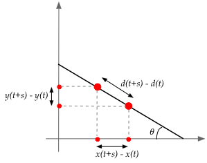
- Consider a bead coming down an incline, as we've seen in our
examples:
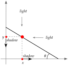
- Suppose we arranged light sources so that shadows of the
bead are projected on the x and y-axes.
- The figure above shows the direction in which the shadows
would move
⇒
Rightwards for the x-axis shadow, downwards for the y-axis shadow.
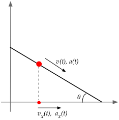
- Suppose we observe only the x-axis shadow:
- The shadow is like a moving object.
- It has a distance, velocity and acceleration functions
that we could measure.
- Similarly, we could observe the y-axis shadow as an
independent object and measure its distance, velocity and
acceleration functions.
Exercise 14:
Execute Incline.java and
observe the shadow objects moving. Are you able to say anything
about whether the shadow objects satisfy our "universal law"?
Next, let's use our incline-simulator to obtain a distance
function along the x-axis:
- The simulator allows you to obtain distance moved by the
x-axis shadow at any time.
- Here's how we'd use it:
(source file)
public class InclineSimulatorExample2 {

    public static void main (String[] argv)
    {
        // Make a new instance of the class.
        InclineSimulator sim = new InclineSimulator ();

        // Set mass and angle.
        sim.mass = 1;
        sim.angle = 30;

        // Measure x(t) = distance moved along x-axis.
        Function dist = new Function ("dist");

        for (double t=1; t<=10; t+=1) {
            sim.run (t);
            double x = sim.getX ();
            dist.add (t, x);
        }

        // Display result.
        dist.show ();
    }

}
Exercise 15:
Download and execute the
above code
Then modify to compute the velocity of the x-axis shadow.
What do you observe?
Let's see what we get for the projectile problem:
- Once again, we'll observe the shadows (x and y) of the ball.
- Suppose we track the x-axis shadow as follows:
(source file)
public class ProjectileSimulatorExample2 {

    public static void main (String[] argv)
    {
        // Make a new simulator object.
        ProjectileSimulator proSim = new ProjectileSimulator ();

        // We want to plot d vs. t along x-axis.
        Function dist = new Function ("distance");

        for (double t=0.1; t<=2.3; t+=0.1) {
            // mass=1, angle=37, initVel=20, s=0.01
            proSim.run (1, 37, 20, t, 0.01);
            // After the simulation is run, get the final x-value.
            double x = proSim.getX ();
            dist.add (t, x);
        }

        // Display.
        dist.show ();
    }

}
Exercise 16:
Execute the above program. What do you notice about the distance
function for the x-axis shadow? Can you explain?
Modify the above code
to estimate and plot velocity. What do you observe?
Exercise 17:
Modify the above code to compute and display the distance and velocity
functions for the y-axis shadow. Do the x-axis and y-axis shadows satisfy
our "universal law"?
Reconstructing motion using "laws along x and y":
Exercise 19:
Explain how \(d(t)\) is estimated in the above code? That is,
why does
d = d + distance (x,y, nextX, nextY);
work? Why did we need the variables nextX, nextY?
Can we similarly construct an \((x,y)\) version for the incline problem?
- First, let's look at the current version of the
simulator for the incline problem:
(source file)
public class InclineSimulator {

    // ... stuff left out (not shown) ...

    public double run (double stopTime)
    {
        // ... initialization not shown ...

	while (true) {
	    // Update time.
	    t += delT;

            // Increase velocity accordingly.
	    v = v + delT * a;

            // Increase distance according to velocity.
            d = d + delT * v;

	    if (t >= stopTime) {
                break;
	    }
	}

        return d;
    }

}
Note:
- This version merely updates \(v(t)\) and \(d(t)\) as
we would expect.
- Recall: \(d(t)\) is distance moved along the incline.
- Keep in mind that \(a(t) = a\) is fixed (constant).
⇒
When \(\theta = 30^\circ\), it turns out that \(a =
4.9\).
(Why this is so will become clear later)
- OK, now let's look an alternative way to write the
incline-simulator:
(source file)
public class InclineSimulatorXY {

    // Mass and angle.
    public double mass = 1;
    public double angle = 30;

    // Separate acceleration, velocity and distance for x and y shadows.
    double ax = 0, ay = 0;
    double vx = 0, vy = 0;
    double x = 0, y = 0;

    // Time and time-step.
    double t = 0;
    double delT = 0.001;

    // Vertical acceleration.
    double g = 9.8;


    public double run (double stopTime)
    {
        // Acceleration along incline: g*sin(inclineangle).
        double angleRadians = 2*Math.PI*angle / 360.0;
        double a = g * Math.sin(angleRadians);

	// Initialize variables.
        vx = 0;  vy = 0;
        x = 0;  y = 0;
        t = 0;

        // We'll track total distance traveled along incline.
        double d = 0;

	while (true) {
	    // Update time.
	    t += delT;

            // Acceleration along x and y.
            ax = a * Math.cos (angleRadians);
            ay = a * Math.sin (angleRadians);

            // Increase velocity according to appropriate acceleration.
            vx = vx + delT * ax;
            vy = vy - delT * ay;

            // Increase distance in each direction according to appropriate velocity.
            double nextX = x + delT * vx;
            double nextY = y + delT * vy;

            // Update total distance traveled.
            d = d + Math.sqrt ((nextX-x)*(nextX-x) + (nextY-y)*(nextY-y));

            x = nextX;
            y = nextY;

	    if (t >= stopTime) {
                break;
	    }
	}

        return d;
    }

}
Note: observe how the appropriate variables are computed for the x-shadow:
ax = a * Math.cos (angleRadians);
- We know that the acceleration along the incline is
a (from the previous version of the inclinesimulator).
- Our reasoning showed that acceleration along the x-direction
(for the x-shadow) is \(a_x(t) = a(t) \cos(angle)\).
- Once we know \(a_x(t)\)
⇒
we can compute \(v_x(t)\)
⇒
From which we can compute \(x(t)\) (distance moved along the x-axis).
Exercise 20:
This clean "separation" into x and y shadows appears mystifying.
Do you believe it works? Download and execute
InclineSimulatorExample3.java
to compare the two simulators.
Print out the horizontal and vertical accelerations.
3.5 Some Unfinished Business
What exactly is \(g\)?
- We know that a dropping (or even a tossed) ball
experiences a downward "pull"
⇒
Informally, we refer to this as gravity.
- Our simulations show that the acceleration is constant
and that the constant is \(g = 9.8\).
- We've used this fact in several simulations:
- In BallDropSimulator and BallTossSimulator:
	    // Update time.
	    t += delT;

            // Decrease velocity by downward acceleration.
	    vy = vy - delT * g;

            // Increase distance (y) according to velocity (which will reduce height)
            y = y + delT * vy;
- In ProjectileSimulator:
            // Apply g to vy. Note: vx stays the same.
            vy = vy - g * delT;
The question we've avoided so far: what causes this
acceleration? Why is it constant?
Exercise 21:
What other parameter in the incline problem remains unaddressed?
(So far, it has not played a role.)
Unfinished business relating to the incline problem:
- We saw that there is acceleration in the x-direction.
⇒
What exactly is causing this acceleration? Who's doing the
"pushing" in that direction?
- Why isn't the vertical acceleration simply \(g\)?
Exercise 22:
Do you have answers for the above two questions?
As it turns out they are quite significant.
Other unanswered questions:
- We haven't talked about units. In what units do we get
\(g=9.8\)? What about units for velocity?
- We've all heard the term "force" used in connection with
the laws of motion. How does "force" relate to what we've
discussed?
3.6 Problem Solving
Let's start by asking a few questions about the Ball-Drop problem:
- What is the final velocity when the ball hits the ground after
being dropped from a height of 1000?
- At what height should one drop the ball to get a final
velocity of approximately 200?
- At what time and height is the velocity half the final
velocity (when dropped from a height of 1000)?
Now let's tackle these questions:
- First, we'll start by modifying the simulator to return
the final velocity instead of time:
(source file)
public class BallDropSimulator2 {

    double vy;
    double t;


    public double run (double height)
    {
	// Initialize variables.
        double a = 9.8;

        // We'll use "y" for distance (falling along y-axis) and "vy" for velocity.
        double y = height;
        vy = 0;

        t = 0;
        double delT = 0.001;

	while (true) {
	    // Update time.
	    t += delT;

            // Decrease velocity by downward acceleration.
	    vy = vy - delT * a;

            // Increase distance (y) according to velocity (which will reduce height)
            y = y + delT * vy;

	    if (y <= 0) {   // Stop if it's hit the ground.
                break;
	    }
	}

        return y;
    }


    public double getV ()
    {
        return vy;
    }


    public double getT ()
    {
        return t;
    }

}
Note:
- We've created methods to return the final velocity and
the time at which the ball hits the ground.
- To do this, we've had to make these variables global.
- We've increased the accuracy slightly (from 0.01 to 0.001).
- Now let's write a separate program to use the simulator
and answer the first question:
(source
file)
public class BallDropSimulatorExercise {

    public static void main (String[] argv)
    {
        BallDropSimulator2 sim = new BallDropSimulator2 ();

        // Drop the ball from a height of 1000.
        sim.run (1000);

        // Obtain final velocity and time taken for the fall.
        double finalVelocity = sim.getV ();
        double timeTaken = sim.getT ();

        System.out.println ("finalVelocity=" + finalVelocity + " time=" + timeTaken);
    }

}
- Recall the second question:
at what height should one drop the ball to get a final
velocity of approximately 200?
- To answer this question, we will try different height
values systematically:
(source
file)
public class BallDropSimulatorExercise2 {

    public static void main (String[] argv)
    {
        BallDropSimulator2 sim = new BallDropSimulator2 ();

        // Drop the ball from a height of 1000.
        double height = 1000;
        sim.run (height);

        double finalVelocity = sim.getV ();

        while ( Math.abs (finalVelocity + 200) > 1 ) {
            // Try different heights systematically.
            height += 1;
            sim.run (height);
            finalVelocity = sim.getV ();
        }

        System.out.println ("Height required: " + height);
    }

}
Note:
- Because velocities are negative (going down), the difference
between the velocity and 200 has a + sign.
Exercise 23:
How many times is the loop iterated?
Can you think of a more efficient algorithm for the same problem?
Exercise 24:
Modify the code to answer the third question:
At what time and height is the velocity half the final
velocity (when dropped from a height of 1000)?
Next, let's look at the ball-tossing problem (toss a ball up
with some initial velocity) and ask these questions:
- What is the maximum height reached by the ball?
- What initial velocity is needed to reach a height of 1000?
- Suppose the ball is launched with an initial velocity
of 50, and suppose we observe the velocity at a height of 100.
Is the velocity the same going up as it is going down at this height?
Let's answer some of these questions now:
- First, we'll modify the simulator to return the velocity:
(source file)
public class BallTossSimulator2 {

    // We made this a global variable ...
    double vy;

    public double run (double stopTime, double initVelocity)
    {
	// Initialize variables.
        double a = 9.8;
        vy = initVelocity;
        double y = 0;
        double t = 0;
        double delT = 0.01;

	while (true) {
	    // Update time.
	    t += delT;

            // Increase velocity accordingly.
	    vy = vy - delT * a;

            // Increase distance according to velocity.
            y = y + delT * vy;

	    if ((t >= stopTime) || (y <= 0)) {
                break;
	    }
	}

        return y;
    }


    public double getV ()
    {
        // ... so that it's accessible here.
        return vy;
    }

}
- Notice the input parameters to the run() method:
- One parameter is the length of the simulation (which might
stop before the ball hits the ground).
- The other is the launch velocity.
- How do we know how much extra time to give (to allow for
the ball to come down and hit the ground)?
⇒
We don't - so let's find out by writing a simple program:
(source file)
public class BallTossExercise {

    public static void main (String[] argv)
    {
        // Make an instance of our new simulator.
        BallTossSimulator2 sim = new BallTossSimulator2 ();

        // We'll start by trying 1 second.
        double stopTime = 1;
        double y = sim.run (stopTime, 50);

        // As long as we haven't hit ground, keep trying higher values of t.
        while (y > 0) {
            stopTime += 10;
            y = sim.run (stopTime, 50);
        }

        // This should be sufficient:
        System.out.println ("stopTime=" + stopTime + " y=" + y);
    }

}
(Turns out: 12 seconds is enough).
- OK, next let's find the maximum height reached:
- How do we do this?
- Here's one idea: we try different stop-time's until,
in two successive attempts, the height decreases.
Here's the program:
(source file)
public class BallTossExercise2 {

    public static void main (String[] argv)
    {
        // Make an instance of our new simulator.
        BallTossSimulator2 sim = new BallTossSimulator2 ();

        // Find the height reached at t=1 and t=2
        double stopTime = 1;
        double prevY = sim.run (stopTime, 50);
        stopTime = 2;
        double nextY = sim.run (stopTime, 50);

        while (nextY > prevY) {
            // As long as y(t+1) > y(t), repeat.
            prevY = sim.run (stopTime, 50);
            stopTime = stopTime + 1;
            nextY = sim.run (stopTime, 50);
        }

        // Now we're sure that y(t+1) < y(t)
        System.out.println ("stopTime=" + stopTime + " prevY=" + prevY + " nextY=" + nextY);
    }

}
- We can add to this code to find the velocity needed to reach
a height of 1000:
(source file)
public class BallTossExercise3 {

    public static void main (String[] argv)
    {
        for (double initVelocity=50; initVelocity<500; initVelocity+=50) {
            // Try this initial velocity:
            double heightReached = getMaxHeight (initVelocity);
            if (heightReached > 1000) {
                // If we've exceeded 1000, then stop.
                System.out.println ("initV=" + initVelocity + "  height=" + heightReached);
                break;
            }
        }
    }


    static double getMaxHeight (double initVelocity)
    {
        // Make an instance of the simulator.
        BallTossSimulator2 sim = new BallTossSimulator2 ();

        // Find the height reached at t=1 and t=2
        double stopTime = 1;
        double prevY = sim.run (stopTime, initVelocity);
        stopTime = 2;
        double nextY = sim.run (stopTime, initVelocity);

        while (nextY > prevY) {
            // As long as y(t+1) > y(t), repeat.
            prevY = sim.run (stopTime, initVelocity);
            stopTime = stopTime + 1;
            nextY = sim.run (stopTime, initVelocity);
        }

        // Now we're sure that y(t+1) < y(t)
        System.out.println ("initV=" + initVelocity + "  stopTime=" + stopTime + " prevY=" + prevY + " nextY=" + nextY);
        return prevY;
    }

}
Note:
- We have made a method out of the sub-problem of "finding
the maximum height for a given initial velocity".
- This sub-problem is then called repeatedly in steps of 50.
Exercise 25:
How would you get a more accurate estimate of the initial
velocity needed to reach 1000?
Next we will address the third question: is
the velocity the same going up and down
at a given height?
- We will first modify the simulator as follows:
- We will stop when a given "target height" is reached.
- We will decide whether this height has been reached
before or after the maximum height has been reached.
- The input parameters now accept the target height, and
whether or not one should reach this target before or after the
maximum:
(source file)
public class BallTossSimulator3 {

    double vy;

    public double run (double stopTime, double initVelocity, double targetHeight, boolean beforeMaxHeight)
    {
	// Initialize variables.
        double a = 9.8;
        vy = initVelocity;
        double y = 0;
        double t = 0;
        double delT = 0.01;

        boolean maxReached = false;

	while (true) {
	    // Update time.
	    t += delT;

            // Increase velocity accordingly.
	    vy = vy - delT * a;

            // Increase distance according to velocity.
            double nextY = y + delT * vy;

            double prevY = y;
            y = nextY;

            if (y < prevY) {
                maxReached = true;
            }

            if (beforeMaxHeight) {
                if (y > targetHeight) {
                    // Done.
                    break;
                }
            }
            else if (maxReached) {
                if (y < targetHeight) {
                    // Done.
                    break;
                }
            }

	    if ((t >= stopTime) || (y <= 0)) {
                break;
	    }
	}

        return y;
    }


    public double getV ()
    {
        return vy;
    }

}
Note:
- We use the same idea (observing successive y values) to see
if the maximum has been reached.
- We wait for "y > target" in the "before" case, and
for "y < target" in the "after" case.
- It's easy now to check the "before" and "after" velocities:
(source file)
public class BallTossExercise4 {

    public static void main (String[] argv)
    {
        // Make an instance of modified simulator.
        BallTossSimulator3 sim = new BallTossSimulator3 ();

        sim.run (1000, 50, 100, true);
        double beforeV = sim.getV ();
        sim.run (1000, 50, 100, false);
        double afterV = sim.getV ();

        System.out.println ("before: " + beforeV + "  after: " + afterV);
    }

}
Exercise 26:
So, is it true that the two velocities are the same?
Is there an intuition for why or why not?
Consider these questions about the projectile problem:
- For a fixed velocity of 50, which angle results in the farthest
horizontal distance traveled?
⇒
This is an age-old ballistics problem
- Suppose we want the projectile to hit a target at a distance
of 200 from the launch point. Find two combinations of angle and
initial velocity to achieve this goal. Of the two, which
one has a smaller time-of-flight?
- We'll begin by re-writing the simulator slightly:
(source file)
public class ProjectileSimulator2 {

    double x=0, y=0;             // Track (x,y)
    double vx, vy;               // Velocity components


    public double run (double angle, double initialVelocity)
    {
        // Initialize values.
        double delT = 0.001;                      // Interval of time.
        double t = 0;                             // Current time.
        double g = 9.8;                           // 9.8 N
        double theta = Math.toRadians (angle);    // Convert degrees to radians.

        x = 0;
        y = 0;

        // Initial vx = component of initialVelocity in x-direction.
        vx = initialVelocity * Math.cos (theta);

        // Initial vy = component of initialVelocity in y-direction.
        vy = initialVelocity * Math.sin (theta);

        while (y >= 0) {
            // Apply g to vy. Note: vx stays the same.
            vy = vy - g * delT;

            // Apply vx to x.
            x = x + vx * delT;

            // Apply vy to y.
            y = y + vy * delT;

            t = t + delT;
        }

        return t;
    }


    public double getX ()
    {
        return x;
    }

}
Note:
- The input parameters are: launch angle and velocity.
- The simulator returns the time taken for the flight.
- There is a method getX() that we can
call to obtain the horizontal distance traveled.
- Next, let's use the initial velocity of 50, and try
different angles:
(source file)
public class ProjectileExercise {

    public static void main (String[] argv)
    {
        // Make an instance of our new simulator.
        ProjectileSimulator2 sim = new ProjectileSimulator2 ();

        // Launch velocity is 50.
        double initV = 50;

        // Try angles in the range [10,80]
        for (double angle=10; angle<=80; angle+=1) {
            sim.run (angle, initV);
            double x = sim.getX ();
            System.out.println ("angle=" + angle + " x=" + x);
        }

    }

}
- A slightly more elegant approach would be to record the
the best result in the loop:
(source file)
public class ProjectileExercise2 {

    public static void main (String[] argv)
    {
        // Make an instance of our new simulator.
        ProjectileSimulator2 sim = new ProjectileSimulator2 ();

        // Launch velocity is 50.
        double initV = 50;

        // Try angles in the range [10,80]
        double bestAngle = 10;
        double bestX = 0;

        for (double angle=10; angle<=80; angle+=1) {
            sim.run (angle, initV);
            double x = sim.getX ();
            if (x > bestX) {
                bestAngle = angle;
                bestX = x;
            }
        }

        System.out.println ("Best angle: " + bestAngle);
    }

}
Exercise 27:
What is the best angle? Run the program and find out.
Does it make intuitive sense?
Exercise 28:
Write code to solve the second problem: find two
angle/velocity combinations to reach a target
at a distance of 200. What is the time-of-flight
for each?
3.7 Problem Solving II
Consider the following problem:
Exercise 29:
Why is it that the route within each region must be
a straight line? Would it be a straight line if there was
an external factor like a strong wind?
Let us draw the configuration on the x-y plane:
- We'll put A on the y-axis, and B on the x-axis:
- Let P be a candidate crossing point.
Exercise 30:
Compute by hand the time taken to go from A to P, and
the time taken to go from P to B in terms of
\(a, b, v_1, v_2, x, y\).
Then download and modify
TwoVelocityProblem.java
and implement your formulas as code. Compare the program's
results with your hand-worked results.
Exercise 31:
Suppose \(v_1\) is (much) smaller than
\(v_2\). Which of the three routes shown
below is likely to be best?
Next, we will start to solve the optimization problem:
- First, some notation:
- \(d_1\) = distance traveled in first phase.
- \(d_2\) = distance traveled in second phase.
- \((a-y)\) = vertical distance in first phase
- \(y\) = vertical distance in second phase
- Since the border is fixed, \(x\) is fixed.
⇒
We only need to find the best possible \(y\) for the
point \(P = (x,y)\).
Exercise 32:
Then download and modify
TwoVelocityProblem2.java
to try different values of \(y\) in a loop.
Next, let's see if we can discover the "law" at work:
- We will vary the ratio \(\frac{v_2}{v_1}\).
- For each possible ratio, we want to identify the
best \(y\) value.
- We would like to discover the relationship between
the ratio \(\frac{v_2}{v_1}\) ... and something
related to the problem parameters.
Exercise 33:
Then download and modify
TwoVelocityProblem3.java
to try different values of \(y\) in a loop, and also
compare with the distances \(d_1, d_2, (a-y),
y\).
Notice that we are using different ratios
\(\frac{v_2}{v_1}\).
- Is there a relationship between \(\frac{v_2}{v_1}\)
and \(\frac{d_2}{d_1}\)?
- Between \(\frac{v_2}{v_1}\)
and the ratio of \((a-y)/d_1\) to \(y/d_2\)?
Now we will consider the case, when velocity is NOT constant:
- Consider a bead sliding down a wire.
- Suppose that we can use two straight-line segments.
- Suppose also that the "kink" doesn't slow down the bead.
Is the fastest way down the straight line (in black)? Or is
it faster to use two segments of different slopes?
- Without loss of generality, we will assume
the starting point is \((x_1,y_1)\)
and that the ending point is \((x_3,y_3)\).
- We are free to choose the "turning" point
\((x_2,y_2)\)
Exercise 34:
Before playing with a simulation, what does your intuition tell you?
We'll start by re-writing our incline simulator to simulate
a single segment:
- A segment will be defined by the end points
\((x_1,y_1)\) (left and above),
and \((x_2,y_2)\) (right and below).
- Here's the code:
(source file)
public class InclineSegmentSimulator {

    // Separate acceleration, velocity and distance for x and y shadows.
    double ax = 0, ay = 0;
    double vx = 0, vy = 0;
    double x = 0, y = 0;

    // Time and time-step.
    double t = 0;
    double delT = 0.001;

    // Vertical acceleration.
    double g = 9.8;


    public double run (double x1, double y1, double x2, double y2, double initvx, double initvy)
    {
        // Acceleration along incline: g*sin(alpha).
        double hyp = distance (x1,y1, x2,y2);
        double xDiff = Math.abs (x1-x2);
        double yDiff = Math.abs (y1-y2);
        double sineOfAngle = xDiff / hyp;
        double cosineOfAngle = yDiff / hyp;

        // Acceleration along incline.
        double a = g * sineOfAngle;

        // Acceleration along x and y.
        ax = a * cosineOfAngle;
        ay = a * sineOfAngle;

	// Initialize velocity components.
        vx = initvx;  vy = initvy;

        // Distance components.
        x = x1;  y = y1;

        t = 0;

	while (true) {
	    // Update time.
	    t += delT;

            // Increase velocity according to appropriate acceleration.
            vx = vx + delT * ax;
            vy = vy - delT * ay;

            // Increase distance in each direction according to appropriate velocity.
            x = x + delT * vx;
            y = y + delT * vy;

	    if ((x > x2) && (y < y2)) {
                // NOTE: this assumes that (x2,y2) is to the right and below.
                break;
	    }
	}

        return t;
    }


    double distance (double x1, double y1, double x2, double y2)
    {
	return Math.sqrt ((x1-x2)*(x1-x2) + (y1-y2)*(y1-y2));
    }


    public double getVx ()
    {
        return vx;
    }


    public double getVy ()
    {
        return vy;
    }

}
Note:
- Compare the calculation of the angle's sine/cosine with your
hand computations.
- Notice that the initial velocity is assumed to be given as input.
- The simulator is written to return the total time taken down
the incline.
- Let's use this simulator as follows for a two-segment problem:
(source file)
public class TwoSegmentIncline {

    public static void main (String[] argv)
    {
        // Make an instance of the simulator.
        InclineSegmentSimulator sim = new InclineSegmentSimulator ();

        // Run the straight incline as one segment.
        double t = sim.run (0, 10, 10, 0, 0, 0);
        System.out.println ("Straight solution: " + t);

        // Now, a potential two segment solution. First segment:
        double t1 = sim.run (0, 10, 5, 5, 0, 0);

        // Get time taken for the second segment:

        double t2 = ...

        // Comparison:
        System.out.println ("Twisted solution: " + (t1+t2));
    }

}
Exercise 35:
Download TwoSegmentIncline.java
and
InclineSegmentSimulator.java
Fill in the missing code above in
InclineSegmentSimulator.
What reasoning did you use in the missing code? What can you
say about the underlying principle?
Next, let's see if we can find a faster two-segment solution:
- Suppose we fix \(x_2 \geq 5\) above (the middle of the incline).
⇒
We will try to find the best \(y_2\).
- One simple way is to try various values:
(source file)
public class TwoSegmentIncline2 {

    public static void main (String[] argv)
    {
        // Make an instance of the simulator.
        InclineSegmentSimulator sim = new InclineSegmentSimulator ();

        // Run the straight incline as one segment.
        double t = sim.run (0, 10, 10, 0, 0, 0);
        System.out.println ("Straight solution: " + t);

        double x2 = 5;
        for (double y2=1; y2<=9; y2+=1) {
            // Now, a potential two segment solution. First segment:
            double t1 = sim.run (0, 10, x2, y2, 0, 0);

            double t2 = ...

            // Comparison:
            System.out.println ("Twisted solution for y2=" + y2 + ": " + (t1+t2));
        }

    }

    // ...

}
Exercise 36:
Fill in the missing code above.
3.8 Summary and an important take-away
We began by stepping into Galileo's shoes to perform some
actual (and messy) experimentation.
Then, we applied Newton's (and, to be fair, Leibniz's) fundamental
insight: if you have an inscrutable function, try taking the
derivative to see if you get insight.
From here, we saw that applying this idea to various
situations (ball drop, toss etc) led to the same observation:
acceleration (2nd derivative of distance) is constant.
This failed for projectile motion:
- When measuring distance along the curve, it does not work.
- However, when we examine the movement of the shadows (which
move along straight lines), it does work.
Thus
- Newton's laws of motion apply to objects moving
in straight lines
- They also apply to the straightline x-and-y shadows of an object moving
in any arbitrary curve.
- The basic trigonometry used to get the
coordinates of the x-y shadows shows that sin/cosine factor out,
making it easy to describe the motion of the shadows.
We were also able to solve standard physics-textbook problems
using our computational approach.
Perhaps the most important take-away is how we perform the
"reverse" of taking derivatives ("integration") computationally:
- We did this by rearranging
$$a(t) \eql \frac{v(t+s) - v(t)}{s}$$
to get
$$v(t+s) \eql v(t) + s \; a(t)$$
- Then, assuming we know the the value at 0, \(v(0) = 0\),
we use the above equation iteratively:
$$\eqb{
v(0 + s) & \eql & v(0) + s \; a(0) \\
v(s + s) & \eql & v(s) + s \; a(s) \\
v(3s) & \eql & v(2s) + s \; a(2s) \\
v(4s) & \eql & v(3s) + s \; a(3s) \\
& \vdots &
}$$
- In a computational loop:
        t = 0;
        v = 0;
        while ( ... )
            t = t + s;
            v = v + s * a;
        }
- Because derivative of distance is velocity, we can "integrate"
velocity in the same way to get distance:
        t = 0;
        v = 0;
        while ( ... )
            t = t + s;
            v = v + s * a;
            d = d + s * v;
        }
Let's revisit this key idea in a little detail.
Exercise 37:
Download and unpack
movingobject.zip.
Then, compile and execute
MovingObject.java.
Examine the code to confirm the basic iteration above.
Observe:
- We see a simple object in motion.
- We are plotting each of distance and velocity against time (two
different curves), when acceleration is fixed.
We will next simplify the code to its most basic form.
Exercise 38:
Write the three lines in the basic iteration to complete
the code in
MovingObjectBasic.java
and then execute to obtain the velocity and distance
curves measured over a shorter span (the first 3 seconds).
Finally, let's tie this to our familiar notion of integration
as "area under the curve".
Exercise 39:
Draw on paper the acceleration function for the range \([0,1]\)
at the points \(0,0.1, 0.2, \ldots,1.0\). The intervals here
are \([0,0.1], [0.1,0.2], \ldots, [0.9,1.0]\).
Calculate the area of each rectangle "under the curve", and
the accumulating sum as you go left to right (so, the area
of the first rectangle, then the area of the first two rectangles,
then the first three etc).
Exercise 40:
Write the one line of code needed to compute the area
of each rectangle in
MovingObjectIntegration.java,
and then compare what you see with your calculations and drawing.
Then, follow the instructions in the program to see the
area accumulation for the velocity curve.
To summarize:
- We finally see that our iteration is nothing but the
area calculation.
- The area is merely calculated by summing up the rectangles
going left to right iteratively.
- Each change going rightwards increases time by \(\Delta t\),
the width of each rectangle.
- The height depends on what function we're integrating.
- The acceleration function in this case was constant (so,
all rectangles have the same height).
⇒
the velocity therefore grows linearly
- Integrating the velocity gives us distance (area under the
velocity curve), which increases non-linearly.
⇒
It turns out to be quadratic.
© 2008, Rahul Simha