The Traveling Salesman Problem (TSP) is possibly the classic
discrete optimization problem.
A preview :
- How is the TSP problem defined?
- What we know about the problem: NP-Completeness.
- The construction heuristics: Nearest-Neighbor, MST,
Clarke-Wright, Christofides.
- K-OPT.
- Simulated annealing and Tabu search.
- The Held-Karp lower bound.
- Lin-Kernighan.
- Lin-Kernighan-Helsgaun.
- Exact methods using integer programming.
Our presentation will pull together material from various sources - see the
references below. But most of it will come from
[Appl2006],
[John1997],
[CS153].
Defining the TSP
The TSP is fairly easy to describe:
- Input: a collection of points (representing cities).
- Goal: find a tour of minimal length.
Length of tour = sum of inter-point distances along tour
- Details:
- Input will be a list of n points, e.g., (x0, y0),
(x1, y1), ..., (xn-1, yn-1).
- Solution space: all possible tours.
- "Cost" of a tour: total length of tour.
→ sum of distances between points along tour
- Goal: find the tour with minimal cost (length).
- Strictly speaking, we have defined the Euclidean TSP.
- There are really three kinds:
- The Euclidean (points on the plane).
- The metric TSP: triangle inequality is satisfied.
- The graph TSP:
Exercise:
- For an n-point problem, what is the size of the solution space
(i.e., how many possible tours are there)?
- What's an example of an instance that's metric but not Euclidean?
Some assumptions and notation for the remainder:
- Let n = |V| = number of vertices.
- Euclidean version, unless otherwise stated.
→
Complete graph.
Some history
Early history:
- 1832: informal description of problem in German handbook for traveling salesmen.
- 1883 U.S. estimate: 200,000 traveling salesmen on the road
- 1850's onwards: circuit judges
Exercise:
Find the following 14 cities in Illinois/Indiana
on a map and identify the best tour you can:
Bloomington, Clinton, Danville, Decatur, Metamora,
Monticello, Mt.Pulaski, Paris, Pekin, Shelbyville,
Springfield, Sullivan, Taylorville, Urbana
- 1960's: Proctor and Gamble $10K competition: a 33-city TSP.
→
Won by a CMU mathematician (and others).
- A related problem: the Knight's tour.
→
Start at bottom-left corner, and visit all squares exactly once and return to the start.
Exercise:
Show how the Knight's tour can be converted into a TSP instance.
- The statisticians take an interest
→
What is the expected length of an optimal tour for uniformly-generated points in 2D?
- Several early analytic estimates in the 1940's.
- Famous Beardwood-Halton-Hammersley result
[Bear1959]:
If L* = optimal tour's length then
L* / √n → a constant
β
- β estimated to be 0.72 for unit-square.
- Human solutions:
- To assess problem-solving skill.
- Part of some neurological tests.
TSP's importance in computer science:
- TSP has played a starring role in the development of algorithms.
- Used as a test case for almost every new (discrete) optimization
algorithm:
- Branch-and-bound.
- Integer and mixed-integer algorithms.
- Local search algorithms.
- Simulated annealing, Tabu, genetic algorithms.
- DNA computing.
Some milestones:
- Best known optimal algorithm: Held-Karp algorithm in 1962, O(n22n).
- Proof of NP-completeness: Richard Karp in 1972
[Karp1972].
→
Reduction from Vertex-Cover (which itself reduces from 3-SAT).
- Two directions for algorithm development:
- Faster exact solution approaches (using linear programming).
→
Largest problem solved optimally: 85,900-city problem (in 2006).
- Effective heuristics.
→
1,904,711-city problem solved within 0.056% of optimal (in 2009)
- Optimal solutions take a long time
→
A 7397-city problem took three years of CPU time.
- Theoretical development:
(let LH = tour-length produced by heuristic,
and let L* be the optimal tour-length)
- 1976: Sahni-Gonzalez result
[Sahn1976].
Unless P=NP no polynomial-time
TSP heuristic can guarantee
LH/L* ≤ 2p(n)
for any fixed polynomial p(n).
- Various bounds on particular heuristics (see below).
- 1992: Arora et al result
[Aror1992].
Unless P=NP, there exists ε>0 such that
no polynomial-time TSP heuristic can guarantee
LH/L* ≤ 1+ε
for all instances satisfying the triangle inequality.
- 1998: Arora result
[Aror1998].
For Euclidean TSP, there is an algorithm that is polyomial for fixed
ε>0 such that
LH/*H ≤ 1+ε
Approximate solutions: nearest neighbor algorithm
Nearest-neighbor heuristic:
- Possibly the simplest to implement.
- Sometimes called Greedy in the literature.
- Algorithm:
     1.   V = {1, ..., n-1}          // Vertices except for 0.
     2.   U = {0}                    // Vertex 0.
     3.   while V not empty
     4.      u = most recently added vertex to U
     5.      Find vertex v in V closest to u
     6.      Add v to U and remove v from V.
     7.   endwhile
     8.   Output vertices in the order they were added to U
Exercise:
What is the solution produced by Nearest-Neighbor
for the following 4-point Euclidean TSP. Is it optimal?
- What we know about Nearest-Neighbor:
-
LH/L* ≤ O(log n)
- There are instances for which
LH/L* = O(log n)
- There are sub-classes of instances for which Nearest-Neighbor
consistently produces the worst tour
[Guti2007].
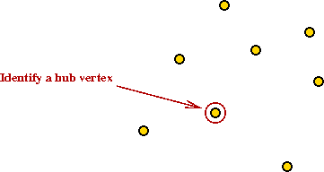
Approximate solutions: the Clarke-Wright heuristic
The Clarke-Wright algorithm:
[Clar1964].
- The idea:
- First identify a "hub" vertex:
- Compute starting cost as cost of going through hub:
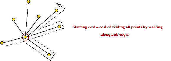
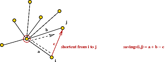
- Identify "savings" for each pair of vertices:
- Take shortcuts and add them to final tour, as long as no
cycles are created.
- Algorithm:
    1.   Identify a hub vertex h
    2.   VH = V - {h}
    3.   for each i,j != h
    4.      compute savings(i,j)
    5.   endfor
    6.   sortlist = Sort vertex pairs in decreasing order of savings
    7.   while |VH| > 2
    8.      try vertex pair (i,j) in sortlist order
    9.      if (i,j) shortcut does not create a cycle
               and degree(v) ≤ 2 for all v
    10.          add (i,j) segment to partial tour
    11.          if degree(i) = 2
    12.             VH =  VH - {i}
    13.          endif
    14.          if degree(j) = 2
    15.             VH =  VH - {j}
    16.          endif
    17.     endif
    18.  endwhile
    19.  Stitch together remaining two vertices and hub into final tour
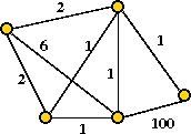
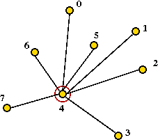
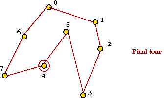
- Example (from above):
- Suppose vertex 4 is the hub vertex:
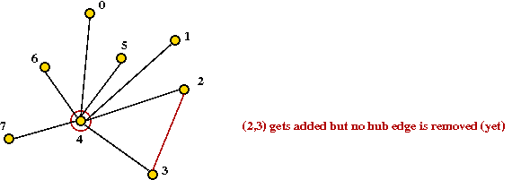
- Suppose (2,3) provides the most savings:
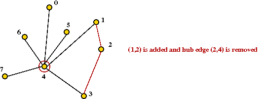
- Next, (1,2) gets added
→
degree(2) = 2
→
must remove hub edge (2,4)
- Continuing ... let's say we obtain:
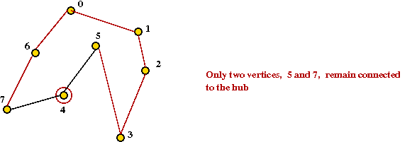
- Finally, add last two vertices and hub into final tour:
- What's known about the CW heuristic:
- Bound is logarithmic:
LH/L* ≤ O(log n)
- Worst examples known:
LH/L* ≥ O(log(n) / loglog(n))
Approximate solutions: the MST heuristic
An approximation algorithm for (Euclidean) TSP that uses the MST:
[Rose1977].
- The algorithm:
- First find the minimum spanning tree (using any MST
algorithm).
- Pick any vertex to be the root of the tree.
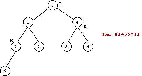
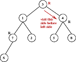
- Traverse the tree in pre-order.
- Return the order of vertices visited in pre-order.
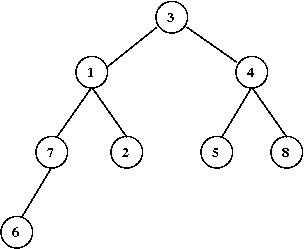
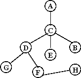
Exercise:
What is the pre-order for this tree (starting at A)?
- Example:
- Consider these 7 points:
- A minimum-spanning tree:
- Pick vertex A as the root:
- Traverse in pre-order:
- Tour:
- Claim: the tour's length is no worse than twice the optimal
tour's length.
What we know about this algorithm:
- The first heuristic to produce solutions within a constant of optimal.
- Easy to implement (since MST can be found efficiently).
Approximate solutions: the Christofides heuristic
The Christofides algorithm:
[Chri1976].
- First, as background, we need to understand two things:
- What is an Euler tour (for general graphs)?
→
A tour that traverses all edges exactly once (but may repeat vertices)
- Famous result: a graph has an Euler tour if and only if all
its vertices have even degree.
- What is a minimal matching for a given subset of vertices V'?
→
A "best" (minimal weight) subset of edges with the property
that no edges have a common vertex
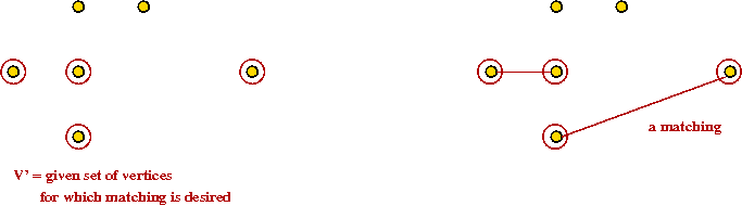
- Important result: min-matching can be found in poly-time.
- The key ideas in the algorithm:
- First find the MST
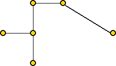
- Then identify the odd-degree vertices
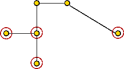
- There are an even number of such odd-degree vertices.
Exercise:
Why?
- Find a minimal matching of these odd-degree vertices and add
those edges
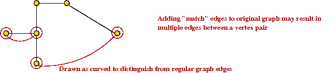
- Now all vertices have even degree.
- Next, find an Euler tour.
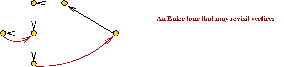
- Now, walk along in Euler tour, but skip visited nodes
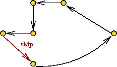
- This produces a TSP tour.
An improved bound:
- We will show that
LH/L* ≤ 1.5
- Let M = cost of MST.
→
L* ≥ M (as argued before).
- Note: we are performing a matching on an even number of vertices.
- Now consider the original odd-degree vertices
- Consider the optimal tour on just these (even # of)
vertices.
- Let LO = cost of this tour.
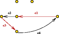
- Let e1, e2, ..., e2k
be the edges.
- Note: E1
= {e1, e3, ..., e2k-1}
is a matching.
- So is E2 =
{e2, e4, ..., e2k}
- Now at least one set has weight at most LO/2.
→
Because both must add up to LO.
- Also the optimal matching found earlier has less weight than
either of these edge sets.
→
min-match-cost ≤ LO/2 ≤ L*/2.
- Thus
min-match-cost + M ≤ L* + L*/2
- But LH uses edges (or shortcuts) from
min-match and MST
→
LH ≤ L* + L*/2
Running time:
- Dominated by O(n3) time for matching.
- Best known matching algorithm: O(n2.376)
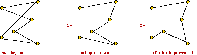
K-OPT
Constructive vs. local-search heuristics:
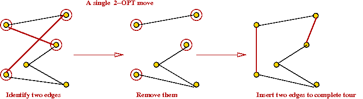
2-OPT:
K-OPT:
- 3-OPT is what you can get by considering replacing 3 edges.
- K-OPT considers K edges.
- Each K-OPT can be time-consuming for K > 3.
What we know about K-OPT:
- For general graphs:
LH/L* ≤ 0.25 n1/2k.
- For Euclidean case,
LH/L* ≤ O(log n).
- In practice: 2-OPT and 3-OPT are much better than the
construction heuristics.
- Note: Any K-OPT move can be reduced to a sequence of 2-OPT moves.
→
But might it might require a long such sequence.
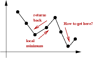
Local Optima and Problem Landscape
Local optima:
- Recall: greedy-local-search generates one state (tour) after
another until no better neighbor can be found
→ does this mean the last one is optimal?
- Observe the trajectory of states:
- There is no guarantee that a greedy local search can find the
(global) minimum.
- The last state found by greedy-local-search is a local minimum.
→ it is the "best" in its neighborhood.
- The global minimum is what we seek: the least-cost
solution overall.
- The particular local minimum found by greedy-local-search
depends on the start state:
Problem landscape:
- Consider TSP using a particular local-search algorithm:
- Suppose we use a graph where the vertices represent states.
- An edge is placed between two "neighbors"
e.g., for a 5-point TSP the neighbors of [0 1 2 3 4] are:
- The cost of each tour is represented as the "weight" of each vertex.
- Thus, a local-search algorithm "wanders" around this graph.
- Picture a 3D surface representing the cost above
the graph.
→ this is the problem landscape for a particular problem and
local-search algorithm.
- A large part of the difficulty in solving combinatorial
optimization problems is the "weirdness" in landscapes
→ landscapes often have very little structure to exploit.
- Unlike continuous optimization problems, local shape in the
landscape does NOT help point towards the global minimum.
Climbing out of local minima:
- A local-search algorithm gets "stuck" in a local minimum.
- One approach: re-run local-search many times with different
starting points.
- Another approach (next): help a local-search algorithm
"climb" out of local minima.
Tabu search
Key ideas:
[Glov1990].
- Suppose we decide to climb out of local minima.
- Danger: could immediately return to same local minima.
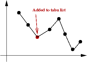
- In tabu-search, you maintain a list of "tabu tours".
→
The algorithm avoids these.
- Each time you pick a minimum in a neighborhood, add that
to the tabu list.
- Various alternatives to tabu-lists
- Always add all neighborhood minimums.
- Only add local minima.
- This way, Tabu forces more searching.
- A problem: a tabu-list can grow very long.
→
Need a policy for removing items, e.g.,
- Least-recently used.
- Throw out high-cost tours.
Simulated annealing
Background:
- What is annealing?
- Annealing is a metallurgic process for improving the
strength of metals.
- Key idea: cool metal slowly during the forging process.
- Example: making bar magnets:
- Wrong way to make a magnet:
- Heat metal bar to high temperature in magnetic field.
- Cool rapidly (quench):
- Right way: cool slowly (anneal)
- Why slow-cooling works:
- At high heat, magnetic dipoles are agitated and move around:

- The magnetic field tries to force alignment:
- If cooled rapidly, alignments tend to be less than optimal
(local alignments):
- With slow-cooling, alignments are closer to optimal (global alignment):

- Summary: slow-cooling helps because it gives molecules more time
to "settle" into a globally optimal configuration.
- Relation between "energy" and "optimality"
- The more aligned, the lower the system "energy".
- If the dipoles are not aligned, some dipoles' fields will conflict
with others.
- If we (loosely) associate this "wasted" conflicting-fields
with energy
→ better alignment is equivalent to lower energy.
- Global minimum = lowest-energy state.
- The Boltzmann Distribution:
- Consider a gas-molecule system (chamber with gas molecules):
- The state of the system is the particular snapshot (positions
of molecules) at any time.
- There are high-energy states:
and low-energy states:
- Suppose the states s1, s2, ...
have energies E(s1), E(s2), ...
- A particular energy value E occurs with probability
P[E] = Z e-E/kT
where Z and k are constants.
- Low-energy states are more probable at low temperatures:
- Consider states s1 and s2
with energies E(s2) > E(s1)
- The ratio of probabilities for these two states is:
r = P[E(s1)] / P[E(s2)]
= e[E(s2) - E(s1)] / kT
= exp ([E(s2) - E(s1)] / kT)
Exercise :
Consider the ratio of probabilities above:
- Question: what happens to r as T increases to infinity?
- Question: what happens to r as T decreases to zero?
What are the implications?
Key ideas in simulated annealing:
[Kirk1983].
- Simulated annealing = a modified local-search.
- Use it to solve a combinatorial optimization problem.
- Associate "energy" with "cost".
→ Goal: find lowest-energy state.
- Recall problem with local-search: gets stuck at local minimum.
- Simulated annealing will allow jumps to higher-cost states.
- If randomly-selected neighbor has lower-cost, jump to it (like
local-search does).
- If randomly-selected neighbor is of higher-cost
→ flip a coin to decide whether to jump to higher-cost state
- Suppose current state is s with cost C(s).
- Suppose randomly-selected neighbor is s' with cost C(s') > C(s).
- Then, jump to it with probability
e -[C(s') - C(s)] / kT
- Decrease coin-flip probability as time goes on:
→ by decreasing temperature T.
- Probability of jumping to higher-cost state depends on cost-difference:
Implementation:
- Pseudocode: (for TSP)
Algorithm: TSPSimulatedAnnealing (points)
Input: array of points

     // Start with any tour, e.g., in input order
1.   s = initial tour 0,1,...,n-1

     // Record initial tour as best so far.
2.   min = cost (s)
3.   minTour = s

     // Pick an initial temperature to allow "mobility"
4.   T = selectInitialTemperature()

     // Iterate "long enough"
5.   for i=1 to large-enough-number
           // Randomly select a neighboring state.
6.         s' = randomNextState (s)
           // If it's better, then jump to it.
7.         if cost(s') < cost(s)
8.             s = s'
               // Record best so far:
9.             if cost(s') < min
10.                min = cost(s')
11.                minTour = s'
12.            endif
13.        else if expCoinFlip (s, s')
               // Jump to s' even if it's worse.
14.            s = s'
15.        endif       // Else stay in current state.
           // Decrease temperature.
16.        T = newTemperature (T)
17.  endfor

18.  return minTour

Output: best tour found by algorithm
Algorithm: randomNextState (s)
Input: a tour s, an array of integers

    // ... Swap a random pair of points ...

Output: a tour
Algorithm: expCoinFlip (s, s')
Input: two states s and s'

1.   p = exp ( -(cost(s') - cost(s)) / T)
2.   u = uniformRandom (0, 1)
3.   if u < p
4.       return true
5.   else
6.       return false

Output: true (if coinFlip resulted in heads) or false
- Implementation for other problems, e.g., BPP
- The only thing that needs to change: define a
nextState method for each new problem.
- Also, some experimentation will be need for the temperature schedule.
Temperature issues:
- Initial temperature:
- Need to pick an initial temperature that will accept large
cost increases (initially).
- One way:
- Guess what the large cost increase might be.
- Pick initial T to make the probability 0.95 (close
to 1).
- Decreasing the temperature:
- We need a temperature schedule.
- Several standard approaches:
- Multiplicative decrease:
Use T = a * T, where a is a constant like 0.99.
→ Tn = an.
- Additive decrease:
Use T = T - a, where a is a constant like 0.0001.
- Inverse-log decrease:
Use T = a / log(n).
- In practice: need to experiment with different temperature
schedules for a particular problem.
Analysis:
- How long do we run simulated annealing?
- Typically, if the temperature is becomes very, very small
there's no point in further execution
→ because probability of escaping a local minimum is miniscule.
- Unlike previous algorithms, there is no fixed running time.
- What can we say theoretically?
- If the inverse-log schedule is used
→ Can prove "probabilistic convergence to global minimum"
→ Loosely, as the number of iterations increase, the
probability of finding the global minimum tends to 1.
In practice:
- Advantages of simulated annealing:
- Simple to implement.
- Does not need much insight into problem structure.
- Can produce reasonable solutions.
- If greedy does well, so will annealing.
- Disadvantages:
- Poor temperature schedule can prevent sufficient exploration
of state space.
- Can require some experimentation before getting it to work well.
- Precautions:
- Always re-run with several (wildly) different starting solutions.
- Always experiment with different temperature schedules.
- Always pick an initial temperature to ensure high probability
of accepting a high-cost jump.
- If possible, try different neighborhood functions.
- Warning:
- Just because it has an appealing origin, simulated annealing
is not guaranteed to work
→ when it works, it's because it explores more of the state
space than a greedy-local-search.
- Simply running greedy-local-search on multiple starting
points may be just as effective, and should be experimented with.
Variations:
- Use greedyNextState instead of the nextState function above.
- Advantage: guaranteed to find local minima.
- Disadvantage: may be difficult or impossible to climb out of
a particular local minimum:
- Suppose we are stuck at state s, a local minimum.
- We probabilistically jump to s', a higher-cost state.
- When in s', we will very likely jump back to
s (unless a better state lies on the "other side").
- Selecting a random next-state is more amenable to exploration.
→ but it may not find local minima easily.
- Hybrid nextState functions:
- Instead of considering the entire neighborhood of 2-swaps,
examine some fraction of the neighborhood.
- Switch between different neighborhood functions during iteration.
- Maintain "tabu" lists:
- To avoid jumping to states already seen before, maintain a
list of "already-visited" states and exclude these from each neighborhood.
- Thermal cycling:
- Periodically raise temperature and perform "re-starts".
- The idea is to force more exploration of the state space.
The Held-Karp lower bound
Our presentation will follow the one in
[Vale1997].
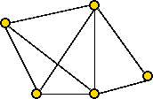
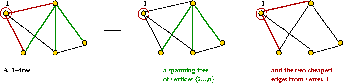
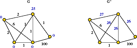
First, a definition:
Held-Karp's idea:
In more detail:
- Let T be a 1-tree and T' be a tour.
- Let dTi =
the degree of node i in T.
- Let L(T,G) = cost of 1-tree T using graph G.
- Let L(T',G) = cost of tour T' using graph G.
- Since every tour is a 1-tree,
minT L(T,G) ≤ minT' L(T',G).
- Now, for a 1-tree T,
L(T,G') = L(T,G) + ΣiεT (diT)πi.
- Similarly, for a tour T',
L(T',G') = L(T',G) + ΣiεT' 2πi.
- Thus, subtracting and taking minimum,
minT L(T,G) +
ΣiεT
(diT-2)πi
≤
minT' L(T',G) = L* (the optimal tour).
- To summarize, we want to find the min-1-tree with weights
π and then correct for that by subtracting off the
additional weights.
- Let W(π) = minT L(T,G) +
ΣiεT
(diT-2)πi.
- Then, the desired "best" Held-Karp bound is:
maxπ W(π).
An optimization procedure:
- Let VT(π) be the vector
(dT1, ..., dTn).
- Let CT(π) be the cost of min-1-tree using π.
- Then, write
W(π) = CT(π) + π VT(π).
- Next, suppose that π' is a vector in
π-space such that
W(π') ≥ W(π).
- Then, Held-Karp show that
(π' - π) VT(π) ≥ 0.
- This means that larger values of W(π') are in the
right half-space pointed to by the vector VT(π).
- Next step: an iterative optimization procedure.
First, a little background on gradient-based optimization:
- Consider a (single-dimensional) function f(x):
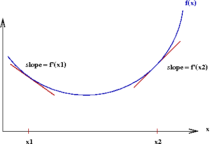
- Let f'(x) denote the derivative of f(x).
- The gradient at a point x is the value of f'(x).
→ Graphically, the slope of the tangent to the curve at x.
- Observe the following:
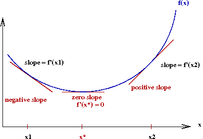
- To the left of the optimal value x*, the gradient
is negative.
- To the right, it's positive.
- We seek an iterative algorithm of the form
     while not over
         if gradient < 0
             move rightwards
         else if gradient > 0
             move leftwards
         else
             stop               // gradient = 0 (unlikely in practice, of course)
         endif
     endwhile
- The gradient descent algorithm is exactly this idea:
     while not over
         x = x - α f'(x)
     endwhile
Here, we add a scaling factor α in case f'(x)
values are of a different order-of-magnitude:
Back to vertex-weight optimization:
- Unfortunately, we don't have a differentiable function.
- For this case, the Russian mathematician Polyak devised
what's called the sub-gradient algorithm:
- For a differentiable function, the gradient "points" in the
right direction.
- For a non-differentiable function, it's still possible to
use a gradient that points in the right direction.
- For the vertex-weights, the iteration turns out to be:
πi(m+1)
=
πi(m) + α(m)
(di - 2).
- Intuitively, this means:
- Increase the weights for vertices with 1-min-tree degree
> 2.
- Decrease the weights for vertices with 1-min-tree degree
< 2.
- Thus, the iteration tries to force the 1-min-tree to be "tour-like".
- Polyak showed that sub-gradient iteration works if the
stepsizes α(m) are chosen properly:
- To summarize:
- Start with some vector of vertex-weights π.
- Repeatedly apply the iteration
πi(m+1)
=
πi(m) + stepsize * sub-gradient VT(π).
- Implementation issues:
- Each iteration requires an MST computation.
→
Can be expensive for large n.
- One approximation: reduce number of edges by considering only
best k neighbors (e.g., k=20).
The Lin-Kernighan algorithm
Key ideas:
- Devised in 1973 by Shen Lin (co-author on BB(N) numbers) and
Brian Kernighan (the "K" of K&R fame).
- Champion TSP heuristic 1973-89.
- LK is iterative:
→
Starts with a tour and repeatedly improves, until no
improvement can be found.
- Idea 1: Make the K edges in K-OPT contiguous
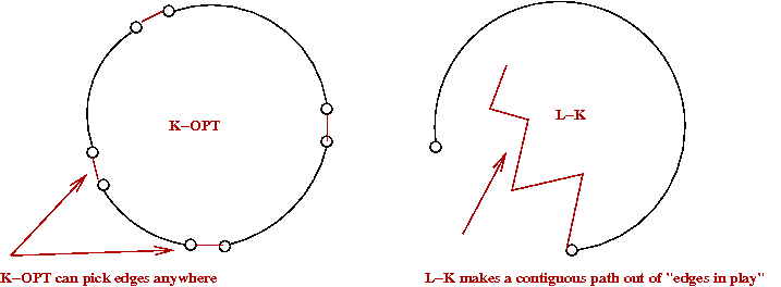
- This is just the high-level idea
→
The algorithm actually alternates between a "current-tour-edge"
and a "new-putative-edge".
- Let the K in K-OPT vary at each iteration.
- Try to increase K gradually at each iteration.
- Pick the best K (the best tour) along the way.
- Allow some limited backtracking.
- Use a tabu-list to create freshness in exploration.
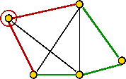
Note: we will use an artificial depiction of a tour as follows:
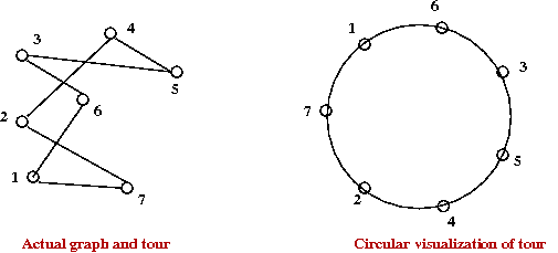
This will be used to explain some ideas.
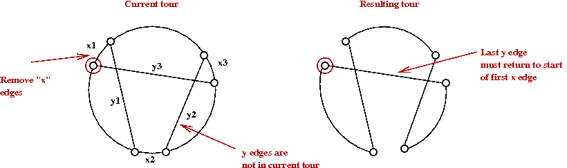
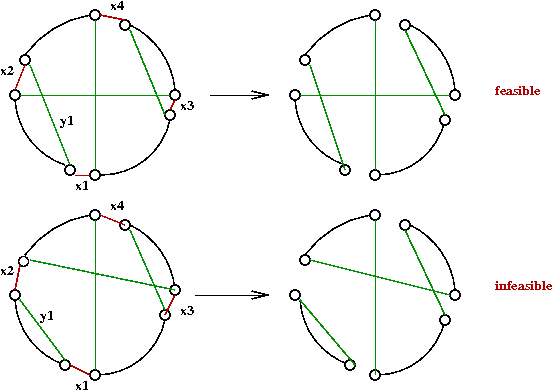
The LK algorithm in more detail:
- At each iteration, LK identifies a sequence of edges
x1, y1,
x2, y2, ...,
xk, yk such that:
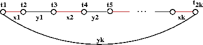
- Each xi is an edge in the current tour.
- Each yi is NOT in the current tour.
- They are all unique (no repetitions).
- The last yk returns to the starting
point t1
- We'll call this an LK-move.
- For example:
- Notice that if we stop at any intermediate
yi, we get a 1-tree.
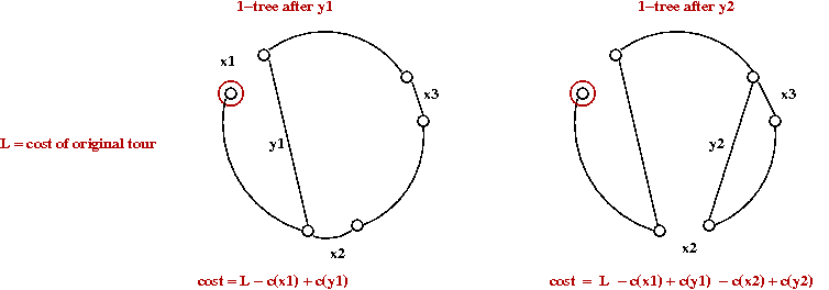
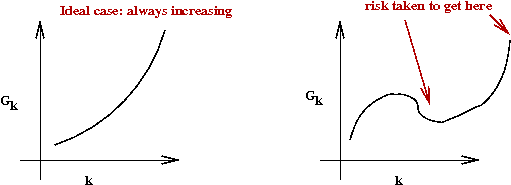
- Let G1 = gain after first x-y-pair:
G1 = c(x1) - c(y1)
- Similarly,
G2 = c(x1) - c(y1)
+ c(x2) - c(y2).
- Gain criterion used by algorithm:
Keep increasing k as long as Gk > 0.
- Note: this is a non-trivial addition because it allows for
a temporary loss in gain:
- Neighbor limitation:
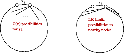
- LK limits the number of neighbors to the m nearest
neighbors, where m is an algorithm parameter (e.g., m=10).
- Re-starts:
- Recall: there are n choices for t1,
the very first node.
- LK tries all n before giving up.
- Best-tour: at all times LK records the best tour found so far.
- Note: LK is actually a little more complicated than
described above, but these are the key ideas.
Performance:
- The standard heuristics (construction, K-OPT) give tours
with 2-5% above Held-Karp.
- LK is usually between 1-2% off.
LKH-1: Lin-Kernighan-Helsgaun
From 1999-2009, Keld Helsgaun
[Hels2009],
added a number of sophisticated optimizations to the basic LK algorithm:
- The first set were added in 1999:
[Hels1999].
→
We'll call this LKH-1.
- And the second set in 2009:
[Hels2009].
→
We'll call this LKH-2.
Key ideas in LKH-1:
- Use K=5 (prefer this value of K over smaller ones).
- Experimental evidence showed that the improvement going from
4- to 5-OPT is much better than 3- to 4-OPT.
- Tradeoff: if K is too high, it takes too long
→
Fewer iterations
→
Less exploration of search space (even if you search a
particular neighborhood more thoroughly).
- Relax sequentiality allow some
xi's and yi's to repeat.
- Replace closest m neighbors with a different
set of M neighbors:
- Problem with LK:
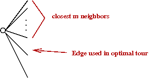
- Recall best 1-tree in Held-Karp bound?
→
Many of these edges are "good" edges for the tour.
→
Experimental evidence: 70-80% of these edges are in optimal tour.
- LKH-1 idea: prefer 1-tree edges that go to neighbors.
- Let L(T) = cost of best 1-tree
→
Can be computed fast (MST)
- For any edge e, let
L(T,e) = cost of best 1-tree that must use e.
- How to force using an edge e?
- Find min-1-tree.
- Add e to tree.
- This causes a cycle.
- Remove heaviest edge in cycle.
- This leaves a min-1-tree that uses e.
- Define &alpha(e) = L(T,e) - L(T) = importance of
e in "1-tree-ness"
- Note: &alpha(e)=0 for any edge in min-1-tree.
- LKH-1 sorts neighbors by α and uses best
m of these.
LKH-2: Lin-Kernighan-Helsgaun, Part 2
Key additions to LKH-1:
- Allow K to increase beyond 5.
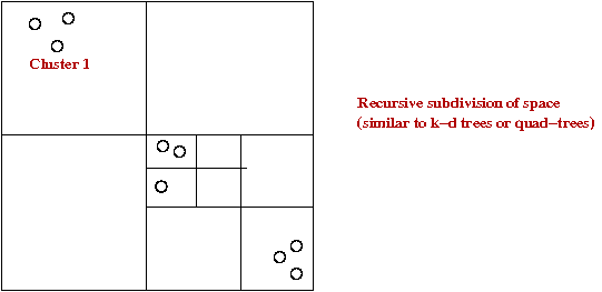
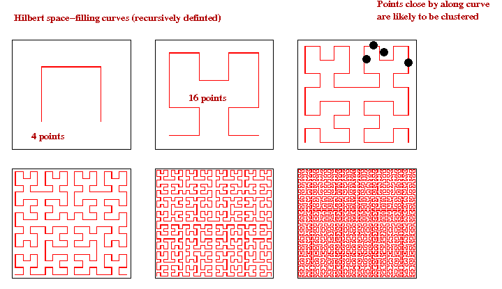
- Problem-partitioning:
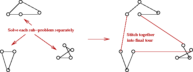
- Divide points into clusters.
- Find best tour for each cluster.
- Stitch together into final tour.
- Run algorithm many times and merge "best parts" from
multiple tours.
→
Called iterative partial transcription.
- Use sophisticated tour data structures to speed up running time.
- Results: million city problem with 0.058% of Held-Karp.
→
Within 0.058% of optimal.
Let's examine the partitioning idea:
Iterative partial transcription (IPT):
- This is an idea from
[Mobi1999].
- Goal: given two tours TA and
TB, compute TC
that is better than both TA and
TB.
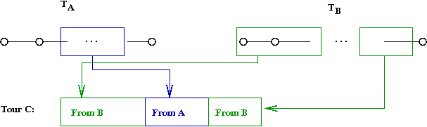
- A single IPT trial-swap between
tours TA and TB
to creates tours
TA' and TB'
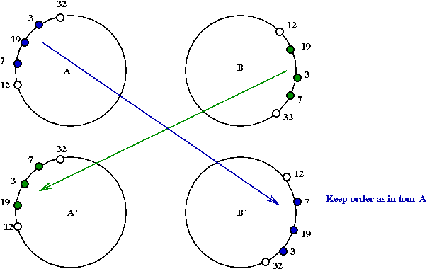
- An IPT-iteration:
- Identifies all possible valid swap segments.
- Tries the swaps and identifies the best possible tour
that can be generated.
- How to use IPT:
- Generate m tours T1, ..., Tm.
- For each pair of tours i,j, perform an IPT-iteration.
Data structures
Given a K-OPT move, is the resulting "tour" a valid tour?
- Example:
- Naive way: walk along new tour T' to see if all vertices are visited
→
O(n) per trial edge-swap
- Another problem: how to maintain tours?
Operations on tour data structures:
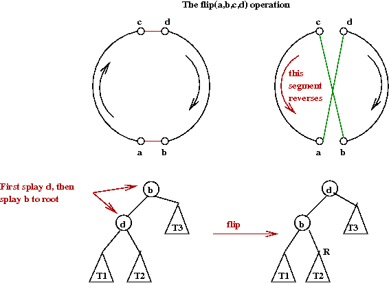
- First, note that any single swap can result in reversing the
tour order for one of the segments affected:
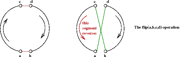
- A single 2-OPT move will be called a flip operation.
- Also, any K-OPT move can be implemented by a sequence of
2-OPT moves.
→
LK-MOVE can be written to use flip operations.
- Other operations that need to be supported:
- next(a): the next node in tour order.
- prev(a): the previous node in tour order.
- between(a,b,c): determine whether b is
between a and c in tour-order.
- Note:
If a flip is performed correctly, it will result in a
valid tour.
- Fredman et al.
[Fred1995]
show a lower bound of (log n) / (loglog n) for these operations.
Arrays:
- Simple to implement.
- But consider what needs to be done to reverse a segment:
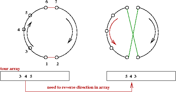
→
Can take O(n).
Doubly-linked lists:
- flip takes O(1) pointer manipulations.
- Order reversal is also easy (comes for free): O(1).
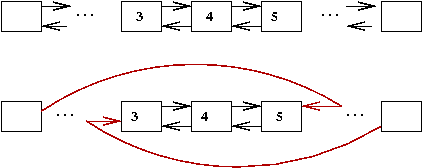
- But finding elements is hard: O(n).
Modified splay trees:
- What is a splay tree?
- Also called a self-adjusting binary tree.
- See
lecture in algorithms course.
- Recall problem with binary trees: can go out of balance.
- Problem with forced balance (e.g. AVL): too much overhead.
→
But use of rotations is useful.
- Example of a splay-step: two mini-rotations:
- Another example:
- In a splay-tree: every accessed node is splayed to the root.
→
Similar to Move-to-Front in linked lists.
- Using a splay-tree for a tour:
- Maintain an external array of pointers into tree, one per node.
- Implementing next(a):
- Recall next(a) in ordinary binary trees: leftmost node of the right subtree.
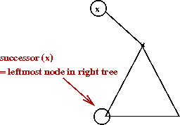
- Locate a using pointer-array: O(1).
- Splay to root.
- Find successor using tour-order (instead of numeric order).
→
With no reversals, this is the leftmost node of the right subtree.
- With reversals, need to change direction for each flip (when recursing).
- The most complex operation is flip():
- Just like the splay-tree, there are several different cases.
- Many involve some type of reversal.
- The general idea (an example):
The segment tree:
- Devised by Applegate and Cook.
- Based on key observation about LK:
- You try a sequence of flips (the LK-move).
- When it doesn't work, you discard the whole sequence.
- In the data structures so far:
- Every flip changes the data structure.
- To discard, we need to undo flips in reverse order.
- A segment-tree tries to avoid the undo part.
- Array representation of tour.
- An auxiliary segment-list:
→
To help with tentative flips.
- An auxiliary segment tree:
→
To help with fast navigation.
Performance:
- Segment-tree is usually best.
- 2-level list is next.
- Splay tree next (with theoretically the best performance).
Exact solution techniques: background
The general idea:
- Formulate TSP as a Integer Programming (IP) problem.
- Apply the cutting-plane approach.
- Judicious choice of cutting-plane heuristics.
But, first, what is Integer Programming? We'll need some
background in linear programming.
Linear programming:
- The word program has different meaning than we are
used to.
→
More like a "programme" of events.
- An LP (Linear Programming) problem is (in standard form):
    max     c1x1 + c2x2 + ... + cnxn
    such that
           a11x1 + ... +  a1nxn ≤ b1
           a21x1 + ... +  a2nxn ≤ b2
           .
           .
           .
           an1x1 + ... +  annxn ≤ bn
    and
           xi ≥ 0,  i=1,...,n
           xi ε R
- In vector/matrix notation:
    max   cTx
    s.t.  Ax ≤ b
           x ≥ 0
- Example:
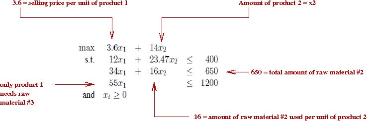
- Geometric intuition of inequality constraints (Ax≤b):
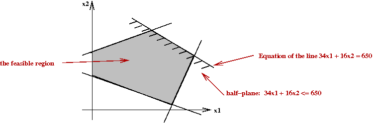
- Each inequality defines a half-plane (half-space).
- The intersection is a polytope (polygon in 2D).
- The feasible region is sometimes called the simplex.
- If we plot objective function "lines":
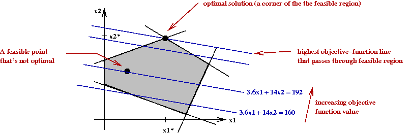
- If we make a line-equation out of the objective function,
some lines will pass through the feasible region.
- Clearly, we want the line with the highest "value" (for a
max problem).
- Sweeping the line upwards (higher value), we want the line
that is the last line to intersect the feasible region.
- This line always intersects the region at a corner.
- Three key algorithms, all major milestones in the
development of LP:
- George Dantzig's Simplex algorithm (1947).
- Leonid Khachiyan's ellipsoid method (1979).
- Narendra Karmarkar's interior-point method (1984).
- The simplex method:
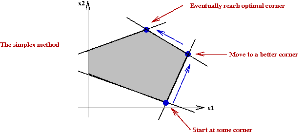
- Start at a corner in the feasible region.
- A simplex-move is a move to a neighboring corner.
- Pick a better neighbor to move to (or even best neighbor).
- Repeat until you've reached optimal solution.
- What's known about the simplex method:
- Guaranteed to find optimal solution.
- Worst-case running time: exponential.
- In practice, it's quite efficient, approximately O(n3).
- Very efficient implementations available, both commercial
and open-source.
- Has been used to solve very large problems (thousands of variables).
- What's known about the other algorithms:
- Khachiyan's ellipsoid method: provably polynomial, but
inefficient in practice.
- Karmarkar's algorithm: provably polynomial and practically
efficient for many types of LP problems.
- Note: an LP problem with equality constraints
    max   cTx
    s.t.  Ax = b
           x ≥ 0
can be converted to an equivalent one in standard form (with
inequality constraints).
- Similarly, a min-problem can be convertex to a max-problem.
Integer programming:
Exact solution techniques: TSP as an IP problem
First, let's express TSP as an IP problem:
- We'll assume the TSP is a Euclidean TSP (the formulation for
a graph-TSP is similar).
- Let the variable xij represent the
directed edge (i,j).
- Let cij = cji = the cost of the
undirected edge (i,j).
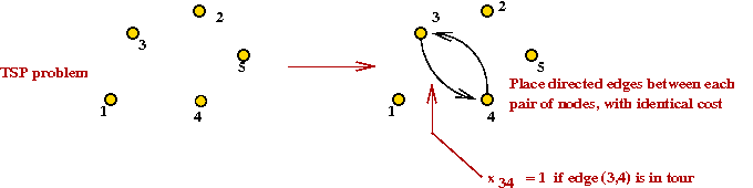
- Consider the following IP problem:
     min    Σi,j  ci,j xi,j
     s.t.    Σj xi,j = 1         // Only one outgoing arc from i
             Σi xi,j = 1         // Only one incoming arc at j
- Unfortunately, this is not sufficient:
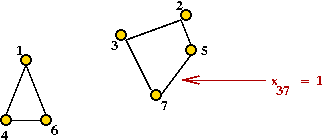
You can get multiple cycles.
→
Called sub-tours
- What to do? Consider this idea:
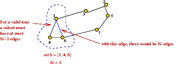
- Consider a subset of vertices S.
- In a valid tour,
Σi,j xi,j ≤ |S|-1
for all i,j ε S.
- This is an inequality constraint that could be added to the
IP problem.
→
Called a sub-tour constraint.
- How many such constraints need to be added to the IP problem?
→
One for each possible subset S.
→
Exponential number of constraints!
- Fortunately, one can add these constraints only as and
when needed (see below).
Solving the IP problem:
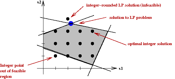
- Naive approach:
- Solve the LP relaxation problem first.
→
Remove integer constraints (temporarily) to get a regular LP, and solve it.
- Round LP solution to nearest integers.
Unfortunately, this may not yield a feasible solution:
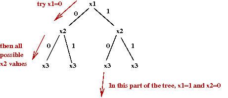
- Branch-and-bound:
- We'll explain this for 0-1-IP problems (variables are binary-valued).
- First, consider a simple exhaustive search, organized
as a tree-search (the "branch" part):
- The tree itself can be explored in a variety of ways:
- Breadth-first (high me
→
High memory requirements.
- Depth-first
→
Low memory requirements.
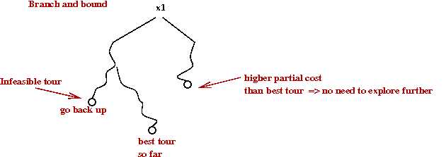
- Cost-first
→
Expand the node that adds the least overall cost to the (partial) objective function.
- Note: if the cost to a node already exceeds the best tour so
far, there's no need to explore further.
→
Parts of the tree can be pruned.
- Cutting planes:
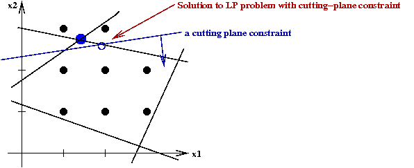
- Add constraints to force the LP-solutions towards integers.
- With a sequence of such constraints, such a process can
converge to an integer solution.
- However, it can take a long time.
- Gomory's algorithm:
- A general cutting-plane algorithm for any IP.
- The idea:
- Solve LP.
- Examine equations satisfied at corner point (of LP).
- Round to integers in inequalities involving those variables.
- Add these to constraints.
- Repeat.
- Unfortunately, it is slow in practice.
History of applying IP to TSP:
- Original cutting plane idea due to Dantzig, Fulkerson and Johnson in 1954.
- Today, there are several families of cutting-plane
constraints for the TSP.
- Branch-and-cut
- Cutting planes "ruled" until 1972.
- Saman Hong (JHU) in 1972 combined cutting-planes with branch-and-bound
→
Called branch-and-cut.
- The idea: some variables might change too slowly with
cutting planes
→
For these, try both 0 and 1 (branch-and-bound idea).
- Alternate way of viewing this:
- More sophisticated "cut" families:
- Grotschel & Padberg, 1970's.
- Padberg and Hong, 1980: 318-city problem.
- Grotschel and Holland, 1987: 666-city problem.
- Padberg and Rinaldi, 1987-88: combined multiple types of
cuts, branch-and-cut and various tricks to solve 2392-city problem.
- During this time, LP techniques improved greatly
→
Can cut down "active" variables in an LP problem.
- Applegate et al (2006)
- Sophisticated LP techniques, new data structures.
- 85,900 city problem.
References and further reading
[WP-1]
Wikipedia entry on TSP.
[WP-1]
Georgia Tech website on TSP.
[Appl2006]
D.L.Applegate, R.E.Bixby, V.Chvatal and W.J.Cook.
The Traveling Salesman Problem, Princeton Univ. Press, 2006.
[Aror1992]
S.Arora, C.Lund, R.Motwani, M.Sudan and M.Szegedy.
Proof verification and hardness of approximation problems.
Proc. Symp. Foundations of Computer Science, 1992, pp.14-23.
[Aror1998]
S.Arora.
Polynomial Time Approximation Schemes for
Euclidean Traveling Salesman and other Geometric Problems.
J.ACM, 45:5, 1998, pp. 753-782.
[Bear1959]
J.Beardwood, J.H.Halton and J.M.Hammersley.
The Shortest Path Through Many Points.
Proc. Cambridge Phil. Soc., 55, 1959, pp.299-327.
[Chan1994]
B.Chandra, H.Karloff and C.Tovey.
New results on the old k-opt algorithm for the
TSP.
5th ACM-SIAM Symp. on Discrete Algorithms, 1994, pp.150-159.
[Clar1964]
G.Clarke and J.W.Wright.
Scheduling of vehicles from a central depot to a number of
delivery points.
Op.Res., 12 ,1964, pp.568-581.
[Chri1976]
N.Christofides.
Worst-case analysis of a new heuristic for the travelling salesman problem.
Report No. 388, GSIA, Carnegie-Mellon University, Pittsburgh, PA, 1976.
[Croe1958]
G.A.Croes.
A method for solving traveling salesman problems.
Op.Res., 6, 1958, pp.791-812.
[Fred1995]
M.L.Fredman, D.S.Johnson, L.A.McGeogh and G.Ostheimer.
Data structures for traveling salesmen.
J.Algorithms, Vol.18, 1995, pp.432-479.
[Glov1990]
F.Glover.
Tabu Search: A Tutorial,
Interfaces, 20:1, 1990, pp.74-94.
[Guti2007]
G.Gutin and A.Yeo.
The Greedy Algorithm for the Symmetric TSP.
Algorithmic Oper. Res., Vol.2, 2007, pp.33--36.
[Held1970]
M.Held and R.M.Karp.
The traveling-salesman problem and minimum spanning
trees.
Op.Res., 18, 1970, pp.1138-1162.
[Hels1998]
K. Helsgaun.
An Effective Implementation of the Lin-Kernighan Traveling Salesman Heuristic,
DATALOGISKE SKRIFTER (Writings on Computer Science), No. 81, 1998,
Roskilde University.
[Hels2009]
K. Helsgaun.
General k-opt submoves for the Lin-Kernighan TSP heuristic.
Mathematical Programming Computation, 2009.
[John1997]
D.S.Johnson and L.A.McGeoch.
The Traveling Salesman Problem: A Case Study in Local Optimization.
In Aarts, E. H. L.; Lenstra, J. K., Local Search in Combinatorial Optimisation, John Wiley and Sons Ltd, pp. 215ˇV310, 1997.
[Karp1972]
R.Karp.
Reducibility among combinatorial problems,
in R. E. Miller and J. W. Thatcher (editors).
, New York: Plenum. pp. 85-103.
[Kirk1983]
S.Kirkpatrick, C.D.Gelatt, and M.P.Vecchi.
Optimization by Simulated Annealing.
Science, 220 1983, pp.671-680.
[Lin1973]
S.Lin and B.W.Kernighan.
An Effective Heuristic Algorithm for the Traveling-
Salesman Problem.
Op.Res., 21, 1973, pp.498-516.
[Mobi1999]
A.Mobius, B.Freisleben, P.Merz and M.Schreiber.
Combinatorial optimization by iterative partial transcription.
Phys.Rev. E, 59:4, 1999, pp.4667-74.
[Rein1991]
G.Reinelt.
TSPLIB ˇX A Traveling Salesman Problem Library.
ORSA J. Comp.,
3:4, 1991, pp. 376-384.
D.J.Rosenkrantz, R.E.Stearns and P.M.Lewis.
An analysis of several heuristics for the traveling salesman
problem.
SIAM J. Computing, Vol.6, 1977, pp.563-581.
[Sahn1976]
S.Sahni and T.Gonzalez. P-complete approximation problems.
J.ACM, Vol.23, 1976, pp.555-565.
[CS153]
R.Simha.
Course notes for CS-153 (Undergraduate algorithms course).
[Vale1997]
C.L.Valenzuela and A.J.Jones.
Estimating the Held-Karp lower bound for the geometric TSP.
European J. Op. Res.,
102:1, 1997, pp.157-175.
Note: The Hilbert curve was an image found on Wiki-commons.