Module objectives
The main goal of this module is to understand Shor's Algorithm,
the landmark breakthrough that launched modern quantum computing.
Along the way, we'll also examine the Quantum Fourier Transform
(QFT) that plays a role in other algorithms.
10.1
Outline: what's needed to understand Shor's algorithm
Shor's algorithm has many parts, each needing different background.
Let's take a quick high-level look at the steps towards
understanding these:
- The mod operator for integers, and greatest common divisor (gcd)
- What is the mod operator, and how does it combine with
regular arithmetic operators?
- What is mod-equivalence, i.e., \(a \equiv_M b\)?
- How does one compute \(\gcd(a,b)\) for integers \(a,b\)?
- Why is the gcd important?
- Why is factoring important and what does it have to do with
breaking cryptography?
- For this purpose we'll look at a summary of how RSA works.
- We'll see that \(M=pq\), for primes \(p\) and \(q\), is the
number we want to factor.
- The order of an integer \(a\) with respect to integer \(M\):
the smallest positive \(r\) such that \(a^r \equiv_M 1\).
- If we can find the order \(r\) that satisfies some properties,
we'll be able to factor \(M\).
- It turns out, we'll need to try different \(a\)'s but not many.
- The Discrete Fourier Transform (DFT):
- What is it, and what does it do?
- How does the DFT help with order-finding?
- The Quantum Fourier Transform (QFT):
- This is a unitary, which will be defined based on the DFT.
- The special (easier) case when the order \(r\) divides
\(N=2^n\) where \(n\) is the number of qubits.
- The more common case when \(r\) does not divide \(N\).
- Finally, implementation: quantum circuits for
order-calculation and QFT.
At this point, it will help to review:
- Appendix A.2:
basic (and simplified) number theory useful as background for Shor's
algorithm.
- Appendix on DFT:
a quick overview of the Discrete Fourier Transform.
10.2
Background: \(\gcd(a,b)\) and its implications
Summary (of Appendix A.2):
- The mod operation gives you the remainder:
\(a \md M\) = the remainder when \(a\) is divided by \(M\).
- Two numbers \(a,b\) are equal modulo-\(M\) if
$$
a \md M \eql b \md M
$$
We will write this written as
$$
a \; \equiv_M \; b
$$
- \(\gcd(a,b)\) = greatest among common divisors of \(a\) and \(b\).
- Euclid's algorithm finds the gcd efficiently.
\(\rhd\)
As much time as the number of digits of the larger number.
- Coprime: \(a\) and \(b\) are coprime if \(\gcd(a,b) = 1\).
10.3
Background: why is factoring important?
Our goal in this section:
- A brief summary of the RSA procedure.
- An example
- A closer look at a few details.
First, the context:
- Most encryption occurs with a secret key:
- Alice and Bob each have a copy of a shared private key.
- This key is used to encrypt a message.
- The actual encryption arithmetic can vary.
- A simple example:
- Suppose \(m\) is the message (a binary string).
- Alice applies
$$
m_e \eql k \oplus m
\;\;\;\; \mbox{\(m_e\) = encrypted bit string}
$$
and sends to Bob.
- Here, \(k\) is the key bitstring.
- Bob receives and applies
$$
m \eql k \oplus m_e
\;\;\;\; \mbox{\(m\) = decrypted bit string}
$$
- Ideally, a secret key is used once and discarded.
- Even if used only a few times, it is challenging for Alice
and Bob to share secret keys.
- Do they do this physically?
- Use some other means?
- Public-key cryptography allows Bob, without any
prior communication with Alice, to send
a message to Alice that only Alice can decode.
- Alice generates two keys, one private and the other public.
- Alice publishes her public-key on her webpage.
\(\rhd\)
Anyone can see the key
- Bob uses that to encrypt a message, and sends it to Alice.
- Alice decodes with her private key.
- We can summarize this Bob-to-Alice communication as:
$$
{\it \mbox{msg}} \eql
{\bf \mbox{Dec}}\parenl{
{\it \mbox{private}}_{\sml{Alice}}, \;
{\bf \mbox{Enc}}({\it \mbox{public}}_{\sml{Alice}}, {\it \mbox{msg}})
}
$$
where
- Bob, who wants to send \({\it msg}\)
downloads \({\it \mbox{public}}_{\sml{Alice}}\)
- Bob computes
$$
m_e \eql
{\bf \mbox{Enc}}({\it \mbox{public}}_{\sml{Alice}}, {\it \mbox{msg}})
$$
- Bob transmits the encrypted message \(m_e\) to Alice
- Alice performs
$$
{\it \mbox{msg}} = {\bf \mbox{Dec}}\parenl{
{\it \mbox{private}}_{\sml{Alice}}, m_e}
$$
- Most often public-key cryptography is used to share
a private key:
- Either Bob makes a secret key, encrypts (via public) and
sends to Alice.
- Or Alice makes one and uses Bob's public key to send.
- There are several public-key schemes, amongst which is the
popular RSA (Rivest-Shamir-Adleman) scheme:
- The public key has two numbers \(e, M\).
- The private key is one number \(d\).
Let's briefly summarize a simplified version of the steps involved
in RSA:
- Alice picks two primes \(p,q\) and computes two numbers
from these:
$$\eqb{
M & \eql & pq
& \;\;\;\;\;\;\mbox{\(M\) is part of the public-key} \\
K & \eql & (p-1)(q-1)
& \;\;\;\;\;\;\mbox{\(K\) is kept secret, used for calculating keys} \\
}$$
- Alice then finds \(e \lt K\) so that
\(e\) is coprime to \(K\).
- Let \(d\) be the unique inverse of \(e\) modulo-\(K\)
$$
d e \; \equiv_{K} \; 1
$$
- Proposition A.2.5
shows why \(d\) exists and is unique.
- Alice publishes \(e\) and \(M\), and keeps everything else secret:
$$\eqb{
\mbox{public key: } & \;\;\;\; & (e, M) \\
\mbox{private key: } & \;\;\;\; & d \\
}$$
- Bob now wishes to send Alice a message.
- Bob downloads \(e\) and \(M\).
(So does Eve the eavesdropper.)
- Let \(m \lt M\) be the integer that Bob wants to
send.
\(\rhd\)
\(m\) is the "message"
- Bob computes
$$\eqb{
m_e & \eql & \mbox{encrypted version of \(m\)} \\
& \eql & m^e \md M
}$$
and sends \(m^e \md M\) to Alice.
- Alice decrypts by computing
$$
(m^e)^d \md M
$$
This turns out to be
$$
(m^e)^d \md M \eql m
$$
And thus Alice receives the message.
- Eve has \(e\) and \(M\).
- If Eve could factor \(M = pq\), she can compute \(K=(p-1)(q-1)\),
and from there easily compute \(d\), the inverse of \(e\)
$$
d e \; \equiv_{K} \; 1
$$
An example:
- Suppose Alice picks primes \(p=41, q=67\).
- Then, she computes
$$\eqb{
M & \eql & pq & \eql & 41 \times 67 & \eql & 2747 \\
K & \eql & (p-1)(q-1) & \eql & 40 \times 66 & \eql & 2640
}$$
- Suppose Alice picks \(e=1013\) so that \(\gcd(e,K)=\gcd(1013,2640)=1\)
\(\rhd\)
That is, \(e\) and \(K\) are coprime.
- She computes the inverse \(d=1277\) so that
$$
de \md K \eql (1277 \times 1013) \md 2640 \eql 1
$$
- Alice publishes \(e=1013, M=2747\).
- Bob wishes to send the message \(m=601\) ("one minute past
0600 hours")
- Note: \(m\) needs to be less than \(M\).
- Long messages (from text) can be broken down into smaller chunks.
- Bob computes
$$\eqb{
m_e & \eql & \mbox{encrypted version of \(m\)} \\
& \eql & m^e \md M \\
& \eql & 601^{1013} \md 2747 \\
& \eql & 998
}$$
and sends \(m_e = 998\), the encrypted message, to Alice.
- Alice decrypts by computing
$$\eqb{
(m^e)^d \md M
& \eql & 998^{1277} \md 2747 \\
& \eql & 601
}$$
and recovers the original message.
Now let's take a closer look:
- Let's now recall the version of the Chinese Remainder
Theorem stated as
Proposition A.2.6,
of the Appendix:
Proposition A.2.6:
Suppose \(x, p, q\) and \(m\) are integers with \(p,q\) coprime,
and that
$$\eqb{
x \md p & \eql & m \\
x \md q & \eql & m \\
}$$
Then
$$
x \md pq \eql m \\
$$
- Thus, to show that
$$
m^{de} \; \equiv_{pq} \; m
$$
it is sufficient to show both
$$\eqb{
m^{de} & \; \equiv_{p} \; & m\\
m^{de} & \; \equiv_{q} \; & m
}$$
- We'll do this for \(p\). The same reasoning applies to \(q\).
- First, let's state Fermat's Little Theorem, proved
as Proposition A.2.7
in the Appendix:
Proposition A.2.7: (Fermat's Little Theorem)
If \(p\) is a prime then
$$
a^{p-1} \; \equiv_p \; 1
$$
for any positive integer \(a\) that is not a multiple of \(p\).
- Now, returning to RSA:
- Since \(de \equiv_K 1\), let \(s\) be the multiplier so that
$$
de \eql sK + 1 \eql s(p-1)(q-1) + 1
$$
for some \(s\).
- Then,
$$\eqb{
m^{de} & \eql & m^{s(p-1)(q-1) + 1} \\
& \eql & m \left( m^{s(q-1)} \right)^{p-1}
}$$
- Now, if \(m\) is a multiple of \(p\)
$$
m^{de} \; \equiv_{p} 0
$$
But \(m \equiv_p 0\) too. And hence, for this case
$$
m^{de} \; \equiv_{p} m
$$
- Next, suppose \(m\) is not a multiple of \(p\), then we can
apply Fermat's Little Theorem to \(a=m^{s(q-1)}\) and conclude that
$$
m^{s(q-1)} \; \equiv_p \; 1
$$
Which means that
$$
m m^{s(q-1)} \; \equiv_p \; m
$$
- Thus, for the case \(m\) is not a multiple of \(p\),
$$
m^{de} \; \equiv_{p} m
$$
- The same arguments apply to \(q\), and so, we've shown
$$\eqb{
m^{de} & \; \equiv_{p} \; & m\\
m^{de} & \; \equiv_{q} \; & m
}$$
- Which means
$$
m^{de} \; \equiv_{pq} \; m
$$
as desired.
- What remains is to know that modular exponentiation
like \(m^e \md M\) can be performed efficiently:
- First observe that if \(e=2^k\) (any power of 2), then
\(k\) successive doublings can compute \(e\).
\(\rhd\)
This is efficient
- Any other \(e\) can be written in terms of powers-of-2
$$
e \eql e_{n-1}2^{n-1} + e_{n-2}2^{n-2} + \ldots + e_02^{0}
$$
via its binary expansion.
- Each term in the sum can be computed by successive doubling,
and there are only as many terms as the number of binary digits.
\(\rhd\)
This too is efficient
- We also need to show that the inverse \(d\) of \(e\)
can be computed efficiently:
- This is done using an extension of Euclid's algorithm,
as shown in the section on Bezout's lemma,
Proposition A.2.1,
of the Appendix.
Note: everything so far is classical. Nothing quantum yet.
10.4
Background: order-finding and its relationship to factoring
Let's start with some definitions:
Order-finding and factoring:
- Recall: if \(f_{a,M}(x)\) has order \(r\), then
\(r\) is the smallest integer such that
$$
f_{a,M}(r) \eql 1
$$
That is,
$$
a^r \; \equiv_M \; 1
$$
- The condition \(a^r \md M = 1\) implies
$$
a^r - 1 \; \equiv_M \; 0
$$
- Suppose \(r\) is even.
- Then \(\frac{r}{2}\) is an integer.
- We can factor
$$
a^r - 1 \eql (a^{\frac{r}{2}} + 1)(a^{\frac{r}{2}} - 1)
$$
- And so
$$
(a^{\frac{r}{2}} + 1)(a^{\frac{r}{2}} - 1) \; \equiv_M \; 0
$$
- Next, we cannot have
$$
(a^{\frac{r}{2}} - 1) \; \equiv_M \; 0
$$
- This would imply \(a^{\frac{r}{2}} \; \equiv_M \; 1\),
contradicting the fact that \(r\) is the smallest such that
\(a^r \; \equiv_M \; 1\).
- Thus, \(a^{\frac{r}{2}} - 1\) is not a multiple of \(M=pq\).
- Suppose that \(a^{\frac{r}{2}} + 1 \equiv_M 0\)
happens to be false:
- That is, \(a^{\frac{r}{2}} + 1\) is also not a multiple of \(M=pq\).
- Then, neither \(a^{\frac{r}{2}} + 1\) nor \(a^{\frac{r}{2}} - 1\)
is a multiple of \(pq\) but their product is:
$$
(a^{\frac{r}{2}} + 1)(a^{\frac{r}{2}} - 1) \; \equiv_M \; 0
$$
- This can happen if one of \(p\) or \(q\) divides
\(a^{\frac{r}{2}} + 1\) and the other divides \(a^{\frac{r}{2}} - 1\).
- For example:
$$\eqb{
a^{\frac{r}{2}} + 1 & \eql & k_1 p \\
a^{\frac{r}{2}} - 1 & \eql & k_2 q \\
}$$
Then,
$$
(a^{\frac{r}{2}} + 1)(a^{\frac{r}{2}} - 1)
\eql k_1 k_2 pq
$$
- If this situation holds, it must be that
$$
\gcd \parenl{M, a^{\frac{r}{2}} + 1} \eql p
$$
because:
- \(p\) and \(q\) are the only divisors of \(M\).
- And \(p\) (but not \(q\)) is a divisor of \(a^{\frac{r}{2}} + 1\).
- Since we don't know whether \(p\) divides
\(a^{\frac{r}{2}} + 1\) or \(a^{\frac{r}{2}} - 1\),
we try both:
$$\eqb{
p & \eql & \gcd \parenl{M, a^{\frac{r}{2}} + 1}? \\
p & \eql & \gcd \parenl{M, a^{\frac{r}{2}} - 1}? \\
}$$
If we get one (say, \(p\)), the other is obtained from \(M=pq\).
- All of the above depended on being lucky that
\(a^{\frac{r}{2}} + 1 \equiv_M 0\) happens to be false, based on \(a\).
- A bit more advanced number theory shows that this
occurs with probability at least 0.5
- Which means a few repeated trials with different \(a\)'s should
be enough.
To summarize:
- Given \(M\), and some \(a\) such that \(\gcd(a,M)=1\),
the order \(r\) is:
$$
r \eql \mbox{the smallest positive integer \(x\) such that \(a^x \md M = 1\)}
$$
- Once we know \(r\), we can factor \(M=pq\) if \(a\) is lucky
for us in two ways:
- \(\frac{r}{2}\) is an integer (\(r\) is even)
\(\rhd\)
Probability = \(0.5\)
- \(a^{\frac{r}{2}} + 1 \equiv_M 0\) is false
\(\rhd\)
Probability much higher than \(0.5\)
- If not, we simply try different values of \(a\).
- The probability of satisfying both is at least 0.25
- The probability of being repeatedly unlucky falls off
exponentially.
Thus, once we have the order \(r\) for some \(a\), then \(M=pq\)
can be factored efficiently.
- Finally, we should ask: can the order \(r\) be
classically computed in an efficient manner?
- The current belief is: no
- Because if one could do that, factoring could be done
efficiently, as we've seen.
- At least, this is the premise of (classical) cryptography.
- Shor's algorithm, on the other hand, shows how a quantum
approach can perform order-finding efficiently.
10.5
Background: the DFT and QFT
Assumed background: Appendix on DFT
- The N-th roots of \(1\).
- \(\wn\), one of these N-th roots.
- Construction of the DFT matrix using powers of \(\wn\).
- What the matrix does to a vector.
For now, let's summarize:
- Note: we will use the unitary version:
$$
U_{\smb{DFT}}
\eql
\frac{1}{\sqrt{N}}
\mat{
1 & 1 & 1 & \ldots & 1 \\
1 & w & w^2 & \ldots & w^{N-1} \\
1 & w^2 & w^4 & \ldots & w^{2(N-1)} \\
1 & w^3 & w^6 & \ldots & w^{3(N-1)} \\
\vdots & \vdots & \vdots & \vdots & \vdots \\
1 & w^k & (w^k)^2 & \ldots & w^{k(N-1)} \\
\vdots & \vdots & \vdots & \vdots & \vdots \\
1 & w^{N-1} & w^{2(N-1)} & \ldots & w^{(N-1)(N-1)}
}
$$
- At its most basic, the Discrete Fourier Transform is
a matrix designed to transform one set of coordinates into
another:
- Thus, if \(\kt{v}=(a_0,\ldots,a_N)\) is a vector, then
$$
\tilde{v} \eql U_{\smb{DFT}} \kt{v}
$$
can be expanded as
$$
\kt{\tilde{v}}
\eql
\mat{ \tilde{a}_0 \\ \tilde{a}_1 \\ \tilde{a}_2\\ \vdots \\ \tilde{a}_{N-1} }
\eql
\mat{
1 & 1 & 1 & \ldots & 1 \\
1 & w & w^2 & \ldots & w^{N-1} \\
1 & w^2 & w^4 & \ldots & w^{2(N-1)} \\
1 & w^3 & w^6 & \ldots & w^{3(N-1)} \\
\vdots & \vdots & \vdots & \vdots & \vdots \\
1 & w^k & (w^k)^2 & \ldots & w^{k(N-1)} \\
\vdots & \vdots & \vdots & \vdots & \vdots \\
1 & w^{N-1} & w^{2(N-1)} & \ldots & w^{(N-1)(N-1)}
}
\mat{ a_0 \\ a_1 \\ a_2 \\ \vdots \\ a_{N-1} }
$$
- We will think of \( U_{\smb{DFT}}\) as
an operator acting on \(\kt{v}\) to produce \(\tilde{v}\).
- Because \( U_{\smb{DFT}}\) is unitary, it is a valid
quantum unitary transformation, which we will henceforth write
as \( U_{\smb{QFT}}\)
- It will be convenient to write the transformation
algebraically:
$$
\kt{\tilde{v}}
\eql U_{\smb{QFT}} \kt{v}
\eql
\smf{1}{\sqrt{N}} \sum_{y=0}^{N-1} \sum_{x=0}^{N-1}
a_x w^{xy} \kt{y}
$$
- We've seen that \(U_{\smb{QFT}}\) has the ability to
extract periodicity in data.
- Since the order function \(f_{a,M}\) is periodic with
period \(r\), this suggests that the \(U_{\smb{QFT}}\) could
help in discovering \(r\).
- And knowing \(r\), as shown earlier, leads to factoring.
- Finally, we'll expand \(w=e^{ \frac{2\pi i}{N} }\)
in the above expression:
$$
U_{\smb{QFT}} \kt{v}
\eql
\smf{1}{\sqrt{N}} \sum_{y=0}^{N-1} \sum_{x=0}^{N-1}
a_x e^{ \frac{2\pi xy i}{N} } \kt{y}
$$
This is to highlight the following:
- The amplitudes (coefficients) of the \(\kt{y}\)'s
are being modified by \(e^{ \frac{2\pi xy i}{N} }\).
- The modification is a relative-phase modification.
In-Class Exercise 1:
Suppose \(\kt{v}\) is the standard basis vector \(\kt{x}\)
for some integer \(x\).
What is the result of applying \(U_{\smb{QFT}}\) to \(\kt{x}\)?
10.6
A first step towards order-finding (that almost works)
Suppose we have a quantum circuit \(U_f\) that computes \(f_{a,M}(x)\)
for input \(x\) where
$$
f_{a,M}(x) \eql a^x \md M
$$
- That is, the circuit does not find the order (the smallest
such \(x\) that \(a^x \md M = 1\)).
\(\rhd\)
It simply computes \(a^x \md M\).
- Also, to simplify notation, let's assume \(a\) and \(M\)
are understood and write
$$
f(x) \eql a^x \md M
$$
This produces an integer, which means it can be written as
a standard-basis vector.
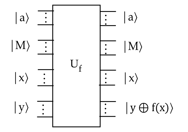
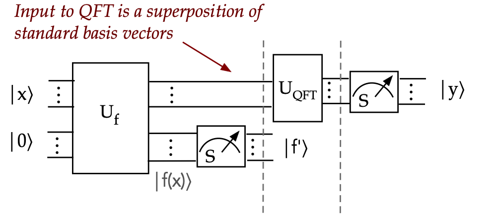
- Let's draw the circuit as:

- We will simplify the figure to focus on the input
\(x\) and function output \(\kt{y\oplus f(x)}\):

Note:
- The assumption here is that \(a,M\) are still inputs but just
not shown in the figure.
- We'll assume \(n\)-qubit input \(\kt{x}\)
- And \(n\)-qubit output
$$
U_f \kt{x}\kt{y} \eql \kt{x}\kt{y\oplus f(x)}
$$
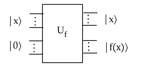
- Setting \(\kt{y}=\kt{0}\) as usual, the output qubits hold
\(\kt{f(x)}\):
$$
U_f \kt{x}\kt{0} \eql \kt{x}\kt{f(x)}
$$
where
\(f(x) \eql a^x \md M\).
- Remember, \(\kt{f(x)}\) is a standard-basis vector.
- Now, let's apply the usual equal-superposition input:
$$
U_f \smf{1}{\sqrt{N}} \sum_x \kt{x}\kt{0}
\eql \smf{1}{\sqrt{N}} \sum_x U_f \kt{x}\kt{0}
\eql \smf{1}{\sqrt{N}} \sum_x \kt{x}\kt{f(x)}
$$
- At this point, we merely have an (entangled) association of each
\(\kt{x}\) with its corresponding \(\kt{f(x)}\).
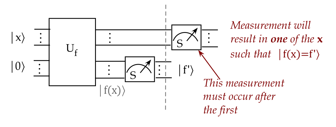
- Now for a key insight: suppose we measure only the
second \(n\) qubits:

- The measurement will result in some standard-basis
vector \(\kt{f^\prime}\).
- However, recall that \(f(x)\) repeats:
- There are many \(\kt{x}\)'s that map to the same \(\kt{f^\prime}\).
- All of these will be present as a superposition
in the upper \(n\) qubits.
- To see how this occurs, let's revisit the example from Module 10:
- Consider this 2-qubit state:
$$
\ksi \eql \kt{a}\kt{0} + \kt{b}\kt{0} + \kt{c}\kt{1} + \kt{d}\kt{1}
$$
If we measure the second qubit and obtain \(\kt{0}\), we know
the 2-qubit outcome is:
$$
\kt{a}\kt{0} + \kt{b}\kt{0} \eql (\kt{a} + \kt{b})\kt{0}
$$
Which creates a 1st-qubit superposition.
- Returning to our problem, suppose there are \(m\) values of \(x\),
call them \(x_0,\ldots,x_{m-1}\) such that
$$
f(x_i) \eql f^\prime
$$
- Then, the complete output after measurement will be
this superposition in the first \(n\) qubits:
$$
C \sum_{i=0}^m \kt{x_i} \kt{f^\prime}
$$
where \(C\) normalizes for unit-length: \(C = \frac{1}{\sqrt{m}}\).
Let's look at an example:
- Consider \(M=15, a=7\)
- Then
$$
f(x) \eql f_{a,M}(x) \eql a^x \md M \eql 7^x \md 15
$$
- Suppose we happen to see \(f^\prime = 13\):
- Which \(x\)'s correspond to \( f(x) = 13\)?
- Let's now try different \(x\) and see:
$$
\begin{array}{|c|c|}\hline
x & 7^x \md 15 & f^\prime\\\hline
0 & 1 & \\
1 & 7 & \\
2 & 4 & \\
3 & 13 & f^\prime=13\\
{\bf 4} & {\bf 1} & \\
5 & 7 & \\
6 & 4 & \\
7 & 13 & f^\prime=13 \\
8 & 1 & \\
9 & 7 & \\
10 & 4 & \\
11 & 13 & f^\prime=13 \\
12 & 1 & \\
13 & 7 & \\
14 & 4 & \\
15 & 13 & f^\prime=13 \\
\vdots & \vdots & \\
30 & 4 & \\
31 & 13 & f^\prime=13\\
\hline
\end{array}
$$
Here:
- We see that \(r=4\), meaning \(r=4\) is the smallest positive
integer for which \(a^r\md M = 1\).
- Because \(f\) repeats with period \(r=4\), the \(x\) values
that result in \(f(x)=13\) are:
$$
x \in \setl{ 3, 7, 11, \ldots, 31}
$$
- In general, for any output value \(f^\prime\), let
\(x_{f^\prime}\) be the smallest \(x\) such that \(f(x_{f^\prime})
= f^\prime\)
- When \(f^\prime=13\) above, the first \(x\) to give this is
\(x_{f^\prime} = 3\)
- We can think of \(x_{f^\prime}\) as the offset from where
the periodicity begins.
- Then we can describe all the values resulting in
\(f^\prime\) as \(x_{f^\prime} + kr\), for \(k=0,1,2,\ldots\):
$$\eqb{
k=0 & \; \Rightarrow \; &
x_{f^\prime} + kr & \eql & 3 + 0 \times 4 & \eql & 3 & \mbx{First value} \\
k=1 & \; \Rightarrow \; &
x_{f^\prime} + kr & \eql & 3 + 1 \times 4 & \eql & 7 & \mbx{Second value} \\
k=2 & \; \Rightarrow \; &
x_{f^\prime} + kr & \eql & 3 + 2\times 4 & \eql & 11 & \mbx{Third} \\
\vdots & & & & & \\
}$$
- The output after applying \(U_f\) before measurement
is
$$
U_f \sum_x \kt{x}\kt{0} \eql \sum_x U_f \kt{x}\kt{0}
\eql \sum_x \kt{x}\kt{f(x)}
$$
where we've left out \(\frac{1}{\sqrt{N}}\) to avoid clutter below.
- In our example, that is
$$\eqb{
& \; & \kt{0}\kt{f(0)} \, + \, \kt{1}\kt{f(1)} \, + \, \kt{2}\kt{f(2)}
\, + \, \kt{3}\kt{f(3)} \\
& \; & + \kt{4}\kt{f(4)} \, + \, \kt{5}\kt{f(5)} \, + \, \kt{6}\kt{f(6)}
\, + \, \kt{7}{f(7)}\\
& \; & + \ldots + \kt{30}\kt{f(31)} \, + \, \kt{31}\kt{f(32)} \\
& \eql &
\kt{0}\kt{1} \, + \, \kt{1}\kt{7} \, + \, \kt{2}\kt{4}
\, + \, {\bf \kt{3}\kt{13}} \\
& \; & + \kt{4}\kt{1} \, + \, \kt{5}\kt{7} \, + \, \kt{6}\kt{4}
\, + \, {\bf \kt{7}\kt{13}}\\
& \; & + \ldots + \kt{30}\kt{4} \, + \, {\bf \kt{31}\kt{13}}
}$$
- When we measure the output qubits, we get some particular
\(f^\prime\), for example, \(f^\prime=13\), only those terms
in the output superposition with \(f^\prime=13\) will remain:
$$
{\bf \kt{3}\kt{13}} + {\bf \kt{7}\kt{13}} + \ldots + {\bf \kt{31}\kt{13}}
$$
Which means the output can be factored as
$$
\parenl{ \kt{3} + \kt{7} + \ldots + \kt{31} } \, \kt{13}
$$
- And because they had equal weight as input, they will have
equal weight as output.
- If there are \(m\) such terms, then the output is
$$
C \sum_{k=0}^{m-1} \kt{3 + kr} \kt{13}
$$
where \(C\) is the normalizing constant (and \(3\) is the offset).
- Note: because this is an equal superposition with
\(m\) terms, \(C = \frac{1}{\sqrt{m}}\).
- Thus, the output is
$$
\smf{1}{\sqrt{m}} \sum_{k=0}^{m-1} \kt{x_{f^\prime} + kr} \kt{f^\prime}
$$
- Now for the key observation: the top qubits contain
\(r\)!
At this point, we are getting close to identifying \(r\):
10.7
A second step towards order-finding (that almost works)
The one thing we do know about the top qubits after the first
measurement: there is periodicity involving \(r\):
$$
\smf{1}{\sqrt{m}} \sum_{k=0}^{m-1} \kt{x_{f^\prime} + kr} \kt{f^\prime}
$$
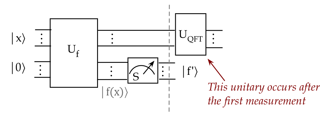
The obvious question is: could the periodicity-extracting QFT help?
Let's apply the QFT and see:

- Define
$$
\ksi \eql
\smf{1}{\sqrt{m}} \sum_{k=0}^{m-1} \kt{x_{f^\prime} + kr} \kt{f^\prime}
$$
where each \(\kt{x_{f^\prime} + kr}\) for different \(k\) is
a standard basis vector.
- Recall, for any standard-basis \(\kt{x}\),
$$
U_{\smb{QFT}} \kt{x}
\eql
\smf{1}{\sqrt{N}} \sum_{y=0}^{N-1} w^{xy} \kt{y}
$$
- Thus, applying the the QFT to \(\ksi\):
$$\eqb{
\parenl{U_{\smb{QFT}} \otimes I} \ksi
& \eql &
\parenl{U_{\smb{QFT}} \otimes I}
\smf{1}{\sqrt{m}} \sum_{k=0}^{m-1} \kt{x_{f^\prime} + kr} \kt{f^\prime}
& \mbx{Apply QFT to top qubits} \\
& \eql &
\smf{1}{\sqrt{m}} \sum_{k=0}^{m-1} \parenl{U_{\smb{QFT}} \otimes I}
\kt{x_{f^\prime} + kr} \kt{f^\prime}
& \mbx{Linearity} \\
& \eql &
\smf{1}{\sqrt{m}} \sum_{k=0}^{m-1} \left( U_{\smb{QFT}}
\kt{x_{f^\prime} + kr} \right) \kt{f^\prime}
& \mbx{Applying \(I\) to bottom qubits leaves it the same} \\
& \eql &
\smf{1}{\sqrt{m}} \sum_{k=0}^{m-1}
\left(
\smf{1}{\sqrt{N}} \sum_{y=0}^{N-1} w^{y(x_{f^\prime} + kr)} \kt{y}
\right) \kt{f^\prime}
& \mbx{QFT for standard-basis vectors} \\
& \eql &
\smf{1}{\sqrt{m}} \smf{1}{\sqrt{N}}
\sum_{y=0}^{N-1}
\sum_{k=0}^{m-1}
w^{y(x_{f^\prime} + kr)} \kt{y} \kt{f^\prime}
& \mbx{Switch summation order} \\
& \eql &
\smf{1}{\sqrt{m}} \smf{1}{\sqrt{N}}
\sum_{y=0}^{N-1}
w^{yx_{f^\prime}}
\sum_{k=0}^{m-1}
w^{kry} \kt{y} \kt{f^\prime}
& \mbx{\(x_{f^\prime}\) does not depend on \(k\)} \\
}$$
Now let's measure the top qubits:

- The measurement will result in one of the
standard-basis \(\kt{y}\) vectors as outcome in the top-\(n\)
qubits.
- The other \(n\) qubits will still have \(f^\prime\).
- The coefficient of any particular \(\kt{y}\) in
$$
\smf{1}{\sqrt{m}} \smf{1}{\sqrt{N}}
\sum_{y=0}^{N-1}
w^{yx_{f^\prime}}
\sum_{k=0}^{m-1}
w^{kry} \kt{y} \kt{f^\prime}
$$
is
$$
\alpha_y \eql
\smf{1}{\sqrt{m}} \smf{1}{\sqrt{N}}
w^{yx_{f^\prime}}
\sum_{k=0}^{m-1} w^{kry}
$$
- Thus, the probability of obtaining this particular \(\kt{y}\) is
$$
\magsq{\alpha_y}
\eql
\smf{1}{mN}
\magsq{w^{yx_{f^\prime}}}
\magsq{ \sum_{k=0}^{m-1} w^{kry} }
$$
- The magnitude of any power of \(w\) is \(1\).
- Recall: \(w = e^{\frac{2\pi i}{N}}\).
- Thus \(\magsq{w^k} = \magsq{ e^{\frac{2\pi k i}{N}} } = 1\).
- So,
$$
\magsq{\alpha_y}
\eql
\smf{1}{mN}
\magsq{ \sum_{k=0}^{m-1} w^{kry} }
$$
Which means the offset term
\(x_{f^\prime}\) no longer plays a role!
We'll now see that we're "almost there"
10.8
A third step towards order-finding (that almost works)
We need to understand what happens with the QFT
when \(r\) does not divide \(N\).
Let's do this in steps:
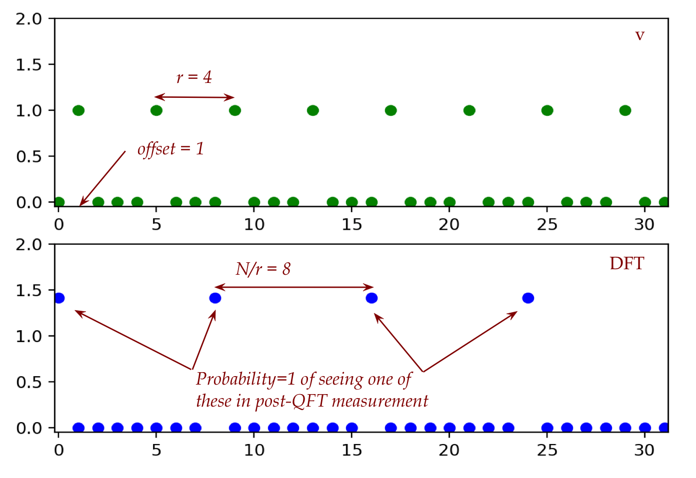
- First, consider a case where it does divide:
\(N=32, r=4, x_{f^\prime}=1\):
- Here, the offset is \(x_{f^\prime}=1\).
- We'll plot the classical DFT for the
vector
\(v=(0,1,0,0,0,1,0,0,0,1 \ldots, )\)
- And above, we'll plot \(v\) itself.
Here are both plots:

Note:
- The DFT perfectly captures the period \(r\) in its output.
- The DFT-output's period is not \(r\) but \(m = \frac{N}{r}\),
as shown earlier.
- Here, the output period is \(m = \frac{N}{r} = \frac{32}{4} = 8\).
- What does this imply for the QFT?
- The probability of seeing one of the \(\kt{y}\) states
where \(y = c\frac{N}{r}\) is \(1\).
- With different \(y_i = c_i\frac{N}{r}\) samples, one
can eventually infer \(\frac{N}{r}\).
This is what we saw in the previous section.
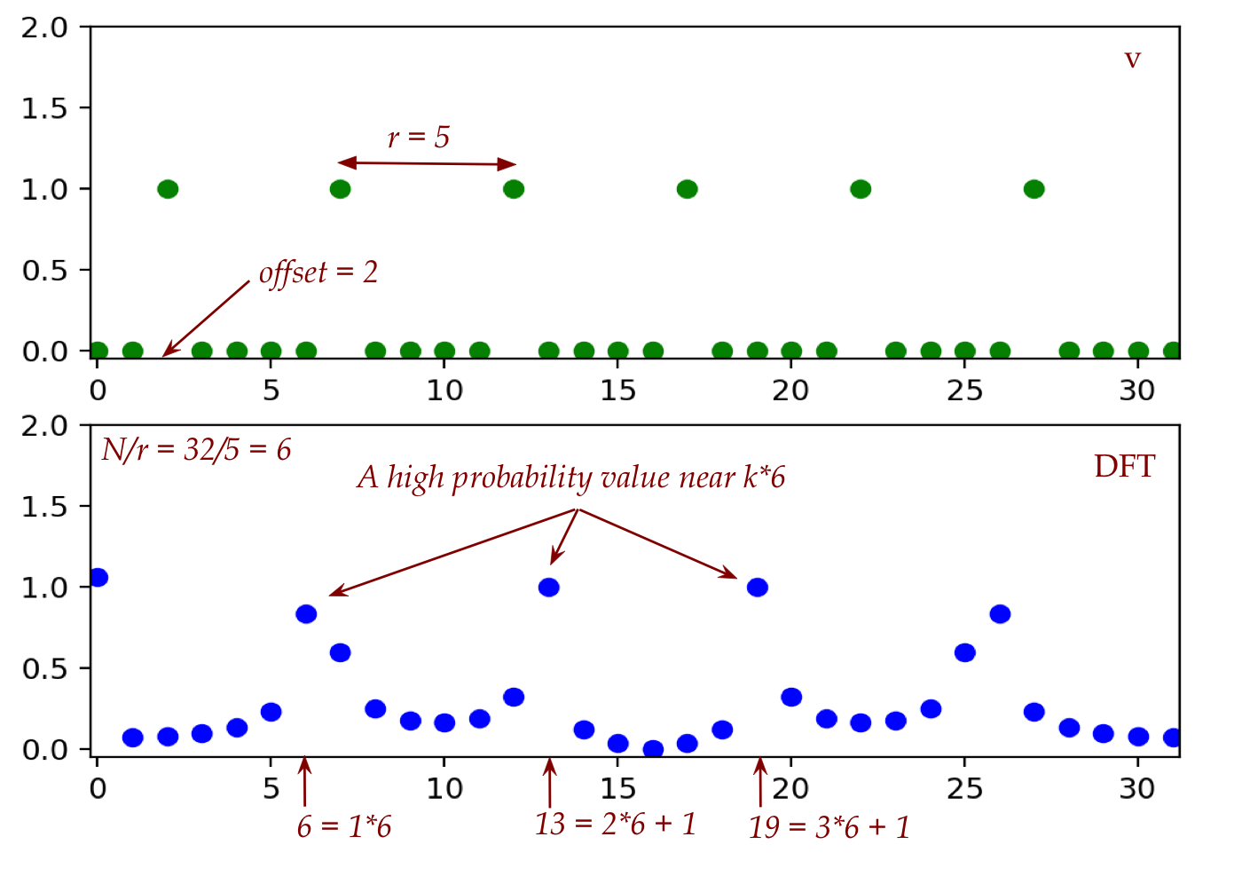
- Now let's examine a case where \(r\) does not divide \(N\):
- \(N=32, r=5\) with offset \(x_{f^\prime}=2\).
- In this case, \(m = \frac{N}{r} = \frac{32}{5} = 6\).
(Integer division.)
- Here are both plots:

Observe:
- The output is not as clean as we wished for.
- Nonetheless, there are DFT values
near multiples of \(m=6\).
- This might result in a high probability of seeing
one of these in the post-QFT measurement, provided
these high DFT-values have a high probability of being observed (measured).
To go further, we'll need to evaluate the probabilities
of obtaining states \(\kt{y}\) where \(y\) is near
a multiple \(c\frac{N}{r}\):
- To get "close enough" to an integer, all we need is to get
within \(\frac{1}{2}\) of the integer.
- Let \(\kt{y}\) be a state and let \(c\frac{N}{r}\)
be the nearest multiple of \(\frac{N}{r}\) near \(y\).
- Define
$$
\delta \eql y - c \frac{N}{r}
$$
And so
$$
y \eql c \frac{N}{r} + \delta
$$
- Recall the probability for any \(\kt{y}\):
$$
\magsq{\alpha_y}
\eql
\smf{1}{mN}
\magsq{ \sum_{k=0}^{m-1} w^{kry} }
$$
- We will now insert the expanded form of \(w\):
$$\eqb{
\magsq{\alpha_y}
& \eql &
\smf{1}{mN}
\magsq{ \sum_{k=0}^{m-1} e^{ \frac{2\pi i}{N} kry} }
& \mbx{With expansion of \(w\)} \\
& \eql &
\smf{1}{mN}
\magsq{ \sum_{k=0}^{m-1}
e^{ \frac{2\pi i}{N} kr(c \frac{N}{r} + \delta)} }
& \mbx{Sub for \(y\)} \\
& \eql &
\smf{1}{mN}
\magsq{ \sum_{k=0}^{m-1}
e^{ 2\pi i kc}
e^{ \frac{2\pi i}{N} kr\delta } }
& \mbx{Simplifying} \\
& \eql &
\smf{1}{mN}
\magsq{ \sum_{k=0}^{m-1}
e^{ \frac{2\pi i}{N} kr\delta } }
& \mbx{\(e^{ 2\pi i kc} = 1\)} \\
& \eql &
\smf{1}{mN}
\magsq{
\frac{ 1 - e^{ \frac{2\pi i}{N} r\delta m } }{ 1 - e^{
\frac{2\pi i}{N} r\delta} } }
& \mbx{Geometric sum} \\
}$$
- This looks hopelessly difficult, but let's press on.
In-Class Exercise 2:
Let \(z = 1 - e^{i\theta}\) and then use \(zz^*\) to show
that \(|z|^2 = 4 \sin^2 \frac{\theta}{2}\).
Continuing ...
- The exercise above shows that
$$
\magsq{1 - e^{i\theta}} \eql 4 \sin^2 \frac{\theta}{2}
$$
- Thus,
$$\eqb{
\magsq{\alpha_y}
& \eql &
\smf{1}{mN}
\magsq{
\frac{ 1 - e^{ \frac{2\pi i}{N} r\delta m } }{ 1 - e^{
\frac{2\pi i}{N} r\delta} } } \\
& \eql &
\smf{1}{mN}
\frac{
\sin^2 \parenl{ \frac{\pi r\delta m}{N} }
}{
\sin^2 \parenl{ \frac{\pi r\delta}{N} }
}
}$$
- Let's also recall what \(m\) is when \(r\) does not divide
\(N\):
- \(m\) is the number of \(x\)'s that have the particular
\(f^\prime\) from the first measurement.
- These are spaced apart with period \(r\).
- Because \(r\) does not divide \(N\), the integer \(m\)
is either
$$
m \eql \left\lfloor \frac{N}{r} \right\rfloor
$$
or
$$
m \eql \left\lfloor \frac{N}{r} \right\rfloor + 1
$$
- Thus, \(m \approx \frac{N}{r}\) for large \(N\) and \(r\).
- In the trigonometric numerator,
$$
\frac{\pi r\delta m}{N}
\eql
\frac{\pi \delta m}{N/r} \; \approx \; \pi\delta
$$
- In the corresponding denominator,
$$
\frac{\pi r\delta}{N}
\eql
\frac{\pi \delta}{N/r} \; \approx \; 0
$$
because, in RSA, \(N\) is large and one can expect
\(\frac{N}{r}\) to be large also.
- Then, one can use the approximation
\(\sin\theta \approx \theta\) for \(\theta \approx 0\).
- Substituting both of these:
$$\eqb{
\magsq{\alpha_y}
& \eql &
\smf{1}{mN}
\frac{
\sin^2 \parenl{ \frac{\pi r\delta m}{N} }
}{
\sin^2 \parenl{ \frac{\pi r\delta}{N} }
}\\
& \eql &
\smf{1}{mN}
\frac{
\sin^2 \parenl{ \pi\delta }
}{
\parenl{ \frac{\pi r\delta}{N} }^2
}\\
& \eql &
\smf{1}{mN} \frac{N^2}{r^2}
\frac{
\sin^2 \parenl{ \pi\delta }
}{
\pi^2 \delta^2
}\\
& \approx &
\frac{1}{r}
\left( \frac{\sin \pi\delta}{\pi\delta} \right)^2 \\
}$$
- Next, we'll need to dig a little deeper into the
behavor of \(\frac{\sin\theta}{\theta}\):
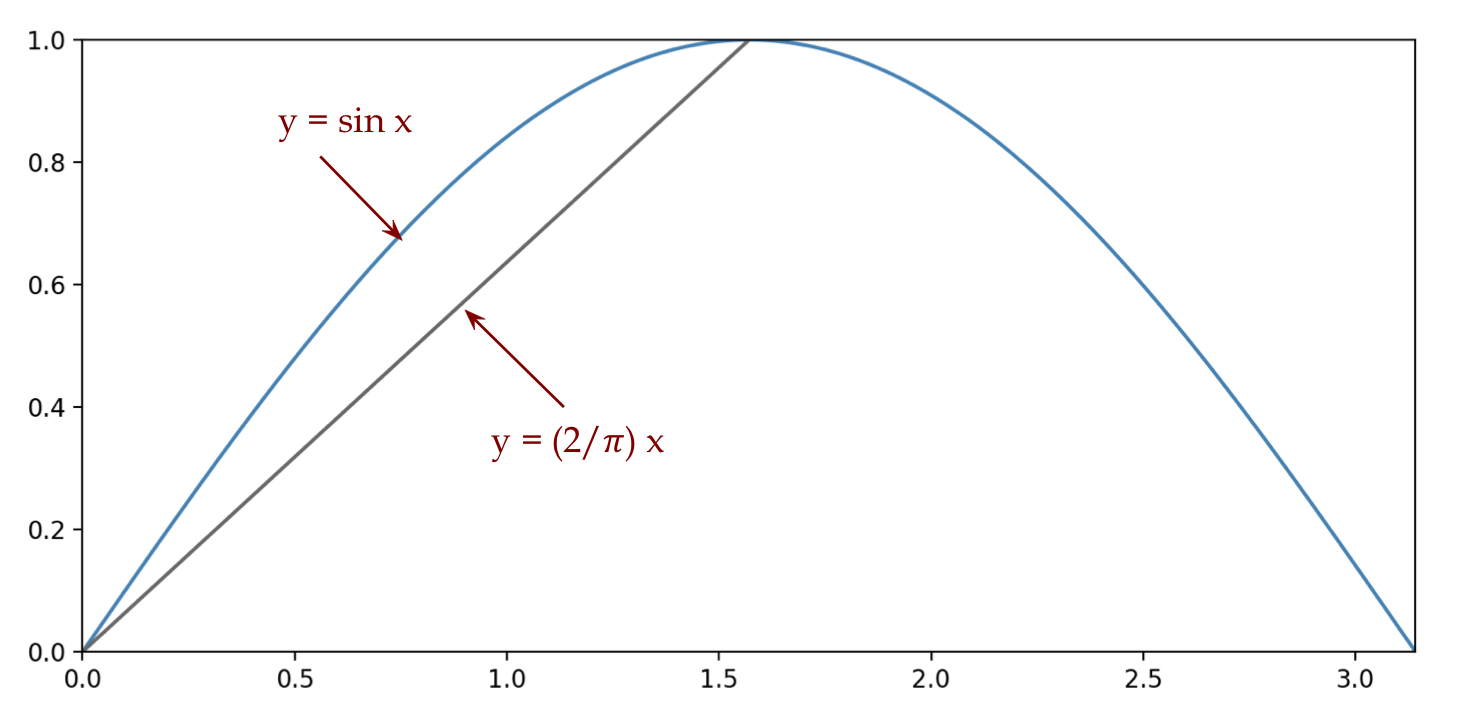
- Consider the graphs of \(y=\sin x\) and the line from
the origin to the top of the first crest:

- The graph of the line is
$$
y \eql \frac{2}{\pi} x
$$
- Clearly, in the range \(0 \leq x \eql \frac{\pi}{2}\),
$$
\sin x \; \geq \; \frac{2}{\pi} x
$$
- Now consider
$$
\frac{ \sin(\pi\delta) }{\pi\delta}
$$
- Recall that \(\delta \lt \frac{1}{2}\) because that is
the "error" bound we seek.
- Then
$$
\pi\delta \eql \pi \frac{1}{2}
$$
which places \(\pi\delta\) in the desired range.
- In this range,
$$
\frac{ \sin(\pi\delta) }{\pi\delta}
\geq
\frac{2\delta}{\pi\delta}
$$
- Thus, we can now substitute into the probability
$$\eqb{
\magsq{\alpha_y}
& \; \approx \; &
\frac{1}{r}
\left( \frac{\sin \pi\delta}{\pi\delta} \right)^2 \\
& \; \geq \; &
\frac{1}{r}
\frac{4}{\pi^2} \\
& \eql &
\frac{1}{r}
0.4
}$$
- This probability is a lower bound for a particular \(y\)
that's near a multiple of \(\frac{N}{r}\).
- There are \(r\) of these \(y\)'s:
- The gap from \(0\) to \(N\) has segments of length \(\frac{N}{r}\).
- Thus, there are \(\frac{N}{\frac{N}{r}} = r\) of them.
- Thus, finally, we see that
$$
\mbox{Pr[at least one of these \(y\)'s appear]}
\; \geq \;
\sum_{\mbox{all \(r\)}} \frac{1}{r} 0.4
\eql
0.4
$$
In other words, a 40% chance of getting an outcome that's with
\(\frac{1}{2}\) of \(c\frac{N}{r}\) for some \(c\).
10.9
A final step towards order-finding (that does work)
Let's recap where we are:
- We want to factor \(M\).
- That is, via order-finding: we want to find the order \(r\)
for some random \(a\) such that
$$
a^r \md M \eql 1
$$
and then work through the number theory involving
$$
(a^{\frac{r}{2}} + 1)(a^{\frac{r}{2}} - 1) \; \equiv_M \; 0
$$
- When we measure the \(f(x)\) qubits
after the order-computing \(U_f\), we get some
$$
\frac{1}{\sqrt{m}} \sum_{k=0}^{m-1} \kt{x_{f^\prime} + kr} \kt{f^\prime}
$$
- To get at the order \(r\) we apply the QFT and then measure
the top qubits, which removes \(x_{f^\prime}\) altogether.
- At this moment, we have found some \(\kt{y}\) such that
\(y\) is within \(\frac{1}{2}\) of \(c\frac{N}{r}\) for some \(c\):
- Here, \(r\) does not divide \(N\).
- And we don't know \(c\).
- Now for an important observation:
- The periodic behavior in the QFT's output will occur for
any \(N\) that's large enough.
- We can make \(N\) as large as we like.
- The very minimum is: \(N \gt M\).
Now let's focus on a useful choice of \(N\):
- By choosing \(N\), we mean choosing \(n\), the number of
qubits (because \(2^n = N\)).
- Suppose we pick \(N \gt M^2\):
- That is, enough qubits \(n\) so that \(2^n \gt M^2\).
- Now recall that we've found \(y\) (with high enough
probability) such that
$$
\mag{ y - c\frac{N}{r} } \leq \frac{1}{2}
$$
which means
$$
\mag{ \frac{y}{N} - \frac{c}{r} } \leq \frac{1}{2N} \lt \frac{1}{2M^2}
$$
- Now, one could imagine that there are many such rationals
\(\frac{c_1}{r_1}, \frac{c_2}{r_2}, \ldots\)
that are "close" enough to \(y\):
- Only one of these will have \(r_i=r\) that we seek.
- How do we find this particular rational?
To find \(r\), we exploit a number-theory result about
continued fractions:
- Recall
Proposition A.2.8
from the Appendix:
Proposition A.2.8:
Suppose \(x\) and \(\frac{a}{b}\) are rational numbers such that
$$
\mag{ x - \frac{a}{b} } \leq \frac{1}{2b^2}
$$
Then, \(\frac{a}{b}\) is a convergent in the continued-fraction
expansion of \(x\).
- Here, \(\frac{y}{N}\) is the rational that we have in hand:
the result of measuring after applying the QFT.
- And, we know the condition is satisfied, because we showed
that
$$
\mag{ \frac{y}{N} - \frac{c}{r} } \lt \frac{1}{2M^2}
$$
- This means the rational, and thus both integers
\(c\) and \(r\), will show up in the continued fraction
expansion of \(\frac{y}{N}\).
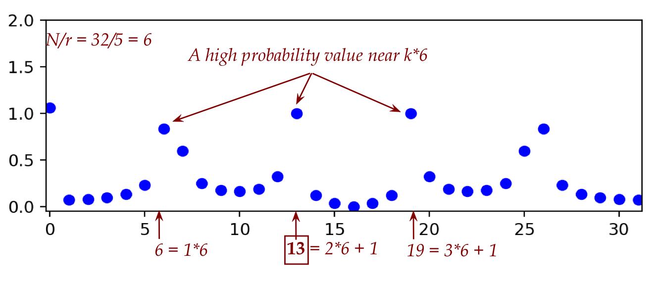
- For example, let's go back to our DFT output picture:

Suppose we happen to have \(y=13\) as the measured output.
- Thus,
$$
\frac{y}{N} = \frac{13}{32}
$$
in this example.
- We find the continued fraction expansion of \(\frac{13}{32}\)
$$
\frac{13}{32}
\eql
0 + \cfrac1{ 2 + \cfrac1{ 2 + \frac{1}{6}} }
$$
- The convergents for this are:
$$\eqb{
g_1 & \eql &
0 + \cfrac1{ 2 }
& \eql & \frac{1}{2} \\
g_2 & \eql &
0 + \cfrac1{ 2 + \cfrac1{ 2 }}
& \eql & \frac{2}{5} \\
g_3 & \eql &
0 + \cfrac1{ 2 + \cfrac1{ 2 + \frac{1}{6}} }
& \eql & \frac{13}{32} \\
}$$
- Thus, the possibilities for \(r\) are the three denominators
above: \(r\in \{2,5,32\}\).
- We could simply try all these potential \(r\) values.
- However, a further optimization can be achieved by examining
$$
\mag{ y - c\frac{N}{r} } \leq \frac{1}{2}
$$
- Compute \(y - N\frac{c}{r}\) for each potential convergent \(\frac{c}{r}\).
- For example:
$$
\mag{ y - N\frac{2}{r} }
\eql
\mag{ 13 - 32\frac{2}{5} }
\eql
\mag{ 13 - 12.8}
\lt \frac{1}{2}
$$
- This suggests that \(r=5\) is a good candidate.
- On the other hand,
$$
\mag{ 13 - 32\frac{1}{2} }
\eql
\mag{ 13 - 16}
\eql 4
\gt \frac{1}{2}
$$
So, \(r=2\) cannot work.
Finally, we have
an algorithm that works (with high probability): Shor's algorithm.
10.10
Summary: Shor's algorithm
Let's outline the steps
given \(M = pq\), the number to be factored:
Lastly, let's clarify the probabilistic part:
- Let's ask: what does it mean for an algorithm, where a
single run succeeds with probability \(\alpha\)?
- Then, the probability of failure is \(1-\alpha\).
- The probability of \(k\) repeated failures is
\( (1-\alpha)^k \).
- If \(\alpha\) is reasonably large, then \( (1-\alpha)^k \)
is going to be really small.
- For Shor's algorithm, there are several uncertainties:
- The probability of getting \(r\) out of the QFT: this is
at least \(0.4\).
- The probability of even \(r\) is: \(0.5\)
- The probability of \((a^{\frac{r}{2}}+1 \md M) \neq 0\)
is high.
- Even if the product of these is \(0.4 \times 0.5 \times 0.5
= 0.1\), the probability of \(10\) successive failures is:
$$
(1 - 0.9)^{10} \eql (10^{-1})^{10} \eql 10^{-10}
$$
All that's left now is the question:
can modular-exponentiation and the QFT be implemented
efficiently in a quantum circuit?
10.11
Implementation: QFT
Could the reversibility approach that converts classical
circuits into quantum versions provide an efficient implementation?
- The classical FFT algorithm runs in time \(O(N \log N)\).
- Recall: \(N \gt M^2\) where \(M\) is large.
- Since \(2^n = N\), we can write this as \(O(2^n n)\).
- A direct conversion via reversibility
uses one qubit per classical complex number (the input to DFT)
\(\rhd\)
The quantum version will take at best \(O(2^n n)\).
- This calls for a directly designed quantum version that
will use \(n\) qubits to represent \(2^n\) complex numbers.
- We will show that such a circuit can be designed to
require at most \(O(n^2)\) gates.
- This ensures that a single run of the quantum circuit
runs in (small) polynomial-time.
Let's begin with a few insights:
- The first insight: we only need to design the QFT to work on standard-basis
vectors:

- The inputs to Shor's algorithm are integers, whose
order we want to find via \(a^x \md M\).
- What goes into the QFT are the top (left) qubits in
$$
\smf{1}{\sqrt{m}} \sum_{k=0}^{m-1} \kt{x_{f^\prime} + kr} \kt{f^\prime}
$$
(each term is a standard-basis vector)
- Recall the action of \(U_{\smb{QFT}}\)
on any standard-basis \(\kt{x}\):
$$
U_{\smb{QFT}} \kt{x}
\eql
\smf{1}{\sqrt{N}} \sum_{y=0}^{N-1} w^{xy} \kt{y}
$$
where \(w=e^{ \frac{2\pi i}{N}}\), the principal \(N\)-th root of \(1\).
- Our goal now is: design a circuit for \(U_{\smb{QFT}}\).
- Now substitute the expanded form of \(w\)
into the expression above:
$$
U_{\smb{QFT}} \kt{x}
\eql
\smf{1}{\sqrt{N}} \sum_{y=0}^{N-1} e^{ \frac{2\pi i xy}{N}} \kt{y}
$$
Notice:
- For different \(y\), the product \(xy\) will change.
- Each such \(xy\) results in a different angle
\(\frac{2\pi xy}{N}\)
- These angles then determine the complex amplitudes in the
expression.
- And, what is the gate that changes angles? It's the \(P(\theta)\)
we saw earlier (Module 6):
$$
P(\theta) \eql
\mat{ 1 & 0 \\
0 & e^{i\theta} }
$$
- The second insight is that, because both \(\kt{x},\kt{y}\)
are standard-basis vectors, we can write them out in binary:
$$\eqb{
x & \eql & x_{n-1} x_{n-2} \ldots x_1 x_0
& \eql & 2^{n-1} x_{n-1} + 2^{n-1} x_{n-1} + \ldots +
2^{1} x_1 + x_0 \\
y & \eql & y_{n-1} y_{n-2} \ldots y_1 y_0
& \eql & 2^{n-1} y_{n-1} + 2^{n-1} y_{n-1} + \ldots +
2^{1} y_1 + y_0 \\
}$$
Also, the vectors \(\kt{x},\kt{y}\) can be written
in tensored form when convenient:
$$\eqb{
\kt{x} & \eql & \kt{x_{n-1}} \kt{x_{n-2}} \ldots \kt{x_1} \kt{x_0} \\
\kt{y} & \eql & \kt{y_{n-1}} \kt{y_{n-2}} \ldots \kt{y_1} \kt{y_0} \\
}$$
We will exploit both decompositions below.
- The third insight comes from the \(n=1\) (\(N=2\))
single qubit case:
- Let's write out the matrix:
$$
U_{\smb{QFT}}
\eql
\isqts{1}
\mat{ 1 & 1 \\
1 & w}
$$
- But, here,
$$
w \eql e^{ \frac{2\pi i}{N}} \eql e^{ \frac{2\pi i}{2}}
\eql e^{\pi i} \eql -1
$$
- Thus,
$$
U_{\smb{QFT}}
\eql
\isqts{1}
\mat{ 1 & 1 \\
1 & -1}
\eql H
$$
That is, the Hadamard gate.
- This sets up a goal: to use 1-qubit Hadamard gates
along with phase-changes with \(P(\theta)\) gates.
The controlled phase-shift gate:
- Recall the phase-shift gate \(P(\theta)\):
$$
P(\theta) \eql
\mat{ 1 & 0 \\
0 & e^{i\theta} }
$$
The action on 1-qubit standard-basis vectors is:
$$\eqb{
P(\theta) \kt{0}
& \eql &
\mat{ 1 & 0 \\
0 & e^{i\theta} } \mat{1 \\ 0}
& \eql & \kt{0} \\
P(\theta) \kt{1}
& \eql &
\mat{ 1 & 0 \\
0 & e^{i\theta} } \mat{0 \\ 1}
& \eql & e^{i\theta} \kt{1} \\
}$$
And on a generic vector:
$$
P(\theta) \parenl{\alpha \kt{0} + \beta \kt{1}}
\eql
\alpha \kt{0} + e^{i\theta} \beta \kt{1}
$$
which is where we see the relative change-of-phase.
- Suppose we wish to control whether or not such a
phase-change is applied in the 2-qubit case:
- When the top-qubit is \(\kt{0}\), no change.
- When the top-qubit is \(\kt{1}\), change the phase as above.
- Then, using Dirac notation, we'd write this as:
$$
Q(\theta) \eql \otr{0}{0} \otimes I \, + \, \otr{1}{1}
\otimes P(\theta)
\eql
\mat{1 & 0 & 0 & 0\\
0 & 1 & 0 & 0\\
0 & 0 & 1 & 0\\
0 & 0 & 0 & e^{i\theta}}\\
$$
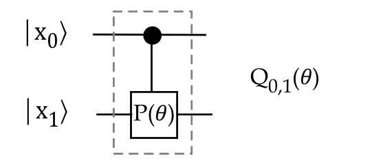
- Eventually, we're going to need to let qubit \(j\)
control the phase-shift for qubit \(k\):
- We'll use \(Q_{j,k}(\theta)\) as notation for this unitary.
- Then,
$$\eqb{
Q_{j,k}(\theta)
& \eql &
I_1 \otimes \ldots \otimes I_{j-1}
\otimes {\bf \otr{0}{0}_j}
\otimes I_{j+1} \otimes \ldots \otimes I_{k-1}
\otimes {\bf I_{k}}
\otimes I_{k+1} \otimes \ldots \otimes I_{n} \\
& \; &
\;\; + \;\;
I_1 \otimes \ldots \otimes I_{j-1}
\otimes {\bf \otr{1}{1}_j}
\otimes I_{j+1} \otimes \ldots \otimes I_{k-1}
\otimes {\bf P(\theta)}
\otimes I_{k+1} \otimes \ldots \otimes I_{n}
}$$
- For example, in a 5-qubit case where qubit 2 is the
control, and qubit 4 is the target:
$$\eqb{
Q_{2,4}(\theta)
& \eql &
I_1 \otimes {\bf \otr{0}{0}_2} \otimes I_3 \otimes {\bf I_4}
\otimes I_5 \\
& &
+ \; I_1 \otimes {\bf \otr{1}{1}_2} \otimes I_3 \otimes {\bf P(\theta)}
\otimes I_5 \\
}$$
Let's first work out the QFT circuit for the case \(n=2\):
- In this case \(w = e^{\frac{2\pi i}{N}} = e^{\frac{2\pi i}{4}}\)
- To avoid small fonts, we can also write
\(e^{\frac{2\pi i}{4}} = \exp(\frac{2\pi i}{4}) \)
- We will also make use of the binary forms
$$\eqb{
x & \eql & 2x_1 + x_0 \\
y & \eql & 2y_1 + y_0
}$$
Why binary forms?
- Gates act on qubits
- So, to build circuits, we need to track the states of individual
qubits
- Next,
$$\eqb{
U_{\smb{QFT}} \kt{x}
& \eql &
\smf{1}{\sqrt{4}}
\sum_{y=0}^3 w^{xy} \kt{y} \\
& \eql &
\smf{1}{2}
\sum_{y=0}^3 \exps{\frac{2\pi i}{4} xy} \kt{y} \\
& \eql &
\smf{1}{2}
\sum_{y_1,y_0\in\{0,1\}} \exps{\frac{2\pi i}{4} x(2y_1+y_0)} \kt{y_1}\kt{y_0} \\
& \eql &
\smf{1}{2}
\left(
\sum_{y_1\in\{0,1\}} \exps{\frac{2\pi i}{4} x(2y_1) } \, \kt{y_1}
\right)
\, \otimes \,
\left(
\sum_{y_0\in\{0,1\}} \exps{\frac{2\pi i}{4} x(y_0) } \, \kt{y_0}
\right) \\
& \eql &
\smf{1}{2}
\left(
\kt{0} \, + \, \exps{\frac{2\pi i}{4} 2x} \, \kt{1}
\right)
\, \otimes \,
\left(
\kt{0} \, + \, \exps{\frac{2\pi i}{4} x} \, \kt{1}
\right) \\
}$$
- Next, we'll expand \(x\) in binary:
$$\eqb{
U_{\smb{QFT}} \kt{x}
& \eql &
\smf{1}{2}
\left(
\kt{0} \, + \, \exps{\frac{2\pi i}{4} 2x} \, \kt{1}
\right)
\, \otimes \,
\left(
\kt{0} \, + \, \exps{\frac{2\pi i}{4} x} \, \kt{1}
\right) \\
& \eql &
\smf{1}{2}
\left(
\kt{0} \, + \, \exps{\frac{2\pi i}{4} 2(2x_1+x_0)} \, \kt{1}
\right)
\, \otimes \,
\left(
\kt{0} \, + \, \exps{\frac{2\pi i}{4} (2x_1+x_0)} \, \kt{1}
\right) \\
}$$
- Consider the first exponential:
$$\eqb{
\exps{\frac{2\pi i}{4} 2(2x_1+x_0)}
& \eql &
\exps{2\pi i x_1} \exps{\pi i x_0} \\
& \eql &
e^{2\pi i x_1} e^{\pi i x_0} \\
& \eql &
\parenl{ e^{2\pi i} }^{x_1} \parenl{e^{\pi i}}^{x_0} \\
& \eql &
1^{x_1} (-1)^{x_0} \\
& \eql &
(-1)^{x_0} \\
}$$
- The second one simplifies to:
$$\eqb{
\exps{\frac{2\pi i}{4} (2x_1+x_0)}
& \eql &
\exps{\pi i x_1} \exps{\frac{\pi}{2} i x_0} \\
& \eql &
e^{\pi i x_1} e^{\frac{\pi}{2} i x_0} \\
& \eql &
e^{\pi i x_1} e^{\frac{\pi}{2} i x_0} \\
& \eql &
(-1)^{x_1} e^{\frac{\pi}{2} i x_0} \\
}$$
- Substituting back,
$$\eqb{
U_{\smb{QFT}} \kt{x}
& \eql &
\smf{1}{2}
\left(
\kt{0} \, + \, \exps{\frac{2\pi i}{4} 2(2x_1+x_0)} \, \kt{1}
\right)
\, \otimes \,
\left(
\kt{0} \, + \, \exps{\frac{2\pi i}{4} (2x_1+x_0)} \, \kt{1}
\right) \\
& \eql &
\smf{1}{2}
\left(
\kt{0} \, + \, (-1)^{x_0} \kt{1}
\right)
\, \otimes \,
\left(
\kt{0} \, + \, (-1)^{x_1} e^{\frac{\pi}{2} i x_0} \kt{1}
\right) \\
}$$
In here, we see a Hadamard on the left, and a Hadamard-with-phase
on the right.
- The actual phase applies on the right only when \(x_0=1\):
- This suggests using \(x_0\) as the control bit to decide
whether or not to apply the phase change.
- The phase change is itself \(\frac{\pi}{2}\)
- We earlier introduced the notation
$$
Q_{0,1}(\theta) \eql
\mbox{ qubit 0 controls applying phase=\(\theta\) to qubit 1}
$$
- For the moment we'll assume top-to-bottom numbering starting
with \(0\):

- With this controlled-phase gate, we can now write
$$\eqb{
U_{\smb{QFT}} \kt{x}
& \eql &
\smf{1}{2}
\left(
\kt{0} \, + \, (-1)^{x_0} \kt{1}
\right)
\, \otimes \,
\left(
\kt{0} \, + \, (-1)^{x_1} e^{\frac{\pi}{2} i x_0} \kt{1}
\right) \\
& \eql &
\smf{1}{2}
\left(
\kt{0} \, + \, (-1)^{x_0} \kt{1}
\right)
\, \otimes \,
Q_{0,1}(\sml{\frac{\pi}{2}})
\left(
\kt{0} \, + \, (-1)^{x_1} \kt{1}
\right) \\
& \eql &
\parenl{(H \otimes I)
\,
Q_{0,1}(\sml{\frac{\pi}{2}}) \,
(I \otimes H) } \kt{x_0}\kt{x_1}
}$$
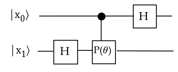
- We can draw the right side as:

Note:
- The Hadamard is applied to the first qubit after its
control value is used for the second.
- The 2nd qubit Hadamard is applied before the
phase-shift, because the phase-shift is applied to the Hadamard
superposition.
- There is one more piece of the puzzle:
- Recall how we write the binary form \(U_{\smb{QFT}} \kt{x}\):
$$
U_{\smb{QFT}} \kt{x} \eql U_{\smb{QFT}} \kt{x_1}\kt{x_0}
$$
- That is, the more significant bits are to the left.
- Yet, as the diagram shows, we want to apply
$$
\parenl{(H \otimes I)
\,
Q_{0,1}(\sml{\frac{\pi}{2}}) \,
(I \otimes H) } \kt{x_0}\kt{x_1}
$$
where the bits appear in reverse order.
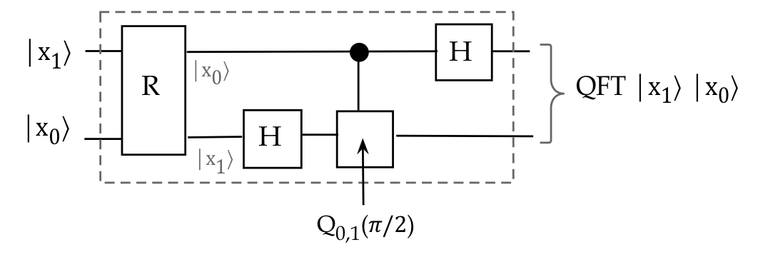
- Accordingly, we'll devise a gate \(R\) to reverse bit order
before feeding the qubits into the Hadamards and phase-change:
$$\eqb{
U_{\smb{QFT}} \kt{x}
& \eql & U_{\smb{QFT}} \kt{x_1}\kt{x_0}\\
& \eql &
\parenl{(H \otimes I)
\,
Q_{0,1}(\sml{\frac{\pi}{2}}) \,
(I \otimes H) } R \kt{x_1}\kt{x_0}\\
}$$
- We can now draw this as:

Before we get to higher values of \(n\), a useful result:
- Recall that
$$
U_{\smb{QFT}} \kt{x}
\eql
\smf{1}{\sqrt{N}} \sum_{y=0}^{N-1} e^{ \frac{2\pi i xy}{N} \kt{y}}
$$
- We will at different times substitute
$$\eqb{
x & \eql & \sum_{j=0}^{n-1} x_j 2^j \\
y & \eql & \sum_{j=0}^{n-1} y_j 2^j \\
}$$
- Substituting for \(y\):
$$\eqb{
U_{\smb{QFT}} \kt{x}
& \eql &
\smf{1}{\sqrt{N}} \sum_{y=0}^{N-1} e^{ \frac{2\pi i xy}{N} } \kt{y}\\
& \eql &
\smf{1}{\sqrt{N}} \sum_{y=0}^{N-1}
\exps{ \frac{2\pi i}{N} x \sum_{j} y_j2^j } \,
\kt{y} \\
& \eql &
\smf{1}{\sqrt{N}}
\sum_{y_{n-1},\ldots,y_0\in\{0,1\}}
\left(
\exps{ \frac{2\pi i}{N} x y_{n-1}2^{n-1} } \ldots
\exps{ \frac{2\pi i}{N} x y_0 2^0 }
\right) \,
\parenl{ \kt{y_{n-1}} \otimes \ldots \otimes \kt{y_0} }\\
& \eql &
\smf{1}{\sqrt{N}}
\sum_{y_{n-1},\ldots,y_0\in\{0,1\}}
\exps{ \frac{2\pi i}{N} x y_{n-1}2^{n-1} } \kt{y_{n-1}}
\otimes \ldots \otimes
\exps{ \frac{2\pi i}{N} x y_0 2^0 } \kt{y_0} \\
& \eql &
\smf{1}{\sqrt{N}}
\left(
\sum_{y_{n-1}\in\{0,1\}}
\exps{ \frac{2\pi i}{N} x y_{n-1}2^{n-1} } \kt{y_{n-1}}
\right)
\; \otimes \; \ldots \; \otimes \;
\left(
\sum_{y_{0}\in\{0,1\}}
\exps{ \frac{2\pi i}{N} x y_{0}2^{0} } \kt{y_{0}}
\right) \\
& \eql &
\smf{1}{\sqrt{N}}
\left(
\kt{0} \, + \,
\exps{ \frac{2\pi i}{2^n} x 2^{n-1} } \kt{1}
\right)
\; \otimes \; \ldots \; \otimes \;
\left(
\kt{0} \, + \,
\exps{ \frac{2\pi i}{2^n} x 2^{0} } \kt{1}
\right)
}$$
where we now only have terms with \(x\) and powers of \(2\).
- Next, consider the k-th term:
$$\eqb{
\exps{ \frac{2\pi i}{2^n} x2^k}
& \eql &
\exps{ \frac{2\pi i}{2^n} 2^k \sum_j x_j 2^j }\\
& \eql &
\exps{ 2\pi i (
\frac{x_0}{2^{n-k}} + \frac{x_1}{2^{n-k-1}}
+ \ldots + \frac{x_{n-1}}{2^{n-k-(n-1)}} ) } \\
& \eql &
\exps{ 2\pi i \frac{x_0}{2^{n-k}} }
\exps{ 2\pi i \frac{x_1}{2^{n-k-1}} }
\ldots
\exps{2\pi i \frac{x_{n-1}}{2^{n-k-(n-1)}} }
}$$
- Examine the last term to see that
$$\eqb{
\exps{ 2\pi i \frac{x_{n-1}}{2^{n-k-(n-1)}} }
& \eql & \exps{ 2\pi i \frac{x_{n-1}}{2^{1-k}} }\\
& \eql & \exps {2\pi i x_{n-1} 2^{k-1} } \\
& \eql & \parenl{ \exps {2\pi i x_{n-1} }^{2^{k-1} }} \\
& \eql & \parenl{ 1 }^{2^{k-1}} \\
& \eql & 1
}$$
- Thus, when the denominator in
$$
\exps{ 2\pi i \frac{x_{n-1}}{2^{n-k-j}} }
$$
is negative for the j-th term, that term will result in a power of \(1\).
- This happens for \(j \geq n-k\).
- Hence,
$$\eqb{
& \; &
\exps{ 2\pi i \frac{x_0}{2^{n-k}} }
\exps{ 2\pi i \frac{x_1}{2^{n-k-1}} }
\ldots
\exps{2\pi i \frac{x_{n-1}}{2^{n-k-(n-1)}} } \\
& \eql &
\exps{ 2\pi i \frac{x_0}{2^{n-k}} }
\exps{ 2\pi i \frac{x_1}{2^{n-k-1}} }
\ldots
\exps{2\pi i \frac{x_{n-1}}{2^{n-k-j}} }
}$$
- Now back to the \(U_{\smb{QFT}}\) from earlier:
$$
U_{\smb{QFT}} \kt{x} \eql
\smf{1}{\sqrt{N}}
\left(
\kt{0} \, + \,
\exps{ \frac{2\pi i}{2^n} x 2^{n-1} } \kt{1}
\right) \; \otimes \; \ldots \; \otimes \;
\left(
\kt{0} \, + \,
\exps{ \frac{2\pi i}{2^n} x 2^{0} } \kt{1}
\right)
$$
- In the first term, \(k=n-1\) and so all the terms
after \(j \geq n-1\) vanish:
$$
\exps{ 2\pi i \frac{x_0}{2^{n-k}} }
\exps{ 2\pi i \frac{x_1}{2^{n-k-1}} }
\ldots
\exps{2\pi i \frac{x_{n-1}}{2^{n-k-j}} }
\eql
\exps{ 2\pi i \frac{x_0}{2} }
$$
- For the second tensor term, \(k=n-2\), and terms after
\(j \geq n-2\) vanish:
$$
\exps{ 2\pi i \frac{x_0}{2^{n-k}} }
\exps{ 2\pi i \frac{x_1}{2^{n-k-1}} }
\ldots
\exps{2\pi i \frac{x_{n-1}}{2^{n-k-j}} }
\eql
\exps{ 2\pi i \frac{x_0}{2^{2}} }
\exps{ 2\pi i \frac{x_1}{2^1} }
$$
- And the third term in the tensor will be
$$
\exps{ 2\pi i \frac{x_0}{2^{3}} }
\exps{ 2\pi i \frac{x_1}{2^{2}} }
\exps{ 2\pi i \frac{x_2}{2^{1}} }
$$
- We will apply this in the \(n=3\) case next.
We'll now generalize by working through the \(n=3\) case:
- We showed above that for \(n=3\),
$$\eqb{
& \; &
U_{\smb{QFT}} \kt{x_2, x_1, x_0} \\
& \eql &
\smf{1}{\sqrt{2^3}}
\left(
\kt{0} \, + \,
\exps{ 2\pi i \frac{x_0}{2} } \kt{1}
\right)
\; \otimes \;
\left(
\kt{0} \, + \,
\exps{ 2\pi i (\frac{x_1}{2} + \frac{x_0}{2^2}) } \kt{1}
\right)
\; \otimes \;
\left(
\kt{0} \, + \,
\exps{ 2\pi i (\frac{x_2}{2} + \frac{x_1}{2^2} + \frac{x_0}{2^3}) } \kt{1}
\right)
}$$
- Let's examine the three terms above one by one.
- The first term is just:
$$\eqb{
& \; &
\kt{0} \, + \,
\exps{ 2\pi i \frac{x_0}{2} } \kt{1} \\
& \eql &
\kt{0} \, + \,
\exps{ \pi i x_0 } \kt{1} \\
& \eql &
\kt{0} \, + \,
(-1)^{x_0} \kt{1} \\
& \eql &
H \kt{x_0} \\
}$$
This is a Hadamard on the \(x_0\) qubit.
- The second term:
$$\eqb{
& \; &
\kt{0} \, + \,
\exps{ 2\pi i (\frac{x_1}{2} + \frac{x_0}{2^2}) } \kt{1} \\
& \eql &
\kt{0} \, + \,
\exps{ \pi i x_1 } \exps{ 2\pi i \frac{x_0}{2^2}) } \kt{1} \\
& \eql &
\kt{0} \, + \,
(-1)^{x_1} \exps{ 2\pi i \frac{x_0}{2^2}) } \kt{1} \\
& \eql &
Q_{0,1}(\sml{\frac{\pi}{2}})
\parenl{ \kt{0} \, + \, (-1)^{x_1} \kt{1} } \\
}$$
That is, the phase of \(\frac{\pi}{2}\) is applied only if
\(x_0=1\), i.e., controlled by \(x_0\).
- The third term:
$$\eqb{
& \; &
\kt{0} \, + \,
\exps{ 2\pi i (\frac{x_2}{2} + \frac{x_1}{2^2} +
\frac{x_0}{2^3}) } \kt{1} \\
& \eql &
\kt{0} \, + \,
(-1)^{x_2} \exps{2\pi i \frac{x_1}{2^2}} \exps{2\pi
i\frac{x_0}{2^3}} \kt{1} \\
& \eql &
Q_{0,2}(\sml{\frac{\pi}{4}})
Q_{1,2}(\sml{\frac{\pi}{2}})
\parenl{ \kt{0} \, + \, (-1)^{x_2} \kt{1} } \\
}$$
Thus, there are now two phases that apply to the \(x_2\)
qubit, controlled by \(x_0\) and \(x_1\),
each with a different angle.
- Thus, we've shown
$$\eqb{
& \; &
U_{\smb{QFT}} \kt{x_2, x_1, x_0} \\
& \eql &
\parenl{H \otimes I \otimes I}
\parenl{Q_{0,1}(\sml{\frac{\pi}{2}})}
\parenl{I \otimes H \otimes I}
\parenl{
Q_{0,2}(\sml{\frac{\pi}{4}})
Q_{1,2}(\sml{\frac{\pi}{2}})
}
\parenl{I \otimes I \otimes H}
\,
\kt{x_0, x_1, x_2}
}$$
- Once again, since the order needed by the operators is
the opposite, we'll use a 3-qubit "reverse" operator \(R\):
$$\eqb{
& \; &
U_{\smb{QFT}} \kt{x_2, x_1, x_0} \\
& \eql &
\parenl{H \otimes I \otimes I}
\parenl{Q_{0,1}(\sml{\frac{\pi}{2}})}
\parenl{I \otimes H \otimes I}
\parenl{
Q_{0,2}(\sml{\frac{\pi}{4}})
Q_{1,2}(\sml{\frac{\pi}{2}})
}
\parenl{I \otimes I \otimes H}
\,
R \, \kt{x_2, x_1, x_0}
}$$
- Finally, let's draw the circuit:

Note:
- A Hadamard is applied to each qubit.
- However, before that Hadamard is applied, the qubit
applies itself as control to all needed controls.
- For example, the top qubit above is used as control
twice before being subject to \(H\).
Generalization to \(n\) qubits:
- The same idea above extends to \(n\) qubits.
- The qubits start in \(\kt{x_{n-1}}\kt{x_{n-2}}\ldots \kt{x_0}\).
- They are reversed to
\(\kt{x_{0}} \ldots \kt{x_{n-2}}\kt{x_{n-1}}\).
- Each qubit line \(k\) has a Hadamard first applied,
and then one \(Q_{j,k}(\theta_{j,k})\) controlled by
each qubit \(j\) above.
- The angle dependence depends the difference \(k-j\):
$$
\theta_{j,k} \eql \frac{\pi}{2^{k-j}}
$$
Finally, let's count the gates:
- The reversing of \(n\) qubits requires \(n\) 2-qubit swaps.
- Each qubit line of the QFT has \(n\) Hadamards.
- The last qubit has \(n-1\) controlled phase-shifts,
the qubit \(n-2\) has \(n-2\) phase-shifts, and so on.
- This adds up to \((n-1) + (n-2) + \ldots + 1 = \frac{n(n-1)}{2}\)
Q gates.
- Thus, overall: \(2n + \frac{n(n-1)}{2} = O(n^2)\) gates.
Whew!
10.12
A QFT result that's useful in other algorithms
One way to write the different terms in the output of the QFT
turns out to be useful in other algorithms:
- Let's start with the basic QFT expression derived earlier
when applied to a standard-basis vector \(\kt{x}\):
$$
U_{\smb{QFT}} \kt{x} \eql
\smf{1}{\sqrt{N}}
\left(
\kt{0} \, + \,
\exps{ \frac{2\pi i}{2^n} x 2^{n-1} } \kt{1}
\right)
\; \otimes \; \ldots \; \otimes \;
\left(
\kt{0} \, + \,
\exps{ \frac{2\pi i}{2^n} x 2^{0} } \kt{1}
\right)
$$
- Here, the coefficient of \(\kt{1}\) in the k-th term is
$$\eqb{
\exps{ \frac{2\pi i}{2^n} x2^k}
& \eql &
\exps{ \frac{2\pi i}{2^n} 2^k \sum_j x_j 2^j }\\
& \eql &
\exps{ 2\pi i (
\frac{x_0}{2^{n-k}} + \frac{x_1}{2^{n-k-1}}
+ \ldots + \frac{x_{n-1}}{2^{n-k-(n-1)}} ) } \\
& \eql &
\exps{ 2\pi i \frac{x_0}{2^{n-k}} }
\exps{ 2\pi i \frac{x_1}{2^{n-k-1}} }
\ldots
\exps{2\pi i \frac{x_{n-1}}{2^{n-k-(n-1)}} }
}$$
- We showed that this simplifies as the following pattern:
- When \(k=n-1\) (the leftmost term) we get
$$
\exps{ 2\pi i \frac{x_0}{2} }
$$
which we'll write as
$$
\exps{ 2\pi i (0.x_0) }
$$
- With \(k=n-2\), we get
$$
\exps{ 2\pi i \frac{x_0}{2^{2}} }
\exps{ 2\pi i \frac{x_1}{2^1} }
\eql
\exps{ 2\pi i (0.x_1 x_0) }
$$
- With \(k=n-3\):
$$
\exps{ 2\pi i \frac{x_0}{2^{3}} }
\exps{ 2\pi i \frac{x_1}{2^{2}} }
\exps{ 2\pi i \frac{x_2}{2^{1}} }
\eql
\exps{ 2\pi i (0.x_2 x_1 x_0) }
$$
- And so on.
- Now, the \(x_i\)'s are the binary digits of \(x\), so we
can write
$$\eqb{
\kt{x} & \eql & \kt{x_{n-1} \ldots x_1 x_0} \\
& \eql & \kt{x_{n-1}} \ldots \kt{x_1} \kt{x_0}
}$$
- Thus, one can write the QFT output as:
$$\eqb{
U_{\smb{QFT}} \kt{x}
& \eql &
U_{\smb{QFT}} \kt{x_{n-1}} \ldots \kt{x_1} \kt{x_0} \\
& \eql &
\smf{1}{\sqrt{N}}
\left(
\kt{0} \, + \,
\exps{ 2\pi i (0.x_0) } \kt{1}
\right) \\
& &
\; \otimes \;
\left(
\kt{0} \, + \,
\exps{ 2\pi i (0.x_1 x_0) } \kt{1}
\right) \\
& &
\; \otimes \;
\left(
\kt{0} \, + \,
\exps{ 2\pi i (0.x_2 x_1 x_0) } \kt{1}
\right) \\
& & \vdots \\
& &
\; \otimes \;
\left(
\kt{0} \, + \,
\exps{ 2\pi i (0.x_{n-1} \ldots x_0) } \kt{1}
\right)
}$$
- Note:
- The binary digits of standard basis vector \(\kt{x}\)
appear in the coefficients on the right.
- If we somehow had access to binary digits of \(\kt{x}\)
and were able to successively turn them into coefficients like
those above, we could recover \(x\) using
the inverse:
$$\eqb{
\kt{x_{n-1} \ldots x_1 x_0} & \eql &
U_{\smb{QFT}}^{-1}
\smf{1}{\sqrt{N}}
\left(
\kt{0} \, + \,
\exps{ 2\pi i (0.x_0) } \kt{1}
\right) \\
& &
\; \otimes \;
\left(
\kt{0} \, + \,
\exps{ 2\pi i (0.x_1 x_0) } \kt{1}
\right) \\
& &
\; \otimes \;
\left(
\kt{0} \, + \,
\exps{ 2\pi i (0.x_2 x_1 x_0) } \kt{1}
\right) \\
& & \vdots \\
& &
\; \otimes \;
\left(
\kt{0} \, + \,
\exps{ 2\pi i (0.x_{n-1} \ldots x_0) } \kt{1}
\right)
}$$
This idea is used in finding eigenvalues, one of the more practical
applications of quantum computing.
