Note: some parts of the review (such as calculus) aren't needed
for quantum computing, but are presented as prelude to following
one's curiosity about quantum mechanics.
M.1 Sets and numbers
About sets:
- A set is a collection of 'things', most often numbers,
all of which have some reason to be considered as part of the
collection:
- Thus, while \(S = \{-4, 7, 19\}\) is indeed a set, one might
ask why the set \(S\) was defined as such.
- It's more common to have some meaning, such as
\(S = \{1^2, 2^2, \ldots, 10^2\}\), the set of squared
integers between 1 and 100 (inclusive).
- Sets can be small such as
- \(\{1, 2, 3\}\)
- \(\{\; \} \;\;\;\) (empty set, often denoted by \(\emptyset\))
or large such as
- \(\mathbb{N} = \{1, 2, 3, \ldots\}\), the set of natural numbers.
- \(\mathbb{Z} = \{\ldots, -3, -2, -1, 0, 1, 2, 3, \ldots\}\), the set of integers.
- \(\mathbb{Q} = \{\frac{p}{q}: \mbox{p and q are integers}\}\), the set of rational numbers.
- Sets are often depicted via a property that must be
satisfied to belong to the set, for example:
$$
\{{\bf x}: {\bf A x} = {\bf b}\}
\eql \mbox{ the set vectors that are solutions to the
matrix-vector equation } {\bf A x} = {\bf b}
$$
- What do we do with sets?
- We can apply operators (such as \( \cup, \cap, \prime\) )
that build sets out of other sets, for example:
$$
\{1,2,3\} \cup \{2, 3, 5\} \eql \{1, 2, 3, 5\}
\;\;\;\;\mbox{ union operator}
$$
- We can assess the size, for example, if
\(S = \{1,2,3,5\}\) then the cardinality
of \(|S| = 4\).
- Most often, however, sets are used to precisely pinpoint something
of mathematical interest, which we perhaps want to reason about, for
example:
$$
\mbox{span}({\bf u}, {\bf v})
\eql
\{ \alpha {\bf u} + \beta {\bf v}\}
$$
This is the set of all possible linear combinations of the vectors
\({\bf u}\) and \({\bf v}\), which we can write more
conventionally as:
$$
\mbox{span}({\bf u}, {\bf v})
\eql
\{ {\bf w}: {\bf w}= \alpha {\bf u} + \beta {\bf v}, \;
\alpha,\beta\in\mathbb{R}\}
$$
Sets of numbers:
- We're not going to go deep into numbers or number theory;
we'll only outline a few important sets by way of background.
- Natural numbers: \(\mathbb{N} = \{1, 2, 3, \ldots\}\)
- A set by itself has limited value until we 'do' something
with its elements.
- Thus we define the common and intuitive operators
\(+, -, \times, \div\).
- In doing so, we run into our first difficulty:
clearly \(5 - 2\) is in the set \(\mathbb{N}\) but
what about \(2 - 5\)?
- The difficulty is resolved by expanding our notion of
number.
- Integers:
\(\mathbb{Z} = \{\ldots, -3, -2, -1, 0, 1, 2, 3, \ldots\}\), the
set of integers.
- Now all additions, subtractions and multiplications give us
members of the same set.
- But division requires an expanded set of numbers.
- Rational numbers:
\(\mathbb{Q} = \{\frac{p}{q}: \mbox{p and q are integers}\}\)
- Now all four basic operators applied to any two members
of \(\mathbb{Q}\) results in a member of \(\mathbb{Q}\).
- Yet, there are other operations we seek to perform,
and soon discover that, for example,
\(\sqrt{2}\) is not rational.
- Real numbers:
- Real numbers are
actually tricky
to define rigorously.
- One can't simply add all square roots to the rationals: what
about the number that describes the ratio of a circle's
circumference to its diameter?
- We'll stick to an intuitive notion: the reals
\(\mathbb{R}\) are all the numbers we get from
common operations such as: arithmetic, powers, roots, limits.
- Once again, we run into a difficulty:
- We know that the equation \(x^2 = 2\) has a real number
solution.
- But \(x^2 = -2\) does not.
- Which finally leads to complex numbers, commonly denoted
by \(\mathbb{C}\):
- By introducing a symbol \(i\) to represent \(\sqrt{-1}\),
\((\sqrt{2}i)^2 = -2\).
- One representation of a complex number: \(a + bi\).
- Another (the polar representation): \(r e^{i\theta}\).
- And to a natural question: do we need anything beyond
complex numbers?
(We'll address this below.)
Let's point out a few highlights regarding sets of numbers:
- It is possible to reason about the cardinality (size) of
infinite sets.
- From which:
- \(\mathbb{N}, \mathbb{Z}, \mathbb{Q}\) all have the same
cardinality, commonly called countable.
- The cardinality of the reals (and complex numbers)
is larger, called uncountable.
- There are other oddities when reasoning about the different
sizes of infinity, for example: the number of points on the
plane has the same cardinality as the number of points on the line.
- Types of real numbers:
- Consider a polynomial like:
\(p(x) = -3 + x^2 + 3x^5\).
- It has long been of interest to solve equations like
\(p(x) = 0\) or to reason whether solutions can in fact be found.
- A algebraic real number \(\alpha\) is a number for which at
least one polynomial \(p(x)\) exists such that \(p(\alpha) = 0\).
- Thus, every algebraic number is the solution to some
polynomial equation, of which there are only a countable number.
- Therefore, the other reals (which are uncountable) can't be
solutions to a polynomial equation: we call
these transendental numbers.
- Examples are: \(\pi, e\).
- Polynomial equations may not have a real solution.
If, however, we include complex numbers as possible
solutions to polynomial equations, then every such equation has at
least one solution.
- This is known as the Fundamental Theorem of Algebra.
- The theorem says more: a degree-n polynomial has exactly
n complex roots (allowing for multiplicity).
Let's now turn to a few questions:
- Since the reals include the integers, why bother with integers?
- Recall the difficulty: division.
- We can in fact modify the division operator to give us
two operators that result in integers:
- The integer div operator, as in \(7 \mbox{ div } 3 = 2\)
- The integer remainder operator, as in \(7 \mbox{ mod } 3 = 1\)
- Of these, the remainder operator turns out to be the
interesting one, leading to modern applications like cryptography.
- Since complex numbers include the reals, why bother with reals?
- Reals are a bit easier to understand.
- And our real world has measurable quantities (length,
temperature, time) for which
real numbers are well-suited.
- Thus, even if we work with complex numbers, we'll want to
know how to extract a real part that's relevant to an application.
- Do we need anything beyond complex numbers?
- Surprisingly, the answer for us is: yes.
- We'll see that when we need to explain quantum phenomena,
what's needed is a bigger structure: a complex vector.
- One way to think of a complex number \(a + bi\) is that
it is a pair of real numbers \((a,b)\).
- Then, a 2-component complex vector
\((a+bi, c+di)\) can be considered a quadruple
of real numbers. This is what will be needed, as we'll see,
to represent a qubit.
M.2 Functions
What is a function?
- Intuitively, a function is something that "computes" a result
(another number) given an input.
- For example, \(f(x) = x^2\) takes a number \(x\) and
produces its square.
- Alternatively, we can think of a function as an association:
the square function associates every number with its
square, e.g.,
$$
\begin{array}{lll}
2
\;\;\;\;\; & \;\;\;\;\;
\mbox{is associated with}
\;\;\;\;\; & \;\;\;\;\;
4\\
3
\;\;\;\;\; & \;\;\;\;\;
\mbox{is associated with}
\;\;\;\;\; & \;\;\;\;\;
9\\
3.126
\;\;\;\;\; & \;\;\;\;\;
\mbox{is associated with}
\;\;\;\;\; & \;\;\;\;\;
9.771876\\
\end{array}
$$
Here, there is no specified computation.
The "association" view becomes useful when we
consider coordinates:
More about functions:
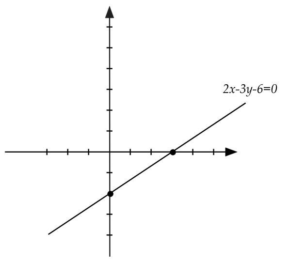
- We use the term locus to describe a set of
points satisfying a certain property.
- Example: consider all points \((x,y)\) such that
\(2x - 3y - 6 = 0\)
- We write this as \(\{(x,y): 2x-3y-6=0\}\).
- Or as a function: \(f(x) = (2x - 6) / 3 \)
- This turns out, geometrically, to be a line.
- Functions became much more useful and powerful when
associated with coordinate geometry:
- One could now algebraically describe the curves
that had already been well-studied:
$$\eqb{
\frac{x^2}{r^2} + \frac{y^2}{r^2} = 1
& \;\;\;\;\;\; &
\mbox{circle} \\
\frac{x^2}{a^2} + \frac{y^2}{b^2} = 1
& \;\;\;\;\;\; &
\mbox{ellipse} \\
\frac{x^2}{a^2} - \frac{y^2}{b^2} = 1
& \;\;\;\;\;\; &
\mbox{hyperbola} \\
y^2 - 4ax = 0
& \;\;\;\;\;\; &
\mbox{parabola} \\
}$$
And, moreover, exploit algebraic results to rigorously
derive new properties in full generality.
- There soon followed even more algebraic descriptions,
such as the parametric representation:
\(x(t) = r\cos(t), y(t)=r\sin(t)\) (circle).
- The general idea of and notation for single-variable
functions is easily extended to:
- Multiple variables, e.g. \(f(x,y,z)\)
- Function composition, e.g., \(f(g(x))\)
- An inverse of a function, \(f^{-1}(x)\)
Special classes of functions:
- With the development of the mathematics of functions, some
particular functions grew in significance.
- For example, polynomials occur in many contexts, and
are easy to understand, easy to calculate by hand.
- An important question then arose: are polynomials
good enough? That is, can any function be well-approximated by
some polynomial?
- The Stone-Weierstrass theorem confirmed the existence
of a polynomial \(p(x)\) such that \(|p(x) - f(x)| \lt
\epsilon\) when given \(f(x)\) and \(\epsilon\)
in the interval of interest.
- Bernstein showed that a linear combination of
(the later to be named) Bernstein polynomials could
arbitrarily closely approximate any continuous function.
- More significantly, the trigonometric "polynomials",
the functions \(\sin(2\pi\omega t)\) and \(\cos(2\pi\omega t)\)
have come to dominate applied mathematics.
- Fourier's result:
$$
f(t) \;\; = \;\;
a_0 + \sum_{k=1}^\infty a_k \sin(2\pi kt/T)
+ \sum_{k=1}^\infty b_k \cos(2\pi kt/T)
$$
for any continuous function \(f(t)\) over an interval \([0,T]\).
- Thus, a linear combination of the basic trig's can
be used to approximate a function as closely as desired.
- A discrete, vectorized version, the Discrete Fourier Transform (DFT),
is one of the most useful mathematical tools in science and engineering.
- And, as we will see, the quantum DFT is
a foundational building block of quantum computing.
- It should be surprising that sine's and cosine's have
something to do with factoring integers.
M.3 Calculus
The historical background:
- Scientists before Newton already knew from data that the
planets traveled in ellipses and that a ball thrown at an angle
traverses a parabola.
- For example: Galileo performed detailed experiments to
understand the paths traversed by moving objects, and Kepler
fitted ellipses to planetary observations.
- However, none were able to explain why motion
resulted in these particular (well-known at the time) curves.
Calculus begins with limits:
- Consider the sequence of numbers \(f(n) = \frac{10n}{2n+1}\),
one number for each natural number \(n \geq 1\).
- The first few happen to be (to 2 decimal places):
$$\eqb{
f(1) & \eql & \frac{10}{3} & \eql & 3.33 \\
f(2) & \eql & \frac{20}{5} & \eql & 4.00 \\
f(3) & \eql & \frac{30}{7} & \eql & 4.29 \\
f(4) & \eql & \frac{40}{9} & \eql & 4.44 \\
f(5) & \eql & \frac{50}{11} & \eql & 4.55 \\
\vdots & & \vdots & & \vdots \\
f(100) & \eql & \frac{10000}{201} & \eql & 4.98 \\
}$$
If we rewrite the n-th term as
$$
f(n) \eql \frac{10}{2 + \frac{1}{n}}
$$
then it's easier to see that as \(n\) grows towards \(\infty\),
the \(n\)-th term approaches \(5\).
- We write this formally as
$$
\lim_{n\to\infty} f(n) \eql
\lim_{n\to\infty} \frac{10}{2 + \frac{1}{n}} \eql
5
$$
- It is not necessary to have an integer sequence:
- We could define
$$
f(\Delta) \eql \frac{10}{2 + \Delta}
$$
where \(\Delta\) is a real number.
- Then,
$$
\lim_{\Delta\to 0} f(\Delta) \eql
\lim_{\Delta\to 0} \frac{10}{2 + \Delta} \eql
5
$$
- Because sequences can be strange, a more rigorous definition
has now come to be accepted: the limit
$$
\lim_{x\to a} f(x) \eql L
$$
if for any \(\epsilon \gt 0\) there exists a \(\delta \gt 0\)
such that \(|f(x) - L| \lt \epsilon\) whenever \(|x-a| \lt \delta\).
- This definition and a deeper analysis of limits has led to
a theory of limits:
- Many frequently occuring limits have been worked out.
- The theory has been developed to work with
combinations, ratios, and compositions of functions.
(Remember L'Hopital's Rule?)
- A special case of limits, the sequence of partial
sums turns out to be especially useful:
- For example, suppose we define
$$
S(n) \eql \sum_{i=0}^n \frac{1}{2^i}
$$
- Then, \(S(0), S(1), S(2), S(3), \ldots\) is a sequence of numbers,
each representing a partial sum of the infinite series
\(\sum_{i=0}^\infty \frac{1}{2^i}\).
- This has a well-defined limit so we can in fact directly
write
$$
\sum_{i=0}^\infty \frac{1}{2^i} \eql 2
$$
We call this an infinite series.
- Infinite series of various kinds have proven
extremely useful.
- Here's one to remember:
$$
e^x \eql
1 + x + \frac{x^2}{2!} + \frac{x^3}{3!} + \ldots
$$
Derivatives:
- Newton (and Leibniz) began with a simple question:
- A object moving in a straight line with constant velocity
\(10\) has velocity \(v(t) = 10\) at all times \(t\) during its travel.
- What is \(v(t)\) when the velocity is not constant, as in
ball dropping to the ground?
- If the ball dropped from height \(h\) lands at time \(T\)
then clearly \(v(t) \neq \frac{h}{T}\) because it's changing.
- The first insight came by pondering the precise
relationship between instantaneous velocity \(v(t)\) and
the distance \(d(t)\) traveled by time \(t\):
$$
\lim_{\Delta t\to 0}
\frac{d(t+\Delta t) - d(t)}{\Delta t}
$$
- The most critical realization is that the result of taking
the limit is a function: you get one value on the right
for every \(t\). Thus, one can give this function a name, \(v(t)\):
$$
v(t) \; \defn \;
\lim_{\Delta t\to 0}
\frac{d(t+\Delta t) - d(t)}{\Delta t}
$$
- Even more importantly, many such "rate" limits can be worked
out analytically, for example, for \(f(x) = x^2\):
$$
\lim_{\Delta x\to 0} \frac{ (x+\Delta x)^2 - x^2}{\Delta x}
\eql
\lim_{\Delta x\to 0}
\frac{2x\Delta x + (\Delta x)^2}{\Delta x}
\eql 2x
$$
- This function came to be called the derivative,
with various alternative notations:
$$
f^\prime(x) \eql \frac{df}{dx}(x) \; \defn \;
\lim_{\Delta x\to 0} \frac{f(x+\Delta x) - f(x)}{\Delta x}
$$
Here, we want to know: what function \(f\) satisfies the above equation?
- With this definition and the ability to work out limits,
a great number of derivative functions can be calculated, and
one can take derivatives of derivatives such as
\(f^{\prime\prime}(x) = \frac{df^\prime}{dx}(x)\)
- For Newton (and physics), this mattered because
the physical world is rife with examples where a law
is more easily observed in derivative form:
- For example, to a good approximation, all motion
has constant acceleration (\(d^{\prime\prime}(t) = \mbox{ constant})\).
- With the additional critical insight that any 2D or 3D
motion can be cleanly decomposed (projected)
along orthogonal axes (linear algebra!),
it now becomes easier to put together a theory of motion along curves.
- There are of course many more steps from here to finally
showing how gravitation results in elliptical planetary motion, but
not too many (the notion of force, for example):
- Newton's triumph of course was a complete quantification of
the motion of two bodies relative to each other under gravitation,
resulting in conic-section trajectories.
- Soon, other laws followed, conveniently stated as a
differential equation (an equation involving derivatives)
such as
$$
m \; f^{\prime\prime}(t) \eql -k \; f(t)
$$
(Simple harmonic motion.)
- Why are differential equations important?
- Laws and insights are convenient to formulate using
derivatives.
- For example, in the above differential equation, the
left side expresses force in terms
of acceleration \(f^{\prime\prime}(t)\)
and the right side expresses force in terms of distance
\(f(t)\).
- It's the fact that forces are equal that is simple to express:
this is what becomes the differential equation.
- A single differential equation can apply to many
different situations, and solution techniques for
one can apply to others.
- Once a differential equation is written then, of course,
we want to know: what function solves the equation?
Integration:
- The key takeaway from derivatives and limits is that
taking limits simplifies expressions.
- Now, Newton also asked about the reverse direction in reasoning:
if \(v(t)\) is a given velocity function, can one derive
the distance function \(d(t)\) from it?
- If one divides the interval \([0, T]\) into \(n\) small
intervals of size \(\delta\) then:
- The velocity in the \(k\)-th interval approximately
\(v(k\delta)\).
- The distance moved during this time is approximately
\(v(k\delta)\delta\).
- Thus the total distance moved is approximately
$$
\sum_k v(k\delta)\delta
$$
- Then, letting \(\delta\to 0\) (and therefore \(k\to\infty\)),
one writes the limit as
$$
\int_0^T v(t) dt
$$
- Since we know that \(d^\prime(T) = v(T)\), differentiation
and integration are related (through the Fundamental Theorem of Calculus).
Multiple variables:
- Because many phenomena involve multiple variables, a
natural extension to single-variable functions, is a
multi-variable function like \(f(x_1,x_3,\ldots,x_n)\).
- In this case, the "rate of change" for each variable,
holding the others still, is called a partial derivative:
$$
\frac{\partial f}{\partial x_i}
\; \defn \;
\lim_{\Delta x_i\to 0}
\frac{f(x_1,x_2,\ldots,x_i+\Delta x_i,\ldots, x_n) -
f(x_1,x_2,\ldots,x_i,\ldots, x_n)}{\Delta x_i}
$$
- For example, if \(f(x,y) = 3x^2y + xy^3\) then
$$
\frac{\partial f}{\partial x}
\eql
6xy + y^3
$$
- Then, laws can be written in terms of partial derivatives
and one must then scramble to find solutions.
- For example, here's one commonly used partial
differential equation:
$$
\frac{\partial^2 f(x,t)}{\partial x^2}
\eql
\frac{1}{v^2}
\frac{\partial^2 f(x,t)}{\partial t^2}
$$
Summary:
- Calculus has proven extraordinarily useful as a mathematical
tool to quantify all kinds of physical phenomena.
- When laws are expressed using calculus, the expressions
have explanatory power.
- Solving a differential or integral equation, however, is
another matter:
- The vast majority of practical applications are hard to
solve exactly with a clean looking function.
- Either approximations are used, or a computational approach
produces numerical values.
- Many approximations, such as a Fourier series, have their
own explanatory (and computational) power.
- The applications of calculus go well beyond physical
phenomena:
- One powerful example is: probability.
- Reasoning about probability with continuous variables
involves calculus, as it turns out.
- We aren't going to need calculus at all for quantum
computing, but it's certainly needed for quantum mechanics.
M.4 Probability
For quantum computing we need only the most elementary
notions in discrete probability.
For quantum mechanics, however, one needs more:
an understanding of continuous probability (density functions
and the like).
Let's review some discrete probability:
Let's define the term random variable:
- Textbook probability problems sometimes feature non-numeric
entities like a deck of cards (where the average makes no sense).
- We will restrict our attention to only experiments
with numeric outcomes, even if they are numbers on cookies.
- Of course, in the real world, we have measurements
like temperature (a real number) or the number of students in
room (an integer).
- We use the term random variable, typically
with a symbol like \(X\), to denote the outcome of an experiment:
- Thus, in our 2-cookie experiment:
$$
X \;\defn \; \mbox{value on cookie}
$$
and thus
$$
X \;\in \; \{1, 4\}
$$
- We can list the probability for each outcome:
$$\eqb{
\prob{X = 1} & \eql \frac{5}{15} \\
\prob{X = 4} & \eql \frac{10}{15} \\
}$$
- And the expected value of this random variable then is
written as:
$$
\exval{X} \eql 1 \prob{X=1} + 4 \prob{X=4}
$$
- In general, for the k-cookie version this would become
$$
\prob{X = i} \eql \frac{n_i}{n_1 + n_2 + \ldots + n_k}
$$
This is called a discrete probability distribution.
- With expected value:
$$
\exval{X} \eql \sum_{j} j \: \prob{X=j}
$$
- There some "well known" distributions that have a particular
form and that tend to get used often. These have names like:
Binomial, Geometric, and so on.
Even though not needed for quantum computing, let's say a
few things about continuous random variables:
- In this case, a continuous random variable will take on
real-number values: \(X\in \mathbb{R}\).
- For example, if the outcome is a body-temperature
measurement, we could have \(X\in [90, 108]\),
with \(X=98.6\) being an example value.
- Distributions, however, are specified differently,
using the tools of calculus:
- For a continuous random variable, the probability
for a particular value is typically \(0\): \(\prob{X=a}=0\).
- Instead, one obtains the probability that a value
obtained from an experiment lies in a range:
$$
\prob{X \in [a,b]} \eql \int_a^b f_X(x) \; dx
$$
where the function \(f_X\) is the
probability density function of the random variable \(X\).
- In a similar manner, the expected value is calculated as:
$$
\exval{X} \eql \int_{-\infty}^{\infty} x \;f_X(x) \; dx
$$
- Why densities are used, and how we work with them, are
not trivial to understand.
- Here, for example, is the most well-known density:
$$
f(x) \eql \frac{1}{\sqrt{2\pi} } e^{- \frac{x^2}{2}}
$$
- This is the standard normal distribution.
- It turns out that \(\exval{X}=0\) for this density.
Although not needed for this course, you are encouraged
to review basic probability: along with linear algebra, it
is the one of the most applicable areas of math.
Here is a one-module review that
you can use.
With this topic, we have reviewed material you are likely
to have already seen before.
We'll now turn to some ideas you may or may not have seen.
M.5 Functions and operators
Let's return to derivatives for a moment and think of
the action of calculating a derivative as:
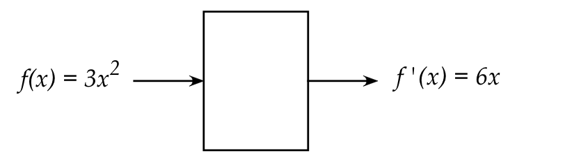
The box represents something that takes
as input a function and produces as output a function
\(\rhd\)
In this case, the derivative of the input function.
The idea of an operator:
- Whereas a function's input and output are numbers, we'll
use the term operator for action of taking a function
and returning a function.
- Our example showed the derivative operator.
- In notation, we'll write the derivative operator as
$$
{\bf D} \; f(x) \eql f^\prime(x)
$$
In other words, the operator \({\bf D}\) applied to the
function \(f(x)\) produces its derivative \(f^\prime(x)\)
as output.
- Clearly, one can imagine and design all kinds of operators.
- For example, here's a simple one: \({\bf S}_\alpha\)
is the scalar operator that multiples a function by the
number \(\alpha\):
$$
{\bf S}_\alpha \; f(x) \eql \alpha f(x)
$$
- This idea of the input/output being something other
than a number is one we've seen before with vectors:
$$
{\bf A} \; {\bf x} \eql {\bf y}
$$
Here, one can think of the effect of left-multiplying by
matrix \({\bf A}\) as:
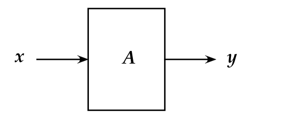
- The notation resembles our just-introduced operator notation
as well.
- Accordingly, we'll broaden our definition of operator to
apply both to functions and vectors, with the same notation:
$$\eqb{
{\bf D} \; f(x) & \eql & f^\prime(x)
& \;\;\;\;\;\;\;\mbox{Functions}\\
{\bf A} \; {\bf x} & \eql & {\bf y}
& \;\;\;\;\;\;\;\mbox{Vectors}
}$$
- Why is this useful?
- We will later see that a function can be thought of as
a "continuous" version of a vector.
- Thus, when transforming one function to another, we'll
extend the "multiply by a matrix on the left"
to "apply an operator on the left".
- What is interesting is that a general theory of operators
applies both to vectors and functions.
- Quantum mechanics makes significant use such operators.
- For example, the multiply-by-scalar operator can be
written to apply to either functions or vectors:
$$\eqb{
{\bf S}_\alpha \; \kt{f(x)} & \eql & \alpha \kt{f(x)}
& \;\;\;\;\;\;\;\mbox{Functions}\\
{\bf S}_\alpha \; \kt{\bf x} & \eql & \alpha \kt{\bf x}
& \;\;\;\;\;\;\;\mbox{Vectors}
}$$
- In the quantum literature, it's common to not distinguish
and use a single symbol like \(\pss\)
$$
{\bf S}_\alpha \; \kt{\pss} \eql \alpha \kt{\pss}
\;\;\;\;\;\;\;\mbox{Function or vector}
$$
- We'll later see that \(\pss\) is a unifying way to
refer to the state of a system
whether discrete (vector) or continuous (function).
- And an operator's effect will be analyzed using its eigenvectors
and eigenvalues, whether discrete (matrix) or continuous (operator).
\(\rhd\)
This will turn out to be the key to understanding the quantum world.
A point about notation:
- We've introduced notation for function operators like
\({\bf D} \; f(x) \eql f^\prime(x)\)
to see that it's similar to vector operators
\({\bf A} \; {\bf x} \eql {\bf y}\).
- But just as often, one peels back \(\frac{d}{dx}\)
from \(\frac{df}{dx}\) and treat \({\bf \frac{d}{dx}}\)
as an operator:
$$
{\bf \frac{d}{dx}} \; f(x) \eql f^\prime(x)
$$
- As an example, one could define the operator
\(
\left(
\frac{\partial^2}{\partial x^2}
-
\frac{1}{v^2}
\frac{\partial^2}{\partial t^2}
\right)
\)
and apply it to a function \(f(x,t)\):
$$
\left(
\frac{\partial^2}{\partial x^2}
-
\frac{1}{v^2}
\frac{\partial^2}{\partial t^2}
\right)
\;
f(x,t)
\eql
\frac{\partial^2 f(x,t)}{\partial x^2}
-
\frac{1}{v^2}
\frac{\partial^2 f(x,t)}{\partial t^2}
$$
Operators with "nice" properties:
- There are four properties that turn out to be critical when
considering operators: linear, Hermitian, unitary, bounded.
- A general operator \({\bf A}\),
whether a function operator or vector operator,
is linear if:
- For vector operator \({\bf A}\) and vectors
\({\bf x}\) and \({\bf y}\)
it's true that
$$
{\bf A}\; (\alpha {\bf x} + \beta {\bf y}) \eql
\alpha {\bf Ax} + \beta {\bf Ay}
$$
for all scalars \(\alpha, \beta\).
- For function operator \({\bf A}\) and functions
\(f\) and \(g\)
it's true that
$$
{\bf A}\; (\alpha f + \beta g) \eql
\alpha {\bf A}f + \beta {\bf A}g
$$
for all scalars \(\alpha, \beta\).
- As an example, consider the function operator
\({\bf \frac{d^2}{dx^2}}\) (the second derivative):
- This is a linear operator because
$$
{ \frac{d^2}{dx^2}} \; (\alpha f + \beta g) \eql
\alpha \frac{d^2}{dx^2}f + \beta \frac{d^2}{dx^2}g
$$
- For example, if \(f(x) = 3x^2, \; g(x)=e^{10x}\),
$$\eqb{
{\frac{d^2}{dx^2}} \; (\alpha f + \beta g)
& \eql &
{ \frac{d^2}{dx^2}} \; (\alpha 3x^2 + \beta e^{10x} ) \\
& \eql &
\alpha \frac{d^2}{dx^2} 3x^2 \;+ \; \beta \frac{d^2}{dx^2}e^{10x}\\
& \eql &
\alpha \frac{d^2}{dx^2}f + \beta \frac{d^2}{dx^2}g
}$$
- Generally, anything linear is easier to work with than
anything nonlinear, but the biggest significance is
in interpreting the linearity above:
- Suppose we have some linear differential equation like
$$
\frac{\partial^2 f(x,t)}{\partial x^2}
\eql
\frac{1}{v^2}
\frac{\partial^2 f(x,t)}{\partial t^2}
$$
- We notice that, in linear operator form, it can be written as:
$$
\left(
\frac{\partial^2}{\partial x^2}
-
\frac{1}{v^2}
\frac{\partial^2}{\partial t^2}
\right)
\;
f(x,t)
\eql
0
$$
- Since the operator is linear, if functions \(g(x,t)\) and
\(h(x,t)\) happen to be solutions to the equation, so is
any \(\alpha g(x,t) + \beta h(x,t) \).
- In this particular case, you can work through and show
that \(\sin(x - vt)\) and \(\cos(x - vt)\) are solutions, which
means \(A \sin(x - vt) + B \cos(x - vt)\) is a solution.
- In an actual application of the differential equation
there will be other constraints (called boundary conditions)
that need to be satisfied.
- For example: the value at \(t=0\) is \(0\).
- Then one applies these conditions to solve for the
constants \(A\) and \(B\), which then provide the actual
solution for the problem at hand.
- Not only is this useful for a particular problem, it
turns out to be theoretically critical since many key
features of the quantum world (quantization) arise through this.
- The next two properties depend on understanding complex vectors
and matricies, which we will cover in the course. For now, we'll just
list these properties.
- The second property is whether an operator
is Hermitian:
- A complex matrix (and therefore operator) \({\bf A}\)
is Hermitian if \({\bf A}^\dagger = {\bf A}\),
where \({\bf A}^\dagger\) is the conjugated transpose.
- An equivalent definition for function operators needs
more background, which we will defer to later.
- The third property is unitarity, whether the
operator is unitary or not.
- A complex matrix (and therefore operator) \({\bf A}\)
is unitary if \({\bf A}^\dagger = {\bf A}^{-1}\),
where \({\bf A}^\dagger\) is the conjugated transpose.
- Unitary operators are how we build quantum computations.
- The fourth property is boundedness, which we will also
defer, except to note that all matrix operators are bounded.
- Of these, the first three matter in quantum computing
but the fourth also matters in quantum mechanics.
- One of the key results to come from the first two properties is
that eigenvectors are orthogonal, and eigenvalues are real (no
imaginary part).
\(\rhd\)
These eigenvectors (and eigenvalues) are the essence of any
quantum system.
We will learn more about this topic later.
M.6 Waves and wavefunctions
First, we point out: nothing in this section is needed for the
course; it's here to stimulate curiosity.
Let's start this section with the obvious questions:
what do we mean by a "wave", and what does it have to do
with quantum computing?
We'll first address the second question:
- Waves are not really needed for most of quantum
computing.
- One particular formulation of quantum computing,
adiabatic quantum computing,
along with its particular hardware, does need a bit of "wave" background
to understand.
- But most importantly, for the curious,
we'll present a bit of background on quantum mechanics:
this will feature Schrodinger's equation, which is about a type
of "wave" (ominous quotes intended).
- And, here, an understanding of waves will reveal
one of the most startling and counter-intuitive
aspects of the quantum world:
- In the macroworld of big objects, a mathematical
wave (a differential equation)
describes a real physical wave, like a sound wave
or a pond ripple.
- Thus, there's some physical thing that's doing the "waving".
- However, in the quantum world, there is no physical
thing that "waves". Instead, most peculiarly, what does the
"waving" are probabilities that make the physical phenomena
random.
- This will take some background to explain - we'll get there
in time.
- Also, waves are generally useful to learn about
because you might one day decide to dig deeper into
quantum technologies or optics.
Let's start with some physical phenomena:
- The most commonly visible wave is probably some kind of water
wave, like ripples from a pebble dropped in a pond:
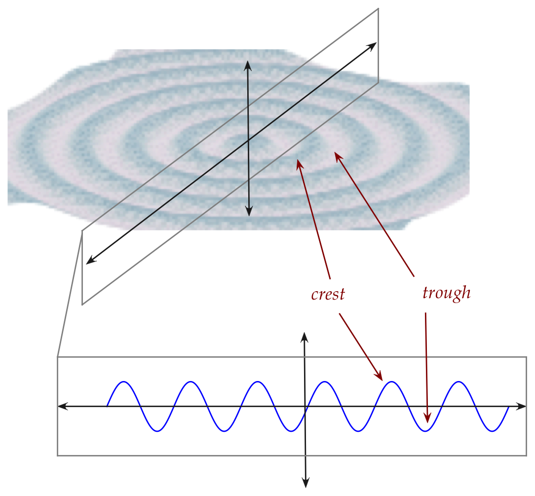
- To simplify, we'll look at a cross section.
- Notice: a particular water molecule doesn't actually move
away from the center, just up and down.
- This is called a transverse wave, where
the wave movement is perpendicular to the matter that moves.
- Consider a particular water molecule on the surface, some
distance from the center:
- This molecule moves up and down (strictly vertically).
- Think of this as away and towards its mean position.
- At some particular time, it will be at its highest position
\(\rhd\)
maximum positive displacement, a crest.
- At some later time, it will be at the lowest position
vertically
\(\rhd\)
maximum negative displacement, a trough.
- Suppose \(x\) describes position (distance) away from
the center, and \(t\) is time.
- Let \(f(x,t)\) = the displacement at position \(x\) at
time \(t\).
- For a fixed time \(t\), if we observe displacement along
\(x\), it will vary up and down.
- For a fixed position \(x\), if we observe the change in time,
again, there will be an up and down repetition.
\(\rhd\)
Both are similar!
- Another kind of wave comes from sound:
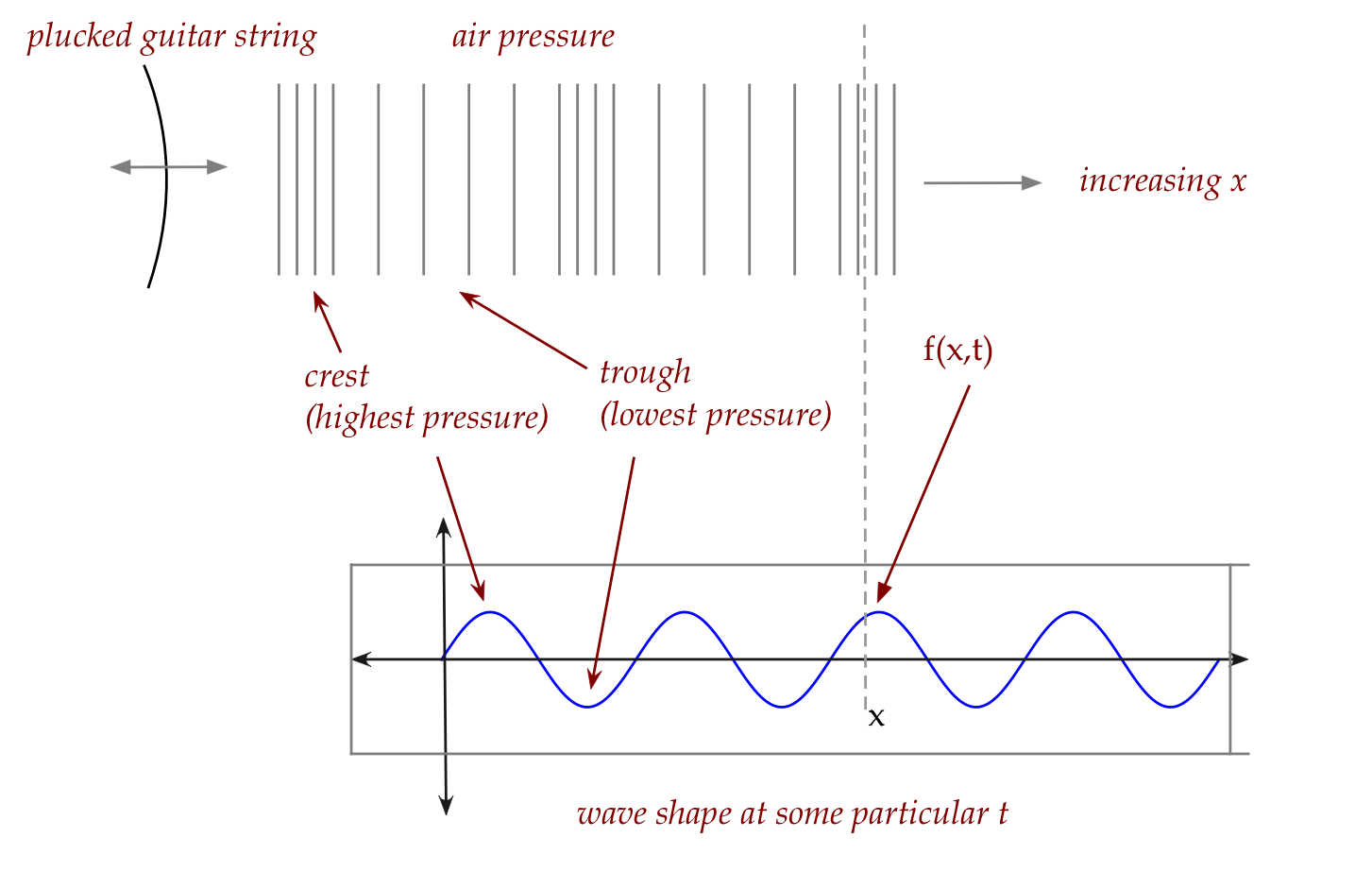
- It's harder to "see" the wave here.
- Note: matter moves in the same direction as the wave
\(\rhd\)
This type is called a longitudinal wave.
- Again, we observe similar shapes for changing \(t\) with fixed
\(x\) and for changing \(x\) for fixed \(t\).
- A more artificial, lab-suited wave:
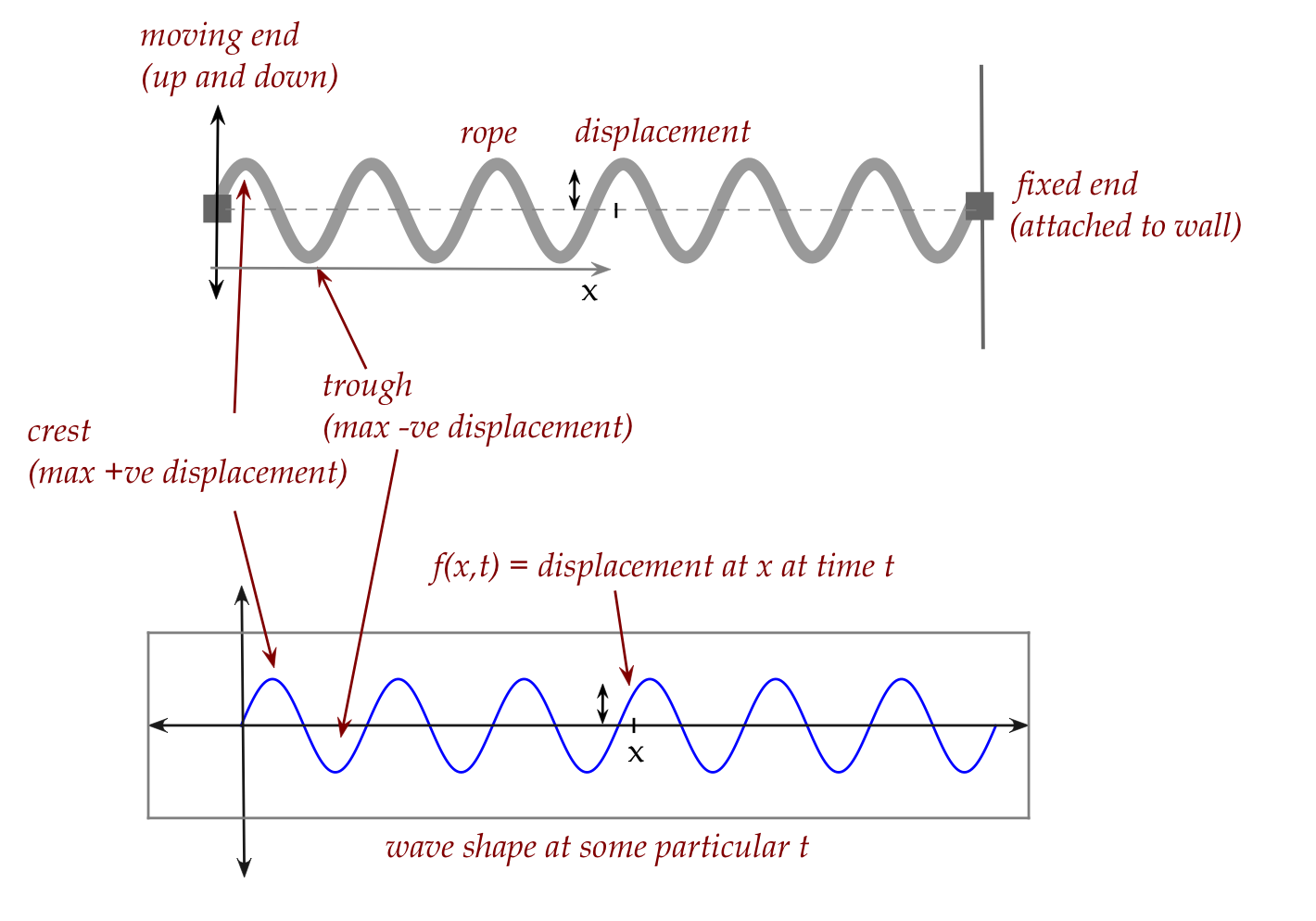
- One end (the right) of a rope is attached to a wall.
- The other end is moved up and down.
- This will cause the rope to exhibit a wave like shape.
The wave equation:
- We'll now, to simplify, make a uniformity assumption: that
the disturbance pattern is the same everywhere and continues
indefinitely.
- With uniformity, let's examine how \(f(x,t)\) looks at two different
\(x\) values:
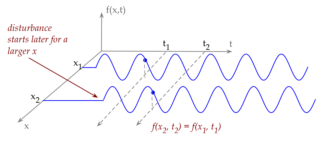
- These are examples of how \(f(x,t)\) changes with \(t\)
for fixed \(x\).
- Consider the value of \(f(x_2,t_2)\).
- Since the wave moved rightwards, this value must have
been at a previous \(x_1\) at an earlier time \(t_1\).
- If the wave velocity is \(v\) then
\(x_2 = x_1 + v(t_2 - t_1)\).
- Thus, \(f(x_2,t_2) = f(x_2 - v(t_2-t_1), t_1)\).
- Let's set \(t_1 = 0\) to make an observation:
\(f(x_2,t_2) = f(x_2 - v t_2, 0)\).
- Now for the key observation: the value of f at these
two x-values will be the same no matter what \(t_2\) is.
- Now define a new function \(h(x)\) to reflect this
equality: \(f(x,t) = h(x-vt)\).
- Think of \(h\) as the 'shape' function.
- With this, a few steps of applying partial derivatives shows
that
$$
\frac{\partial^2 f(x,t)}{\partial x^2}
\eql
\frac{1}{v^2}
\frac{\partial^2 f(x,t)}{\partial t^2}
$$
This is called the (one dimensional) wave equation.
- One can derive the wave equation from physical principles
(for example, rope tension, forces, and acceleration), with
some assumptions.
- The wave equation is quite general and broadly used in
many applications.
Solutions to the wave equation:
- Solutions to the wave equation are inevitably some form
of sinusoid, or more frequently, linear combinations of them.
- For example:
$$
f(x,t) \eql A \sin(\omega(x-vt)) + B \cos(\omega(x-vt))
$$
- One important variation is:
$$
f(x,t) \eql A \sin(kx - \omega t) + B \cos(kx - \omega t)
$$
where the parameters \(k\) and \(\omega\) turn out to have
physical meaning:
- The argument to a sinusoid is always an angle,
as in \(\sin(\theta)\).
- This 'angle' argument to a sinusoid is often called the phase.
- Here, \(k\) is a parameter that converts \(x\) into phase
(\(k\) is a sort of phase-to-distance ratio).
- And \(\omega\) is a time-to-angle converter called frequency.
\(\rhd\)
A higher frequency results in the phase changing more quickly.
\(\rhd\)
Which means more cycles per unit time.
- Perhaps the most important variation is the complex
version:
$$
f(x,t) \eql C e^{i(kx - \omega t)}
$$
- In case you were wondering about the negative sign in
\((kx - \omega t)\), this comes about with a rightward moving
wave (increasing x). When a move moves leftward we get
\((kx + \omega t)\), so the more general solution is sometimes
written as
$$
f(x,t) \eql C e^{i(kx \pm \omega t)}
$$
It will be useful to know what happens when waves 'encounter' other things,
especially, other waves:
Summary: why did we spend time on waves?
- There is an equation that's similar to the wave equation,
and whose solutions are also complex exponentials:
$$
i\hbar \frac{\partial f(x,t)}{\partial t}
\eql
- \frac{\hbar^2}{2m} \frac{\partial^2 f(x,t)}{\partial x^2}
+ V(x,t) \; f(x,t)
$$
- This is the famous Schrodinger equation, the
foundational equation of quantum mechanics.
- Even though the function \(f(x,t)\) is not really a wave
in the sense of what we've seen, it's called a wavefunction.
- The symbol \(\Psi\) is what's commonly used and the
equation is often written as:
$$\eqb{
i\hbar \frac{\partial \Psi(x,t)}{\partial t}
& \eql &
\left( - \frac{\hbar^2}{2m} \frac{\partial^2}{\partial x^2}
+ V \right) \Psi(x,t) \\
& \eql &
{\bf H} \; \Psi(x,t)
}$$
where the term in parenthesis is a linear operator \({\bf H}\) called
the Hamiltonian
- What is truly strange is that \(\Psi(x,t)\) indirectly represents
probabilities and these will vary in a wave-like manner.
- The strangest part of this strangeness is that such
\(\Psi(x,t)\) quantities can be added
much like we added waves to cause interference.
- Here's the surprising implication for quantum computing:
it is this interference, as we will see,
that actually forms the basis of many quantum computing algorithms.
- Note: it might be a relief to know that, in quantum computing,
everything is discrete, and we will not need Schrodinger's
equation at all.
\(\rhd\)
Instead, we'll be adding the scalars in linear combinations of vectors.
Back to main review page


