\(
\newcommand{\blah}{blah-blah-blah}
\newcommand{\eqb}[1]{\begin{eqnarray*}#1\end{eqnarray*}}
\newcommand{\eqbn}[1]{\begin{eqnarray}#1\end{eqnarray}}
\newcommand{\bb}[1]{\mathbf{#1}}
\newcommand{\mat}[1]{\begin{bmatrix}#1\end{bmatrix}}
\newcommand{\nchoose}[2]{\left(\begin{array}{c} #1 \\ #2 \end{array}\right)}
\newcommand{\defn}{\stackrel{\vartriangle}{=}}
\newcommand{\rvectwo}[2]{\left(\begin{array}{c} #1 \\ #2 \end{array}\right)}
\newcommand{\rvecthree}[3]{\left(\begin{array}{r} #1 \\ #2\\ #3\end{array}\right)}
\newcommand{\rvecdots}[3]{\left(\begin{array}{r} #1 \\ #2\\ \vdots\\ #3\end{array}\right)}
\newcommand{\vectwo}[2]{\left[\begin{array}{r} #1\\#2\end{array}\right]}
\newcommand{\vecthree}[3]{\left[\begin{array}{r} #1 \\ #2\\ #3\end{array}\right]}
\newcommand{\vecdots}[3]{\left[\begin{array}{r} #1 \\ #2\\ \vdots\\ #3\end{array}\right]}
\newcommand{\eql}{\;\; = \;\;}
\newcommand{\eqt}{& \;\; = \;\;&}
\newcommand{\dv}[2]{\frac{#1}{#2}}
\newcommand{\half}{\frac{1}{2}}
\newcommand{\mmod}{\!\!\! \mod}
\newcommand{\ops}{\;\; #1 \;\;}
\newcommand{\implies}{\Rightarrow\;\;\;\;\;\;\;\;\;\;\;\;}
\newcommand{\prob}[1]{\mbox{Pr}\left[ #1 \right]}
\newcommand{\probm}[1]{\mbox{Pr}\left[ \mbox{#1} \right]}
\newcommand{\simm}[1]{\sim\mbox{#1}}
\definecolor{dkblue}{RGB}{0,0,120}
\definecolor{dkred}{RGB}{120,0,0}
\definecolor{dkgreen}{RGB}{0,120,0}
\)
Module 7: Probability and Simulation
7.1 A sample application
A queueing simulation:
- Experiments like coin flips are easy to simulate
→ The simulation code is itself simple.
- The subject of simulation is concerned with more complex systems
→ Here, the simulation code itself may be intricate.
- Queueing systems are classic examples in simulation
→ Many simulation principles can be learned from these systems.
- Consider a simple two-queue example:

- There are two service stations (kiosks).
Each station has a separate queue for customers.
- Customers arrive to the system from outside.
→ Their interarrival times are random.
- Each customer picks a queue to join and waits for service.
- The service time for each customer is random.
- Generally, we simulate for a purpose: to estimate something
- The average waiting time for a customer.
- Is it better for customers to select the shortest queue
or flip a coin to decide which queue to join?
Exercise 1:
Download, compile and execute QueueControl.java,.
setting animate=true and
clicking "reset" followed by "go".
(You will also need RandTool.java)
- You can step through and observe the sequence of events.
- Use animate=false and estimate the average wait time
for customers.
- What queue-selection policy are customers using? Change the
policy to improve the waiting time.
Elements of a simulation:
- Methods for generating randomness
e.g., random interarrivals and random service times.
- How to track time
e.g., advance the clock from one key point to the next.
- How to store key aspects and ignore inessential ones
e.g., store waiting customers, but not departed customers.
- How to record statistics
e.g., collect wait times at customer departure moments.
- What data structures are useful
e.g., a priority queue
Exercise 2:
Consider the time spent in the system by each customer.
The simulation computes the average "system time."
- Is this a discrete or continuous quantity?
- Are the system times of two successive customers independent?
Before learning how to write simulations, we will need to
understand a few core concepts in probability:
- Random variables and distributions.
- Expectation and laws of large numbers.
- Dependence, joint and conditional distributions.
- Statistics: how to estimate and know how many samples you need.
7.2 Random variables
A random variable is an observable numeric quantity from
an experiment:
- Coin flip example:
- "Heads" and "Tails" are not numeric, but 1 and 0 are.
- For multiple coin flips, one can count the number of heads.
- More coin-flip related random variables:
- How many flips does it take to get two heads in a row?
Random variable: number of such flips
- How many heads in 10 coin flips?
Random variable: number of heads
- Dice example:
- Sum of numbers that show up in two rolls
Random variable: the sum
- Bus-stop example:
- How long before the next bus arrives?
Random variable: actual waiting time
- How many buses arrive in a 10-minute period?
Random variable: number of such buses.
Exercise 3:
Identify some random variables of
interest in the Queueing example.
Range of a random variable: the possible values it can take
- Example: number of heads in 10 flips
\(\Rightarrow\) range = \(\{0,1,2,...,10\}\)
- Example: sum of two dice
\(\Rightarrow\) range = \(\{2,3,...,12\}\)
Exercise 4:
What are the ranges for these random variables?
- The number of buses that arrive in a 10-minute period.
- The waiting time for the next bus to arrive.
Notation
- Sometimes we use the short form rv = random variable.
- Typically, we use capital letters to denote rv's:
- Let \(X = \) number of heads in 10 coin flips.
- Let \(Y = \) the waiting time for the next bus to arrive.
Let's look at the \(n\)-coin flip example in more detail:
- Let \(X = \) number of heads in \(n\) coin flips.
- Suppose \(\probm{heads} = 0.6\) for a single flip.
- Consider the events when \(n=3\) (3 flips)
| Outcome | \(\probm{outcome}\) | value of \(X\) |
| \(HHH\) | 0.6 * 0.6 * 0.6 | \(X = 3\) |
| \(HHT\) | 0.6 * 0.6 * 0.4 | \(X = 2\) |
| \(HTH\) | 0.6 * 0.4 * 0.6 | \(X = 2\) |
| \(HTT\) | 0.6 * 0.4 * 0.4 | \(X = 1\) |
| \(THH\) | 0.4 * 0.6 * 0.6 | \(X = 2\) |
| \(THT\) | 0.4 * 0.6 * 0.4 | \(X = 1\) |
| \(TTH\) | 0.4 * 0.4 * 0.6 | \(X = 1\) |
| \(TTT\) | 0.4 * 0.4 * 0.4 | \(X = 0\) |
- First, note:
- We've assumed independence between coin flips
e.g., \(\probm{HHT}\) = Pr[1st is heads] * Pr[2nd is heads] * Pr[3rd is tails]
- Each individual outcomes results in an observable numeric value for the rv of interest (\(X\)).
- Notice the following
- The range of \(X\) is \(X \in \{0,1,2,3\}\).
- \(\prob{X = 3} \eql \probm{HHH} \eql 0.6 * 0.6 * 0.6 \eql 0.216\)
- \(\prob{X = 0} \eql \probm{TTT} \eql 0.4 * 0.4 * 0.4 \eql 0.064\)
- The two remaining probabilities of interest are:
\(\prob{X=1}\) and \(\prob{X=2}\)
- \(\prob{X=1} \eql \probm{HTT} + \probm{THT} + \probm{TTH} \eql 3 * 0.4 * 0.6 *0.4 \eql 0.288\)
- \(\prob{X=2} \eql \probm{HHT} + \probm{HTH} + \probm{THH} \eql 3 * 0.6 * 0.6 *0.4 \eql 0.432\)
- We've made use of Axiom 3 (disjoint events).
- Thus, this list is complete for \(X\):
\(\prob{X=0} \eql 0.064\)
\(\prob{X=1} \eql 0.288\)
\(\prob{X=2} \eql 0.432\)
\(\prob{X=3} \eql 0.216\)
- Clearly,
\(\prob{X=0} + \prob{X=1} + \prob{X=2} + \prob{X=3} \eql 1\)
Exercise 5:
What is \(\prob{X \leq 2}\) above? Write down \(\prob{X \leq k}\)
for all relevant values of \(k\).
Next, suppose \(\probm{heads} = p\) in the above example. Write
down \(\prob{X=i}, i\in \{0,1,2,3\},\) in terms of \(p\).
Discrete vs. continuous random variables:
- Discrete: when the range is finite or countably infinite.
- Continuous: when the range is real-valued.
- To specify probabilities for a discrete rv \(X\), we need to
specify \(\prob{X=k}\) for every possible value \(k\).
- For continuous rv's it's a little more complicated
\(\Rightarrow\) We will get to this later.
- This specification of probabilities is called a distribution.
7.3 Discrete distributions
Consider the following rv and distribution:
- Random variable \(X\) has range \(\{0,1\}\).
- Thus, one needs to specify
\(\prob{X=0} = ?\)
\(\prob{X=1} = ?\)
- For example,
\(\prob{X=0} = 0.4\)
\(\prob{X=1} = 0.6\)
- One application is coin tossing: \(X=1\) (heads) or
\(X=0\) (tails).
- This type of rv can be used for any success-failure type of
experiment where \(0=\mbox{failure}\) and \(1=\mbox{success}\).
- In general, we write this type of distribution as
\(\prob{X=0} = 1-p\)
\(\prob{X=1} = p\)
where \(p\) is the success probability.
- This type of rv is called a Bernoulli rv.
- The associated distribution is called a Bernoulli distribution.
- Here \(p\) is called a parameter of the distribution.
\(\Rightarrow\) In a particular problem, \(p\) would have
some value like \(p=0.6\).
- Note: \(\prob{X=0} + \prob{X=1} = 1\), as we would expect.
To summarize:
- A discrete rv \(X\) takes on values in some set \(A\)
where \(A\) is finite or countably infinite.
- Probabilities are specified by giving \(\prob{X=k}\) for
each \(k \in A\).
- This list of probabilities is called the distribution of \(X\).
- Because some distributions are used for multiple purposes,
we often parameterize them to study general properties.
It is now possible to work with distributions in the abstract
without specifying an experiment.
- For the distribution to be valid, those probabilities should
sum to 1.
$$
\sum_{k} \prob{X=k} \eql 1
$$
Exercise 6:
What would be an example of a discrete rv
in the Queueing application?
An example of a distribution (in the abstract):
- Consider a rv \(X\) with range \(\{1,2,...\}\).
- Suppose the distribution of \(X\) is given by
$$
\prob{X=k} \eql (1-p)^{k-1} p
$$
where \(p\) is a parameter such that \(0 \lt p \lt 1\).
- Here are a few sample values:
\(\prob{X=1} = p\)
\(\prob{X=2} = (1-p) p\)
\(\prob{X=3} = (1-p)^2 p\)
\(\vdots\)
- This distribution is called the Geometric distribution.
- Note: this distribution has one parameter (\(p\)).
- We use the short form
\(X \sim \mbox{Geometric}(p)\)
to mean
"rv \(X\) has the Geometric distribution with parameter \(p\)"
- One application: coin flips
Let \(X = \) the number of flips needed to get the first heads.
\(\Rightarrow\) \(\prob{X=k} = \probm{k-1 tails in a row, then heads}\)
\(\Rightarrow\) \(\prob{X=k} = \probm{tails} \probm{tails}
\mbox{... (k-1) times ... } \probm{tails} \probm{heads}\)
\(\Rightarrow\)
\(\prob{X=k} = (1-p)^{k-1} p\)
Exercise 7:
Verify by hand that
\(\sum_k \prob{X=k} = 1\)
for the above distribution.
Exercise 8:
If \(p=0.6\), what is the probability that the first heads appears
on the 3rd flip? Verify your answer using Coin.java
and CoinExample.java.
Exercise 9:
Suppose I compare two parameter values for the Geometric distribution:
\(p=0.6\) and \(p=0.8\).
For which of the two values of \(p\) is \(\prob{X=3}\) higher?
Exercise 10:
Compute (by hand) \(\prob{X\gt k}\) when \(X\sim\mbox{Geometric}(p)\).
The discrete uniform distribution:
- A rv \(X\) has the discrete uniform distribution if:
- It has a finite range, i.e., \(X \in A\) where
\(|A|\) is finite.
- And $$\prob{X=k} \eql \frac{1}{|A|}$$
- Example: die roll
- Range is finite: \(X \in \{1,2,...,6\}\).
- \(\prob{X=k} = \frac{1}{6}\).
- Example: card drawing.
- Range is finite: \(X \in \{0,1,2,...,51\}\).
- \(\prob{X=k} = \frac{1}{52}\).
- Quite often, useful discrete-uniform rv's have a range
of \(\{0,1,...,m-1\}\) or \(\{1,2,...,m\}\).
In the latter case, we write \(X\sim\mbox{Discrete-uniform}(1,m)\).
The Binomial distribution:
- A rv \(X\) has the Binomial distribution with parameters
\(n\) and \(p\) (two parameters) if:
- \(X\) has range \(\{0,1,...,n\}\).
- And
$$ \prob{X=k} \eql \nchoose{n}{k} p^k (1-p)^{n-k} $$
- Short form: \(X\simm{Binomial}(n,p)\).
- Example: coin flips
- A coin with \(\prob{H} = p\) is flipped \(n\) times.
- \(X\) counts the number of heads.
- To see why this is appropriate for coin flips:
- Suppose we want to compute \(\prob{X=k}\)
\(\Rightarrow\) Probability of observing exactly \(k\) heads.
- Think of the \(n\) flips as a string over the alphabet \(\{H,T\}\).
e.g. HHTTH = 3 heads in 5 flips
- Now consider \(k\) heads in \(n\) flips:

- The probability of getting exactly \(k\) heads and
exactly \((n-k)\) tails is:
\(p^k (1-p)^{n-k}\)
- But there are \(\nchoose{n}{k}\) ("n choose k") different
ways of arranging the \(k\) heads.
\(\Rightarrow\) Each is a possible outcome
\(\Rightarrow\)
\(\prob{X=k} \eql \nchoose{n}{k} p^k (1-p)^{n-k} \)
Exercise 11:
Suppose we flip a coin \(n\) times and count the number of heads using
a coin for which \(\prob{H} = p\).
- Write code to compute \(\prob{X=k}\) using the formula
\(\prob{X=k} \eql \nchoose{n}{k} p^k (1-p)^{n-k} \)
Write your code in Binomial.java.
- Plot a graph of \(\prob{X=k}\) vs. \(k\) for the case
\(n=10, p=0.6\) and for the case \(n=10, p=0.2\).
- Write a simulation to estimate \(\prob{X=3}\) when \(n=10, p=0.6\).
You can use Coin.java
and CoinExample2.java for
this purpose. Verify the estimate using the earlier formula.
Exercise 12:
For the above experiment, verify that the sum of probabilities
is 1. How would you prove this analytically for the Binomial distribution?
The Poisson distribution:
- \(X\simm{Poisson}(\gamma)\) if:
- \(X\) has range \(\{0,1,2,...\}\)
- And
$$\prob{X=k} \eql e^{-\gamma}\frac{\gamma^k}{k!}$$
- Thus, the Poisson rv counts zero or more occurences when the
number of possible occurences can be arbitrarily large.
\(\Rightarrow\)Unlike the number of heads in a fixed number of flips.
- Note: this distribution has only one parameter (\(\gamma\)).
- An application? It turns out that "the number of buses that
arrive in a fixed interval" is a good application.
\(\Rightarrow\) Why this is so is not trivial to show.
Exercise 13:
Add code to Poisson.java to
compute \(\prob{X=k}\) and plot a graph of \(\prob{X=k}\) vs. \(k\)
when \(\gamma=2\).
Use the Taylor series for \(e^x\) to
prove that \(\sum_k \prob{X=k}\) adds up to 1.
Exercise 14:
Download BusStop.java and
BusStopExample3.java,
and modify the latter to estimate the probability that exactly three
buses arrive during the interval \([0,2]\).
Compare this with \(\prob{X=3}\) when \(X\simm{Poisson}(2)\).
7.4 The cumulative distribution function (CDF)
Consider \(X\simm{Binomial}(n,p)\):
- We know that \(X\)'s range is \(\{0,1,...,n\}\) and that
the distribution specifies \(\prob{X=k}\).
- Now consider the probability \(\prob{X \leq y}\) for some
number \(y\).
- Example: \(\prob{X \leq 5}\)
- In this case:
$$
\prob{X \leq 5} \eql \prob{X=0} + \prob{X=1} + \ldots +
\prob{X=5}
$$
Exercise 15:
Plot \(\prob{X \leq k}\) vs \(k\) for \(X\simm{Binomial}(10,0.6)\).
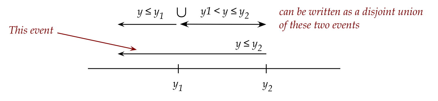
- Next, observe that
$$\eqb{
\prob{X \leq 5} & \eql & \prob{X=0} + \prob{X=1} +
\prob{X=3} \\
& & + \prob{X=4} + \prob{X=5} \\
& \eql & \prob{X \leq 3} \;\; + \;\; \prob{3 \lt X \leq 5}
}$$
- In general, for \(m \lt k\)
\(\prob{X \leq k} = \prob{X \leq m} + \prob{m \lt X \leq k}\)
- Now, consider \(\prob{X \leq 5.32}\) when \(X\simm{Binomial}(n,p)\).
Does this make sense?
- It can if we write
$$\prob{X \leq 5.32} \eql \prob{X \leq 5} + \prob{5 \lt X
\leq 5.32}$$
- Obviously, \(\prob{5 \lt X \leq 5.32} = 0\)
\(\Rightarrow\) \(\prob{X \leq 5.32} = \prob{X \leq 5}\).
- In this way, \(\prob{X \leq y}\) is well defined for any
value of \(y\).
- Since it is defined for every \(y\), it is a
function of \(y\):
\(F(y) \eql \prob{X \leq y}\)
\(\Rightarrow\) called the Cumulative Distribution Function (CDF)
of rv \(X\)

- CDFs are usually defined for all possible \(y\):
\(y \in (-\infty, +\infty)\)
- Important: When we write \(F(y)\) do NOT think of
\(y\) as the "y" axis. Instead: it's just an argument (input) to the
function \(F\). In fact, when we plot \(F(y)\) vs \(y\), then \(y\)
will be on the horizonal axis, while \(F(y)\) will be on the vertical axis.
Exercise 16:
Plot (by hand, on paper) the CDF \(F(y)\) for \(X\simm{Bernoulli}(0.6)\).
Next, consider the sequence of real numbers
\(y_n = (1 - \frac{1}{n})\)
and the sequence
\(z_n = (1 + \frac{1}{n})\)
Compute by hand or by programming the following limits:
- \(lim_{n\to\infty} y_n\)
- \(lim_{n\to\infty} z_n\)
- \(lim_{n\to\infty} F(y_n)\)
- \(lim_{n\to\infty} F(z_n)\)
What do you notice?
About the CDF for discrete rv's:
- The CDF is right-continuous
You can approach \(F(y)\) from the right, but not always
from the left.
- The CDF \(F(y)\) never decreases with increasing \(y\).
Exercise 17:
Why is this true?
Exercise 18:
Suppose rv \(X\) denotes the outcome (\(\{1,2,...,6\}\)) of
a die roll. Draw by hand the CDF.
Exercise 19:
Consider the distribution for the 3-coin-flip example:
\(\prob{X=0} = 0.064\)
\(\prob{X=1} = 0.288\)
\(\prob{X=2} = 0.432\)
\(\prob{X=3} = 0.216\)
Sketch the CDF on paper.
Exercise 20:
For the two CDFs we've seen so far (Bernoulli, Discrete-Uniform), is
it possible to differentiate the function \(F(y)\)? If so, what
is the derivative for the Bernoulli case?
Consider a CDF \(F(y)\) of a rv \(X\):
Exercise 21:
Suppose \(X\simm{Geometric}(p)\).
- Argue that \(\prob{X\gt k} = (1-p)^k\).
- Then write down the CDF.
- Write down an expression for \(\prob{3.11 \lt X \leq 5.43}\) in
terms of the CDF.
7.5 Continuous random variables
Exercise 22:
Recall the Bus-stop example. Suppose rv \(X\) denotes
the first interarrival time. Download
BusStop.java,
RandTool.java,
and
BusStopExample.java.
Then modify the latter to estimate the following:
- \(\prob{X \lt 1}\)
- \(\prob{X \lt 1.1}\)
- \(\prob{X=1}\)
Exercise 23:
What is an example of a continuous rv associated
with the QueueControl.java
application?
The difficulty with continuous rv's:
- First, \(\prob{X=x} = 0\) for most continuous rv's \(X\).
\(\Rightarrow\) This means we can't specify the distribution using a list.
- Second, it's not clear how we can get probabilities to sum
to 1.
e.g., for a rv that takes any real value in \([0,1]\), how
do we sum probabilities?
- Fortunately, the CDF offers a way out.
Let's write some code to estimate a CDF:
- First, identify the range \([a,b]\) of interest.
- Then, break this up into \(M\) small intervals:
\([a,a+\delta ], [a+\delta ,a+2\delta ], \ldots, [a+(M-1)\delta ,a+M\delta ]\)
- Maintain a counter intervalCount[i] for each interval.
- For any random value \(x\), identify the interval
\(j = \lfloor \frac{x-a}{\delta} \rfloor \)
and increment the count of every interval \(i \geq j\).

- Pseudocode:
    Algorithm: cdfEstimation (M, a, b)
    Input: number of intervals M, range [a,b]
    1.   δ = (b-a) / M
    2.   for n=1 to numTrials
    3.       x = generateRV ()
    4.       j = floor ( (x-a) / δ )
    5.       for i=j to M-1
    6.           intervalCount[i] = intervalCount[i] + 1
    7.       endfor
    8.   endfor
         // Now build and print the CDF
    9.   for i=0 to M-1
    10.      midPoint = a + iδ + δ/2                           // Interval: [a+iδ,a+(i+1)δ]
    11.      print (midPoint, intervalCount[i] / numTrials)
    12.  endfor
- Sample code:
(source file)
    static Function makeUniformCDF ()
    {
	double a = 0, b = 1;
	int M = 50;                   // Number of intervals.
	double delta = (b-a) / M;     // Interval size.

	double[] intervalCounts = new double [M];
	double numTrials = 1000000;

	for (int t=0; t<numTrials; t++) {
            // Random sample:
	    double y = RandTool.uniform ();
            // Find the right interval:
            int k = (int) Math.floor ((y-a) / delta);
            // Increment the count for every interval above and including k.
            for (int i=k; i<M; i++) {
                intervalCounts[i] ++;
            }
	}

	// Now compute probabilities for each interval.
	double[] cdf = new double [M];
	for (int k=0; k<M; k++) {
	    cdf[k] = intervalCounts[k] / numTrials;
	}

        // Build the CDF. Use mid-point of each interval.
        Function F = new Function ("Uniform cdf");
	for (int k=0; k<M; k++) {
	    double midPoint = a + k * delta + delta/2;
            F.add (midPoint, cdf[k]);
	}

        return F;
    }
Exercise 24:
Download and execute UniformCDF.java.
You will also
need Function.java,
RandTool.java,
and
SimplePlotPanel.java.
Modify the code to print \(F(1)-F(0.75)\).
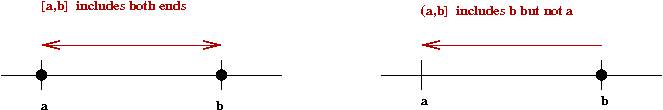
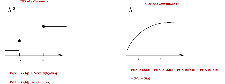
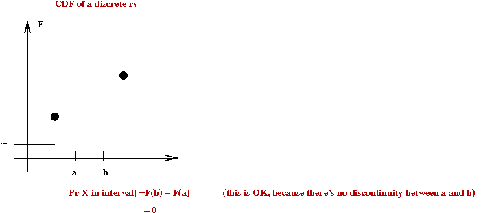
Getting probabilities out of a CDF:
- Recall that for any rv \(X\) with CDF \(F\):
\(\prob{y_1 \lt X \leq y_2}
= F(y_2) - F(y_1)\)
- Thus, for example, if \(X\) has the uniform CDF
\(\prob{0.75 \lt X \leq 1.0}
= F(1) - F(0.75)\)
- Important: the CDF gets you the probability that
\(X\)'s outcome lands in any particular interval of interest:
\(\probm{X falls in any interval (a,b]} = F(b) - F(a)\)
Exercise 25:
The program GaussianCDF.java
estimates the CDF of a Gaussian rv. Execute the program
to plot the CDF. Then, use this CDF to compute the following probabilities:
- \(\prob{0 \lt X \leq 2}\).
- \(\prob{X \gt 0}\).
A small technicality that goes to the heart of a continuous rv:
Exercise 26:
Modify UniformCDF.java
and GaussianCDF.java
to compute the derivative of each. What is the shape of \(F'(y)\)
in each case?
Exercise 27:
If \(X\) denotes the first interarrival time in the bus-stop
problem, estimate the CDF of \(X\) as follows:
- Assume that values fall in the range \([0,3]\) (i.e.,
disregard values outside this range).
- Use ExponentialCDF.java
as a template, and add modified code from
UniformCDF.java
- Next, compute the derivative of this function and
display it.
About CDFs and derivatives:
- The concept of CDF applies to both discrete and continuous rv's.
- The CDF of a discrete rv is not differentiable.
- For continuous rv's, the derivative is called a
probability density function (pdf).
- The pdf has two uses:
- It's useful in some calculations as we'll see below.
- Most books use the pdf
\(\Rightarrow\) You need to be comfortable with the pdf to read them.
- For completeness, note that the list of probabilities for
a discrete rv is called a probability mass function
(pmf), e.g.
\(\prob{X=0} = 0.064\)
\(\prob{X=1} = 0.288\)
\(\prob{X=2} = 0.432\)
\(\prob{X=3} = 0.216\)
- Customarily, a discrete rv's distribution is specified by
giving its pmf.
\(\Rightarrow\) The CDF is not really useful for discrete rv's
- Customarily, a continuous rv's distribution is specified by
giving its pdf.
\(\Rightarrow\) The CDF is equivalent (because you can take its derivative to get the pdf)
- To summarize:
- Discrete rv's use a pmf.
- Continuous rv's use a pdf.
- Both use a CDF.
7.6 Expectation - the discrete case
The expected value of a rv is a calculation
performed on its distribution:
- If \(X\) is a discrete rv with range \(A\), then
$$
\mbox{Expected value of }X \eql \sum_{k\in A} k \; \prob{X=k}
$$
- We write this as
$$
E[X] \eql \sum_{k\in A} k \; \prob{X=k}
$$
- Note: this is merely a calculation, and (so far) has nothing
to do with the English word "expect".
- \(E[X]\) is a number (not a function).
- Example: recall the 3-coin-flip example where \(X\) =
number-of-heads (we'll use \(\prob{H}=0.6\)).
- The range: \(A = \{0,1,2,3\}\).
- The pmf:
\(\prob{X=0} = 0.064\)
\(\prob{X=1} = 0.288\)
\(\prob{X=2} = 0.432\)
\(\prob{X=3} = 0.216\)
- Thus,
$$\eqb{
E[X] & \eql & \sum_{k\in \{0,1,2,3\}} k \; \prob{X=k} \\
& \eql &
0 \; \prob{X=0} + 1 \; \prob{X=1} + 2 \; \prob{X=2} +
3\; \prob{X=3} \\
& \eql &
0*0.064 + 1*0.288 + 2*0.432 + 3*0.216
}$$
Exercise 28:
Complete the calculation above.
What would you get if \(\prob{H}=0.5\)?
A few more examples:
- \(X \simm{Bernoulli}(p)\)
- Recall the pmf:
\(\prob{X=0} = 1-p\)
\(\prob{X=1} = p\)
- Thus,
$$\eqb{
E[X] & \eql & 0 \; \prob{X=0} + 1\; \prob{X=1}\\
& \eql & 0*(1-p) + 1*p = p
}$$
- In particular, for a fair coin \(p=0.5\) and so \(E[X]=0.5\).
- \(X\simm{Geometric}(p)\)
- The range: \(X\in \{1,2,\ldots \}\)
- The pmf:
\(\prob{X=k} = (1-p)^{k-1} p\)
- Thus,
$$\eqb{
E[X] & \eql & \sum_{k=1}^\infty k \; \prob{X=k} \\
& \eql & \sum_{k=1}^\infty k (1-p)^{k-1} p \\
& \eql & \frac{1}{p}
}$$
- \(X \simm{Binomial}(n,p)\)
- The range: \(X \in \{0,1,2,...,n\}\)
- The pmf:
\(\prob{X=k} \eql \nchoose{n}{k} p^k (1-p)^{n-k} \)
- Thus,
$$\eqb{
E[X] & \eql & \sum_{k=0}^{n} k\; \prob{X=k} \\
& \eql & \sum_{k=0}^{n} k \nchoose{n}{k} p^k (1-p)^{n-k} \\
& \eql & np
}$$
(The last step is not at all obvious.)
Exercise 29:
How does this relate to the 3-coin-flip example?
- \(X\simm{Discrete-uniform}(1,k)\)
- The range: \(X\in \{1,2,...,m\}\)
- The pmf:
\(\prob{X=k} = \frac{1}{m}\)
- Thus,
$$\eqb{
E[X] & \eql & \sum_{k=1}^m k \; \prob{X=k} \\
& \eql & \sum_{k=1}^m k \frac{1}{m} \\
& \vdots & \\
& \eql & \frac{m+1}{2}
}$$
- \(X\simm{Poisson}(\gamma)\)
- The range: \(X\in \{0,1,2,...\}\)
- The pmf:
\(\prob{X=k} \eql e^{-\gamma}\frac{\gamma^k}{k!}\)
- Thus,
$$\eqb{
E[X] & \eql & \sum_{k=0}^\infty k \; \prob{X=k} \\
& \eql & \sum_{k=0}^\infty k e^{-\gamma}\frac{\gamma^k}{k!}\\
& \vdots & \\
& \eql & \gamma
}$$
Exercise 30:
Fill in the steps for the last two expectations (discrete-uniform, Poisson).
What is the meaning of this expected value?
- First, let's return to the 3-coin-flip example where
\(\prob{X=0} = 0.064\)
\(\prob{X=1} = 0.288\)
\(\prob{X=2} = 0.432\)
\(\prob{X=3} = 0.216\)
- Now suppose we perform \(n\) trials
Let \(n_0 = \)number of occurences of \(0\)
in the trials.
Similarly, let \(n_1 = \)number of occurences of \(1\)
in the trials.
... etc
- Next, let
\(S_n = \) the sum of values obtained.
- Notice that
\(\frac{1}{n} S_n = \) average of values obtained.
- For example, suppose we ran some trials and obtained
\(3, 1, 1, 0, 2, 0, 1, 2, 2, 2\)
In this case
\(n_0 = 2\)
\(n_1 = 3\)
\(n_2 = 4\)
\(n_3 = 1\)
\(S_n = 14\)
This is evident, if we group the values:
0, 0, 1, 1, 1, 2, 2, 2, 2, 3
- Next, notice that
\(S_n \eql 0 + 1*3 + 2*4 + 3*1\)
\(= 0*n_0 + 1*n_1 + 2*n_2 + 3*n_3 \)
\(= \sum_k k\; n_k\)
- Now consider the limit
$$\eqb{
\lim_{n\to\infty} \frac{1}{n} S_n
\eqt
\lim_{n\to\infty} \frac{1}{n} \sum_{k} k n_k \\
\eqt
\lim_{n\to\infty} \sum_{k} k\; \frac{n_k}{n} \\
}$$
Exercise 31:
What does \(\frac{n_k}{n}\) become in the limit?
Unfold the sum for the 3-coin-flip example to see why this is true.
- Thus,
$$\eqb{
\lim_{n\to\infty} \frac{1}{n} S_n
\eqt
\sum_{k} k\; \prob{X=k} \\
\eqt
E[X]
}$$
- Thus, even though \(E[X]\) is a calculation done with the
distribution, it turns out to be the average (mean) outcome in the
long run (limit).
(provided of course we believe \(\frac{n_k}{n}\to \prob{X=k}\)).
Exercise 32:
Download Coin.java and
CoinExample3.java
and let \(X=\) the number of heads in 3 coin flips.
- Compute the average value of \(X\) using
\(\frac{1}{n} S_n\)
- Estimate \(\prob{X=k}\) using \(\frac{n_k}{n}\).
- Compute \(\sum_{k} k\; \frac{n_k}{n}\) using the estimates
of \(\frac{n_k}{n}\).
Compare with the \(E[X]\) calculation you made earlier.
Exercise 33:
Use Coin.java and
CoinExample4.java
and let \(X=\) the number of flips needed to get
the first heads when \(\prob{Heads}=0.1\).
Compute the average value of \(X\) using
\(\frac{1}{n} S_n\)
as you did in the previous exercise.
Compare with the \(E[X]\) calculation from earlier.
7.7 Expectation - the continuous case
There are two technical difficulties with the continuous case:
- Before explaining, recall the calculation for the
discrete case:
\(E[X] \eql \sum_{k\in A} k \prob{X=k}\)
- One problem with the continuous case: \(\prob{X=k} = 0\), for
any outcome \(k\).
- Another problem: we don't know how to do uncountable sums.
Let's first try an approximation:
- We will try to discretize and apply the discrete definition.
- Suppose we have a continuous rv with range \([a,b]\).
- We'll divide \([a,b]\) into \(M\) intervals
\([a,a+\delta ], [a+\delta ,a+2\delta ], ..., [a+(M-1)\delta ,a+M\delta ]\)
- For convenience, we'll write
\(x_i = a+i\delta \)
- Then, the intervals become
\([x_0,x_1],
[x_1,x_2], ...,
[x_{M-1}, x_M]\)
- We can compute \(\probm{X in i-th interval}\) as follows:
\(\prob{X \in [x_i,x_{i+1}]} = F(x_{i+1}) - F(x_i)\)
- A representative point in the interval would be the
mid-point \(m_i = (x_i + x_{i+1})/2\)
- Thus, we could define
\(E[X] \eql \sum_{i\lt M} m_i (F(x_{i+1}) - F(x_i)) \)
Exercise 34:
Try this computation with the uniform, Gaussian and exponential
distributions
using
UniformCDF2.java,
GaussianCDF2.java, and
ExponentialCDF2.java.
Explore what happens when more intervals are used in the
expectation computation than in the CDF estimation.
Now for an important insight:
- Let's return to the thus-far definition of \(E[X]\) for a continuous
rv:
$$
E[X] \eql \sum_{i\lt M}\; m_i (F(x_{i+1}) - F(x_i))
$$
- Multiply and divide by the interval length \(\delta \)
$$
E[X] \eql \sum_{i\lt M} \; m_i \frac{(F(x_{i+1}) -
F(x_i))}{\delta} \delta
$$
- Also, recall that
\(
\delta \eql (x_{i+1} - x_i)
\)
Or
\(
x_{i+1} \eql x_i + \delta
\)
- As \(M\) grows (and \(\delta \) shrinks),
$$
\frac{(F(x_{i+1}) - F(x_i))}{\delta} \eql
\frac{(F(x_i+\delta) - F(x_i))}{\delta} \; \to \; F'(x_i)
$$
- And the mean
\(m_i \; \to \; x_i \)
- Thus, in the limit, we could argue that
$$
E[X]
\eql
\lim_{M\to\infty} \sum_{i=0}^M m_i \frac{(F(x_{i+1}) -
F(x_i))}{\delta} \delta
\eql
\int_a^b x F'(x) dx
$$
- We use the term probability density function
(pdf) to name \(f(x) = F'(x)\), the derivative of the CDF \(F\).
- In this case,
$$
E[X]
\eql
\int_a^b x f(x) dx
$$
\(\Rightarrow\) This is (almost) the usual textbook definition of \(E[X]\).
- By making \(f(x)=0\) outside the rv's range, this is
equivalent to:
$$
E[X]
\eql
\int_{-\infty}^\infty x f(x) dx
$$
\(\Rightarrow\) Textbook definition of \(E[X]\).
As an aside, since we've formally introduced pdfs, calculus
tells us that:
- If \(f(x)\) is some density function, then there is
some \(F\) such that
$$
\int_a^b f(x)dx \eql F(b) - F(a)
$$
(First fundamental theorem of calculus)
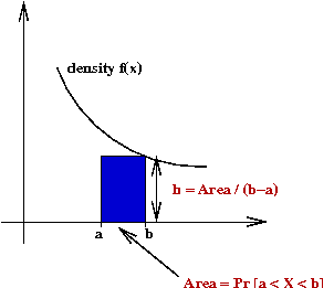
- But because \(F(b) - F(a) = \prob{a \leq X \leq b}\),
$$
\prob{a \leq X \leq b} \eql \int_a^b f(x)dx
$$
- As a corollary,
$$\eqb{
F(y) \eqt \prob{X \leq y} \\
\eqt \prob{-\infty \lt X \leq y} \\
\eqt \int_{-\infty}^y f(x) dx
}$$
- Finally,
\(F' = f\)
(Second fundamental theorem of calculus).
Exercise 35:
Find a description and picture of the standard Gaussian pdf.
What is the maximum value (height) of the pdf? Use a calculator
or write a program to compute this value as a decimal.
7.8 Histograms, pmfs and pdfs
What is the connection?
- We are used to the intuitive idea of a histogram,
which shows the spread of frequency-of-occurence.
- We sense that pmfs and pdfs show something similar
\(\Rightarrow\) This is more or less true, with some modifications.
Types of histograms:
- Let's start with the most basic histogram:
Suppose we are given 7 data: 1.6, 0.7, 2.4, 0.3, 1.8, 1.7, 0.4
- Step 1: find an appropriate range
\(\Rightarrow\) We'll use \([0, 2.5]\).
- Step 2: decide the granularity (number of bins)
\(\Rightarrow\) We'll use 5 bins.
- Step 3: Identify, for each bin, how many data values
fall into that bin.

- Note: the height of each bin is the number
of data falling into each bin.
- An alternative type of histogram is a relative
or proportional histogram:
- Here, we compute the proportion of data in each bin:

Exercise 36:
Consider the 3-coin flip example (with \(\probm{Heads]=0.6}\)).
Use a bin width of 1.0
and build a proportional histogram when the data is \(3, 1, 1, 0, 2, 0, 1, 2, 2, 2\).
Let's write some code for the 3-coin flip example:
- First, observe that the data is integers.
We will build bins to differentiate each possible outcome

- The program:
(source file)
	double numTrials = 100000;

	Coin coin = new Coin (0.6);

        // Build intervals to surround the values of interest.
        PropHistogram hist = new PropHistogram (-0.5, 3.5, 4);

	for (int t=0; t<numTrials; t++) {
            // #heads in 3 flips.
            int numHeads = coin.flip() + coin.flip() + coin.flip();
            hist.add (numHeads);
	}

        // View the histogram, text and graph.
        System.out.println (hist);
        hist.display ();
Exercise 37:
Run CoinExample5.java
to see what you get for a large number of samples.
You will also need Coin.java
and PropHistogram.java.
The relationship between the proportional histogram and pmf:
- Recall: pmf is for discrete rv's
\(\Rightarrow\) the list \(\prob{X=k}\) for each \(k\)
- We have selected each bin so that the height of bin \(k\)
is the proportion of times \(k\) occurs in the data.
- Clearly, in the limit,
Height of bin \(k \;\to\; \prob{X=k}\)
- Thus, the proportional histogram becomes the pmf in the limit.
Does this work for continuous rv's?
Exercise 38:
Use PropHistogram.java
and execute GaussianExample.java.
Does it work? Change the number of intervals from 10 to
20. What do you notice? Is the height correct?
Histograms for continuous rv's:
Exercise 39:
Modify computeHeights() in
PropHistogram.java
to compute heights as above for continuous rv's.
Then, execute GaussianExample.java.
Change the number of intervals from 10 to
20. Does it work?
Summary:
- In a regular histogram,
bin height = number of data in bin
- For discrete rv's, proportional histogram → pmf in the limit.
bin height = proportion of data in bin
- Another way of saying it: a proportional histogram
estimates the true pmf.
- For continuous rv's, density histogram → pmf in the limit.
bin height = proportion-of-data-in-bin / bin-width
- A density histogram estimates the true pdf.
Exercise 40:
Estimate the density of the time spent in the system
by a random customer in the QueueControl example.
To do this, you need to build a density histogram of
values of the variable
timeInSystem
in QueueControl.java.
7.9 Some well-known continuous rv's
Three important distributions (pdf shapes):
- Uniform:

- Exponential (γ = 4):

- Gaussian (also called Normal):
The Uniform distribution: if \(X\simm{Uniform}(a,b)\)
- \(a \lt b\) are two real numbers.
\(\Rightarrow\) Most common case: \(a=0, b=1\)
- \(X\) takes values in \([a,b]\) (\(a,b\) inclusive).
- \(X\) has pdf (defined, for generality, on the whole real line):
$$
f(x) \eql \left\{
\begin{array}{ll}
0 & \;\;\; x \lt a \\
\frac{1}{b-a} & \;\;\; a \leq x \leq b \\
0 & \;\;\; x \gt b \\
\end{array}
\right.
$$
- \(X\) has CDF
$$
F(x) \eql \left\{
\begin{array}{ll}
0 & \;\;\; x \lt a \\
\frac{x-a}{b-a} & \;\;\; a \leq x \leq b \\
1 & \;\;\; x \gt b \\
\end{array}
\right.
$$
- \(X\) has expected value
$$\eqb{
E[X] \eqt \int_{-\infty}^\infty f(x) dx \\
\eqt
\int_a^b \frac{1}{b-a} dx \\
\eqt
\frac{a+b}{2}
}$$
Exercise 41:
Suppose \(X\simm{Uniform}(a,b)\) and \([c,d]\) is a
sub-interval of \([a,b]\). Use either the pdf or
cdf to compute \(\prob{X\in [c,d]}\).
Exercise 42:
Suppose \(X\simm{Uniform}(0,1)\) and let
rv \(Y=1-X\). What is the distribution of \(Y\)?
- What is the range of \(Y\)?
- Use PropHistogram
to estimate the density (remember to scale by interval-width) of
\(Y\). Recall that RandTool.uniform() generates
values from the Uniform(0,1) distribution.
- How would you derive the pdf or CDF of \(Y\)?
The Exponential distribution: if \(X\simm{Exponential}(\gamma)\)
- The parameter \(\gamma\gt 0\) is a real number.
- \(X\) takes values in the positive half of the real-line.
- \(X\) has pdf (defined, for generality, on the whole real line):
$$
f(x) \eql
\left\{
\begin{array}{ll}
0 & \;\;\; x \leq 0\\
\gamma e^{-\gamma x} & \;\;\; x \gt 0
\end{array}
\right.
$$
- \(X\) has CDF
$$
F(x) \eql
\left\{
\begin{array}{ll}
0 & \;\;\; x \leq 0\\
1 - e^{-\gamma x} & \;\;\; x \gt 0
\end{array}
\right.
$$
- \(X\) has expected value
$$\eqb{
E[X] \eqt \int_{-\infty}^\infty f(x) dx \\
\eqt
\int_0^\infty \gamma e^{-\gamma x} dx \\
\eqt
\frac{1}{\gamma}
}$$
Exercise 43:
Suppose \(X\simm{Exponential}(\gamma)\).
- Write down an expression for \(\prob{X\gt a}\).
- Compute \(\prob{X\gt b+a \;|\; X\gt b}\).
Exercise 44:
Suppose \(X\simm{Exponential}(\gamma)\) with CDF \(F(x)\).
Write down an expression for \(F^{-1}(y)\), the inverse
of \(F\).
The Normal distribution: if \(X\simm{N}(\mu,\sigma^2)\)
- The parameter \(\mu\) is any real number.
- The parameter \(\sigma\) is any non-negative real number.
- \(X\) takes any real value.
- \(X\) has pdf
$$
f(x) \eql \frac{1}{\sqrt{2\pi} \sigma} e^{- \frac{(x-\mu)^2}{2\sigma^2}}
$$
- There is no closed-form CDF.
- \(X\) has expected value \(E[X] = \mu\).
7.10 Generating random values from distributions
We have used random values from various distributions,
but how does one write a program to generate them?
Key ideas:
- Since we are writing a (hopefully small) program,
the output cannot really be truly random.
\(\Rightarrow\) the goal is to make pseudo-random generators.
- Use the strange properties of numbers to make
a (pseudo-random) generator for Uniform(0,1) values.
- To generate values for some other distribution:
- Generate Uniform(0,1) values.
- Transform them so that the transformed values have
the desired distribution.
Note: Random-number generation is a topic of research by itself:
- Much work on high-quality Uniform(0,1) (or bit-stream)
generators.
- Similarly, there is much work on efficient transformations for
particular distributions.
Desirable properties for a pseudo-random generator:
- Should be repeatable:
\(\Rightarrow\) It should be possible to reproduce the sequence given some kind of initial "seed".
- Should be portable:
\(\Rightarrow\) It shouldn't be dependent on language, OS or hardware.
- Should be efficient:
\(\Rightarrow\) The calculations shouldn't take too long (simple
arithmetic, preferably).
- Should have some theoretical basis:
\(\Rightarrow\) Ideally, some number-theory results about its properties.
- (Contradiction) Should have good statistical properties:
\(\Rightarrow\) Should satisfy statistical tests for randomness.
Exercise 45:
What kinds of statistical tests? Is it enough that the
histogram resemble the \(U[0,1]\) pdf?
A simple algorithm: the Lehmer generator:
- For some large number \(M\), consider the set
\(S = {1,2,...,M-1}\).
- We will generate a number \(K\) in \(S\) and return \(U=\frac{K}{M}\).
\(\Rightarrow\) Output is between 0 and 1.
- If K is uniformly distributed between \(1\) and \(M-1\)
\(\Rightarrow\) \(U\) is approximately \(Uniform(0,1)\).
- Note: this means we'll never generate some values
like \((1+2)/2M\).
- Only remaining question: how do we pick uniformly among
the discrete elements in \(S={1,2,...,M-1}\)?
- Key idea:
- Consider two large numbers \(a\) and \(b\) (but both
\(a,b \lt M\)).
- Suppose we compute \(x = ab\) mod \(M\).
- Then \(x\) could be anywhere between \({1,2,...,M-1}\).
- Then, pick another two values for \(a\) and \(b\) and repeat.
- But how do we pick \(a\) and \(b\)?
The logic seems circular at this point.
- The key insight: use the previous value \(x\).
- Fix the values of \(a\) and \(b\).
- Compute \(x_1 = ab\) mod \(M\).
- Then, compute \(x_2 = ax_1\) mod \(M\).
- Then, compute \(x_3 = ax_2\) mod \(M\).
- ... etc
- We will call \(b = x_0\), the seed.
- It can be shown (number theory) that if \(M\) is prime,
the sequence of values \(x_1,x_2, ...,
x_p\) is periodic (and never repeats in between).
Furthermore, for some values of \(a\), \(p=M-1\).
- Example: \(M=2^{31}-1\) and \(a=48271\).
- Pseudocode:
     Algorithm: uniform ()
     // Assumes M and a are initialized.
     // Assumes x (global) has been initialized to seed value.
     1.   x = (a*x) mod M
     2.   return x
What about its properties?
- Some properties are obviously satisfied: portable, repeatable,
efficient (provided \(mod\) is efficient).
- The Lehmer generator has reasonably good statistical
properties for many applications.
- However, there are (stranger) generators with better
statistical properties.
Using a \(U[0,1]\) generator for discrete rv's:
- First, consider \(X\simm{Bernoulli}(0.6)\) as an example:

- Recall: \(X\) takes values 0 or 1 and \(\prob{X=1}=0.6\).
- Key idea: generate a uniform value \(U\).
- If \(0\lt U\lt 0.6\), return \(X=1\), else return \(X=0\).
- Pseudocode:
          Algorithm: generateBernoulli (p)
          Input: Bernoulli parameter p=Pr[success]
          1.   u = uniform ()
          2.   if u < p
          3.       return 1
          4.   else
          5.       return 0
          6.   endif
- This idea can be generalized: e.g., consider rv \(X\)
with pmf
\(\prob{X=0} = 0.064\)
\(\prob{X=1} = 0.288\)
\(\prob{X=2} = 0.432\)
\(\prob{X=3} = 0.216\)

Generate uniform value \(U\).
         if U < 0.064
             return 0
         else if U < 0.064 + 0.288
             return 1
         else if U < 0.064 + 0.288 + 0.432
             return 2
         else // if U < 1
             return 3
Exercise 46:
Add code to DiscreteGenExample.java
to implement the above generator, and to test it by building a histogram.
Let's generalize this to any discrete pmf of the type \(\prob{X=k} = ...\).
- We'll use the notation \(p_k = \prob{X=k}\).
- Define \(Q_k = \sum_{i\leq k} \prob{X=i}\)
- Then, the algorithm is:
Given uniform value \(U\), return the smallest
\(k\) such that \(U \gt Q_k\).
- Pseudocode:
    Algorithm: generateFromDiscretePmf ()
    // Assumes Q[k] have been computed.
    1.   u = uniform ()
    2.   k = 0
    3.   while Q[k] < u
    4.       k = k + 1
    5.   endwhile
    6.   return k
- This presents a problem when \(X\simm{Geometric}(p)\).
Here, \(X \in \{1,2,...\}\)
\(\Rightarrow\) Cannot pre-compute \(Q_k\)'s.
- Alternatively, we can compute the \(Q_k\)'s "as we go":
    Algorithm: generateFromDiscretePmf ()
    1.   u = uniform ()
    2.   k = 0
    3.   Q = Pr[X=0]
    4.   while Q < u
    5.       k = k + 1
    6.       Q = Q + Pr[X=k]
    7.   endwhile
    8.   return k
Exercise 47:
Add code to GeometricGenerator.java
to implement the above generator. The test code is already written.
Let's return to the 3-coin-flip example for a key insight:
- Recall the pmf:
\(\prob{X=0} = 0.064\)
\(\prob{X=1} = 0.288\)
\(\prob{X=2} = 0.432\)
\(\prob{X=3} = 0.216\)
- From which we can infer the CDF:
\(\prob{X \leq 0} = 0.064\)
\(\prob{X \leq 1} = 0.352 \) (= 0.064 + 0.288)
\(\prob{X\leq 2} = 0.784\) (= 0.064 + 0.288 + 0.432)
\(\prob{X\leq 3} = 1.000\) (= 0.064 + 0.288 + 0.432 + 0.216)
- Let's plot the CDF:

- Recall our generation algorithm:
Given uniform value \(u\), return the smallest \(k\)
such that \(U \gt Q_k\).

- Thus, it looks like we are using the CDF "in reverse".
We will use this idea for continuous rv's.
Using the inverse-CDF for continuous rv's:
- Suppose \(X\) is a continuous rv with CDF \(F(x)\).
- Suppose, further, that the inverse \(F^{-1}(y)\)
can be computed.
- Consider \(F^{-1}(U)\) where \(U\) is a uniform value.
- When \(U\) is a rv, so is \(g(U)\) for any function \(g\).
\(\Rightarrow\) In particular, \(F^{-1}(U)\) is a rv.
- Let \(H(x)\) be the CDF of the rv \(F^{-1}(U)\).
\(\Rightarrow\) Thus, \(H(x) = \prob{F^{-1}(U) \leq x}\).
- Let's work this through a few steps:
\(H(x)\)
\(= \prob{F^{-1}(U) \leq x}\)
\(= \prob{U \leq F(x)}\)
\(= F(x)\)
\(\Rightarrow\) \(F^{-1}(U)\) has the same CDF as \(X\).
\(\Rightarrow\) \(F^{-1}(U)\) has the same distribution as \(X\).
- Thus, we can use \(F^{-1}(U)\) to produce random
values of \(X\):
\(\Rightarrow\) Given uniform value \(U\), return \(F^{-1}(U)\).
- Pseudocode:
          Algorithm: generateFromContinuousCDF ()
          // Assumes inverse CDF F-1 is available.
          1.   u = uniform ()
          2.   return F-1(u)
Exercise 48:
Add code to ExponentialGenerator.java
to implement the above idea. Use the inverse-CDF you computed
earlier. The test code is written to produce a histogram.
Use your modified version of
PropHistogram.java to make
a density histogram. Compare the result with the actual density
(using \(\gamma = 4\)). How do you know your code worked?
About random generation:
- The inverse-CDF idea does not work easily for distributions like
the Normal:
\(\Rightarrow\) One needs to numerically approximate some inverse-CDFs.
- There are a host of techniques for specific distributions.
\(\Rightarrow\) random generation is a specialty in itself (several books).
- For simple simulations, the straightforward generators will suffice.
- For very large simulations (large numbers of samples)
\(\Rightarrow\) You'd want to use a more industrial-strength generator.
- Example: the Mersenne-Twister algorithm for uniform values.
- Another issue: many simulations require generating multiple
streams of random values
\(\Rightarrow\) Need to be careful that you don't introduce correlations
through careless use of generators.
7.1 Summary
What have we learned in this module?
- Prior to this, we learned how to reason about events:
- Events, sample spaces, probability measure.
- Combining events (intersection, union).
- Conditional probability, Bayes' rule, total-probability.
- A random variable (rv) measures numeric output from an experiment.
(As opposed to the outcome "King of Spades")
- Why is this useful?
You can perform arithmetic and other types of calculations
with numeric output, e.g., expected value.
- Two types: discrete and continuous.
- Discrete rv's have pmfs. Continuous rv's have pdfs.
- Both have CDFs defined the same way: \(F(y) = \prob{X \leq y}\).
- A proportional histogram becomes the pmf (in the limit).
- A density histogram becomes the pdf (in the limit).
(Minor technical issue: there are two limits here - the
number of samples, the size of the interval).
- The important discrete distributions: Bernoulli,
Discrete-Uniform, Binomial, Geometric, Poisson.
- The important continuous ones: Uniform, Exponential, Normal.
- The expected value is a calculation
performed on a pmf or pdf.
- For discrete rv's:
$$
E[X] \eql \sum_{k\in A} k \; \prob{X=k}
$$
- For continuous rv's:
$$
E[X]
\eql
\int_{-\infty}^\infty x f(x) dx
$$
© 2008, Rahul Simha