Module objectives
The main goals of this module:
- Describe commonly used gates, the key building blocks of circuits.
- Learn how the gates operate and are depicted in circuit diagrams.
- Explore the notion of universality: a small set of gates that
in combination can perform the same function as other gates.
6.1
Why circuits?
First, let's get a high-level view of what a quantum
computation looks like:
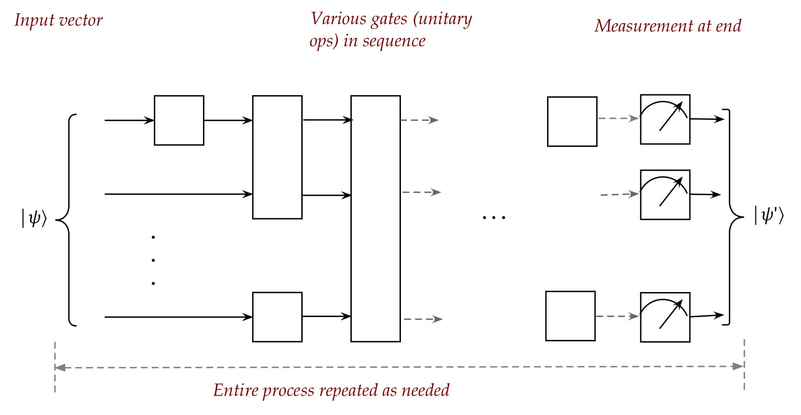
- The input vector is often \(\kt{00\ldots 0}\).
- Quite frequently, the input vector is converted to
$$
\ksi \eql \smf{1}{\sqrt{2^n}}
\parenl{ \kt{00\ldots 0} + \kt{00\ldots 1}
\ldots + \kt{11\ldots 1} }
$$
the equal-superposition vector.
- This vector is then fed into a sequence of unitary
operations (gates):
- The gates can be of various sizes.
- Each gate has the same number of outputs as inputs
(It has to, else it won't be unitary.)
- A qubit that skips a gate is equivalently transformed by the \(I\)
(identity) gate.
- Measurement occurs at the end, resulting in a probabilistic outcome.
- The whole sequence is repeated often, and statistical
analysis is performed on the collection of (probabilistic) outcomes.
- This is how a quantum algorithm works in the
standard circuit model.
Let's compare this with classical computing:
- First, compare with a simple calculator
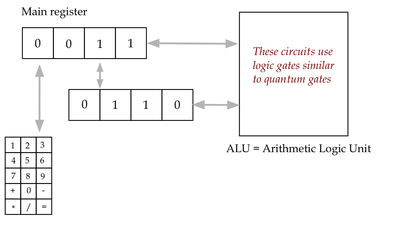
- Here too, a set of binary values flows through a circuit.
- The circuit is itself a collection of (Boolean) gates.
- Now with something more capable (a 1950's computer):
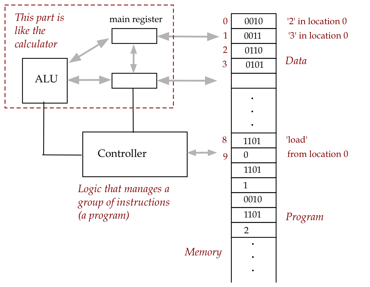
- This is now a whole level of additional power and complexity.
- One can write programs that execute in the same hardware
that "calculates".
- The programs themselves can be long and feature loops,
conditionals (if-then's) and other features.
- Within 20+ years after the earliest machines, the earliest
abstractions of algorithms began to appear, for example:
  Method: quickSort (data, L, R)
  Input: data - an array of size n with a subrange specified by L and R
  1.   if L ≥ R
  2.       return
  3.   endif

       // Partition the array and position partition element correctly.
  4.   p = partition (data, L, R)

  5.   quickSortRecursive (data, L, p-1)    // Sort left side
  6.   quickSortRecursive (data, p+1, R)    // Sort right side
- The astonishing power of such abstraction has led to the
modern world of computing.
- Many of these high-level abstractions (like recursion) are
hard to understand from the "circuit level view".
The contrast:
- Currently, quantum computing is in the 1940's era
of classical computing:
\(\rhd\)
The focus is on getting circuits to work at scale
- It's not even clear that the standard circuit model will dominate:
- Other proposed architectures apply measurements along the way.
- Yet others use mostly measurements.
- And more exotic approaches feature continuous,
as opposed to discrete, optimization.
- At a later time, one anticipates some integration into
classical hardware:
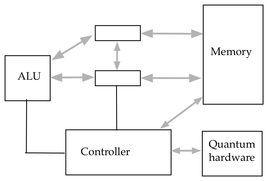
- What one hopes for the future (your generation):
\(\rhd\)
Powerful high-level abstractions akin to classical programming
- Questions that need answers:
- Which circuit model is best?
- What high-level abstractions are useful?
- How do these abstractions integrate classical and quantum?
- How can the circuit part be automated?
- What problems and algorithms are demonstrably (and
practically) faster on quantum hardware?
- What new and unexpected uses might arise from quantum computing?
The next steps for us:
- Learn about commonly used gates (this module)
- Learn to use the drawing conventions, Dirac and matrix representations
- Systematically build larger circuits (next module)
6.2
Commonly used 1-qubit gates: the Pauli gates
Let's begin with the four Pauli gates:
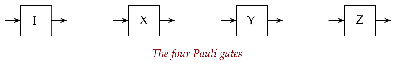
- In matrix and Dirac form:
$$\eqb{
I & \eql & \otr{0}{0} + \otr{1}{1} & \eql & \mat{1 & 0\\0 & 1} \\
X & \eql & \otr{0}{1} + \otr{1}{0} & \eql & \mat{0 & 1\\1 & 0} \\
Y & \eql & -i\otr{0}{1} + i\otr{1}{0} & \eql & \mat{0 & -i\\i & 0} \\
Z & \eql & \otr{0}{0} - \otr{1}{1} & \eql & \mat{1 & 0\\0 & -1} \\
}$$
- The action of \(X\) on a general qubit:
$$
X \parenl{ \alpha\kt{0} + \beta\kt{1} }
\eql
\parenl{ \otr{0}{1} + \otr{1}{0} }
\parenl{ \alpha\kt{0} + \beta\kt{1} }
\eql
\beta\kt{0} + \alpha\kt{1}
$$
Note:
- \(X\) switches the standard basis vectors:
$$\eqb{
X \kt{0} & \eql & \kt{1} \\
X \kt{1} & \eql & \kt{0} \\
}$$
- But not the Hadamard basis vectors:
$$\eqb{
X \kt{+} & \eql & \kt{+} \\
X \kt{-} & \eql & -\kt{-} \\
}$$
- Note:
$$
-\kt{-} \eql e^{i\pi}\kt{-}
$$
and so \(\kt{-}\) and \(-\kt{-}\) are the same qubit state
(global-phase equivalent).
- Next, consider \(Z\):
$$\eqb{
Z \parenl{ \alpha\kt{0} + \beta\kt{1} }
& \eql &
\parenl{ \otr{0}{0} - \otr{1}{1} }
\parenl{ \alpha\kt{0} + \beta\kt{1} } \\
& \eql &
\alpha\kt{0} - \beta\kt{1} \\
& \eql &
\alpha\kt{0} + e^{i\pi} \beta\kt{1}
}$$
which changes the sign of the \(\kt{1}\) component,
and therefore the relative phase of \(\alpha\kt{0} + \beta\kt{1}\).
- Some special cases for \(Z\):
$$\eqb{
Z\kt{0} & \eql & \kt{0} \\
Z\kt{1} & \eql & e^{i\pi} \kt{1} \\
Z\kt{+} & \eql & \kt{-} \\
Z\kt{-} & \eql & \kt{+} \\
}$$
Thus, \(Z\) switches the Hadamard vectors, but not \(\kt{0},\kt{1}\).
- Pauli gates are named in honor of Wolfgang Pauli, one of
the early major contributors to the development of quantum mechanics.
In-Class Exercise 1:
Use the Dirac form and
- Show that \(Y(\alpha\kt{0} + \beta\kt{1}) = i(\alpha\kt{1} - \beta\kt{0})\).
- Show that \(Y\) switches the Hadamard basis vectors.
(Remember global phase.)
Useful properties:
- Each Pauli gate is both unitary and Hermitian.
- The square of a Pauli gate is the identity:
$$
I^2 \eql X^2 \eql Y^2 \eql Z^2 \eql I
$$
- Pairwise identities:
$$\eqb{
XY & \eql & -YX & \eql & iZ \\
YZ & \eql & -ZY & \eql & iX \\
ZX & \eql & -XZ & \eql & iY \\
}$$
In-Class Exercise 2:
Prove the identity \(YZ = -ZY = iX\).
6.3
Commonly used 1-qubit gates: exponentiated-Pauli gates
It turns out that some exponentiated Pauli gates
like \(\sqrt{Z} = Z^{\frac{1}{2}}\) are unitary and useful.
Let's examine how to calculate the matrices:
- Recall this useful result (Module 4):
if \(A^2 = I\) then
$$
e^{i\theta A} \eql I \cos\theta + iA \sin\theta
$$
- Then, with \(A=X\)
$$\eqb{
e^{\frac{-i\theta}{2}X}
& \eql &
I\cos\sml{\frac{-\theta}{2}} + iX\sin\sml{\frac{-\theta}{2}} \\
& \eql &
\cos\sml{\frac{\theta}{2}} \mat{1 & 0\\ 0 & 1}
- \sin\sml{\frac{\theta}{2}} \mat{0 & i\\ i & 0} \\
& \eql &
\mat{ \cos\frac{\theta}{2} & -i \sin\frac{\theta}{2}\\
-i\sin\frac{\theta}{2} & \cos\frac{\theta}{2}}
}$$
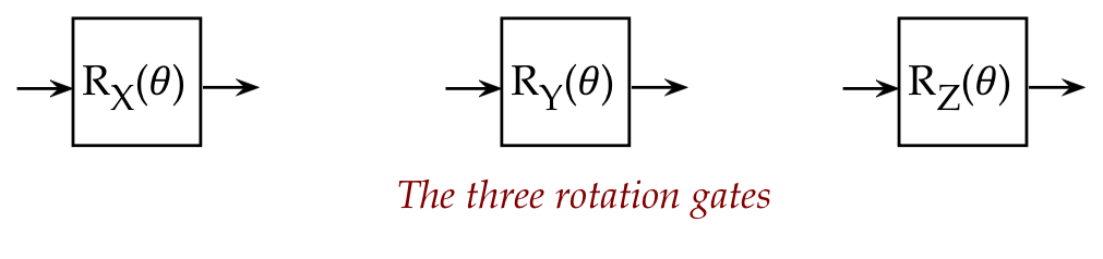
- This is given the special name \(R_X(\theta)\).
- One can similarly exponentiate \(Y, Z\) with the
same half-angle. Let's write these down:
$$\eqb{
R_X(\theta) & \eql & e^{\frac{-i\theta}{2}X}
& \eql &
\mat{ \cos\frac{\theta}{2} & -i \sin\frac{\theta}{2}\\
-i\sin\frac{\theta}{2} & \cos\frac{\theta}{2}} \\
R_Y(\theta) & \eql & e^{\frac{-i\theta}{2}Y}
& \eql &
\mat{ \cos\frac{\theta}{2} & -\sin\frac{\theta}{2}\\
\sin\frac{\theta}{2} & \cos\frac{\theta}{2}} \\
R_Z(\theta) & \eql & e^{\frac{-i\theta}{2}Z}
& \eql &
\mat{ e^{\frac{-i\theta}{2}} & 0\\
0 & e^{\frac{i\theta}{2}} } \\
}$$
- You might be curious: why use the half-angle in the definition?
- There is a geometric object called
the Bloch sphere
that is sometimes used to visualize actions on a single qubit.
- This is an artificial geometry that does not correspond to
anything in the real world.
- It turns out that the matrices above correspond to
\(\theta\)-rotations of the axes of this sphere.
- This is why the three matrices are sometimes called
rotation matrices.
- They perform rotations in the fictional Bloch sphere world.
- The exponential notation makes it obvious that
$$\eqb{
R_X(\theta_1 + \theta_2) & \eql & R_X(\theta_1) R_X(\theta_2) \\
R_Y(\theta_1 + \theta_2) & \eql & R_Y(\theta_1) R_Y(\theta_2) \\
R_Z(\theta_1 + \theta_2) & \eql & R_Z(\theta_1) R_Z(\theta_2) \\
}$$
For example:
$$
R_X(\theta_1) R_X(\theta_2)
\eql
e^{\frac{-i\theta_1}{2}X} e^{\frac{-i\theta_2}{2}X}
\eql
e^{\frac{-i(\theta_1+\theta_2)}{2}X}
\eql
R_X(\theta_1 + \theta_2)
$$
- All three are unitary. For example:
$$\eqb{
R_X(\theta)^\dagger R_X(\theta)
& \eql &
\mat{ \cos\frac{\theta}{2} & i \sin\frac{\theta}{2}\\
i\sin\frac{\theta}{2} & \cos\frac{\theta}{2}}
\mat{ \cos\frac{\theta}{2} & -i \sin\frac{\theta}{2}\\
-i\sin\frac{\theta}{2} & \cos\frac{\theta}{2}} \\
& \eql &
\mat{ \cos^2\frac{\theta}{2} + \sin^2\frac{\theta}{2} & 0\\
0 & \cos^2\frac{\theta}{2} + \sin^2\frac{\theta}{2} } \\
& \eql & I
}$$
In-Class Exercise 3:
Derive the matrix for \(R_Z(\theta)\) and show that
it is unitary. Is it Hermitian?
Three special cases:
- Recall:
$$
R_Z(\theta) \eql e^{\frac{-i\theta}{2}Z}
\eql
\mat{ e^{\frac{-i\theta}{2}} & 0\\
0 & e^{\frac{i\theta}{2}} } \\
$$
- With \(\alpha = -\frac{\theta}{2}\), we can write
$$
e^{i\alpha Z}
\eql
\mat{ e^{i\alpha} & 0\\
0 & e^{-i\alpha} } \\
\; \defn \;
T(\alpha)
$$
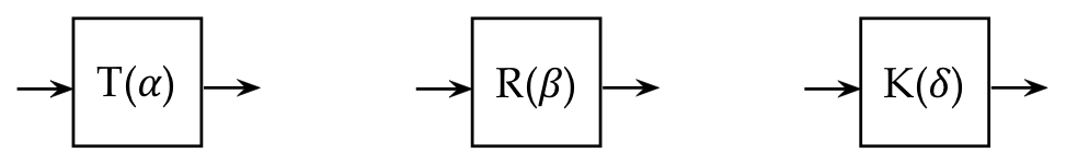
We'll call this the \(T(\alpha)\) gate, following the textbook.
- Consider a similar substitution \(\beta =
-\frac{\theta}{2}\) in
$$
R_Y(\theta)
\eql
e^{\frac{-i\theta}{2}Y}
\eql
\mat{ \cos\frac{\theta}{2} & -\sin\frac{\theta}{2}\\
\sin\frac{\theta}{2} & \cos\frac{\theta}{2}} \\
$$
This gives us
$$
e^{i\beta Y}
\eql
\mat{ \cos\beta & \sin\beta\\
-\sin\beta & \cos\beta} \\
\; \defn \;
R(\beta)
$$
It's slightly confusing but we'll call
this gate \(R(\beta)\) in keeping with the textbook.
- Finally, substitute \(A=I\) in
$$
e^{i\theta A} \eql I\cos\theta + iA \sin\theta
$$
to get
$$
e^{i\theta I} \eql I\cos\theta + iI \sin\theta
\eql e^{i\theta} I
$$
-
The gate
$$
K(\delta) \eql e^{i\delta} I
\eql
\mat{ e^{i\delta} & 0\\ 0 & e^{i\delta} }
$$
changes global-phase, which is occasionally useful in simplification.
- For example:
$$\eqb{
K(\delta) \parenl{ \alpha\kt{0} + \beta\kt{1} }
& \eql &
\mat{ e^{i\delta} & 0\\ 0 & e^{i\delta} }
\mat{\alpha \\ \beta}
& \eql &
e^{i\delta} \mat{\alpha \\ \beta}
& \eql &
e^{i\delta} \parenl{ \alpha\kt{0} + \beta\kt{1} }
}$$
- In summary:
$$\eqb{
T(\alpha)
& \eql &
\mat{ e^{i\alpha} & 0\\
0 & e^{-i\alpha} } \\
R(\beta)
& \eql &
\mat{ \cos\beta & \sin\beta\\
-\sin\beta & \cos\beta} \\
K(\delta)
& \eql &
\mat{ e^{i\delta} & 0\\ 0 & e^{i\delta} }
}$$
- Clearly, from the exponentiated origin,
$$\eqb{
T(\alpha_1 + \alpha_2)
& \eql & T(\alpha_1) T(\alpha_2) \\
R(\beta_1 + \beta_2)
& \eql & R(\beta_1) R(\beta_2) \\
K(\delta_1 + \delta_2)
& \eql & K(\delta_1) K(\delta_2) \\
}$$
- And
$$\eqb{
T(0) & \eql &
\mat{ e^{0} & 0\\
0 & e^{0} }
& \eql & I \\
R(0) & \eql &
\mat{ \cos 0 & \sin 0\\
-\sin 0 & \cos 0}
& \eql & I \\
}$$
- And, of course, all three are unitary. For example:
$$\eqb{
K(\delta)^\dagger K(\delta)
& \eql &
\parenl{ e^{i\delta} I }^\dagger \parenl{ e^{i\delta} I } \\
& \eql &
\parenl{ e^{i\delta}}^* I \; e^{i\delta} I \\
& \eql &
e^{-i\delta} I \; e^{i\delta} I \\
& \eql &
I
}$$
In-Class Exercise 4:
Show that the three operators \(T, R, K\) commute with
different parameters:
- \(T(\alpha_1)T(\alpha_2)=T(\alpha_2)T(\alpha_1)\)
- \(R(\beta_1)R(\beta_2)=R(\beta_2)R(\beta_1)\)
- \(K(\delta_1)K(\delta_2)=K(\delta_2)K(\delta_1)\)
6.4
Commonly used 1-qubit gates: powered Pauli gates
First, let's point out a consequence of global-phase equivalence:
- Recall what this means:
- Two vectors \(\ksi\) and \(\khi\) are
global-phase equivalent if
$$
\ksi \eql e^{i\theta} \khi
$$
for some \(\theta\).
- Both vectors then represent the same qubit state.
- Remember: measurement cannot tell them apart, because
the \(e^{i\theta}\) magnitude does not change probabilities.
- For example, in
$$
e^{i\theta}\alpha\kt{0} + e^{i\theta}\beta\kt{1}
$$
the probability for \(\kt{0}\) is
$$
\magsq{ e^{i\theta}\alpha }
\eql
\magsq{ e^{i\theta} } \magsq{ \alpha }
\eql
\magsq{ \alpha }
$$
- This means if
$$
\khi \eql U \ksi
$$
for any unitary \(U\) then
$$
e^{i\theta} \khi \eql (e^{i\theta} U) \ksi
$$
That is, \(U\) and \(e^{i\theta} U\) result in
two global-phase equivalent vectors.
- And so, one can drop or factor out \(e^{i\theta}\)
from any unitary \(e^{i\theta} U\).
Now let's turn to fractional powers of the Pauli operators.
The special property \(Z^2=I\) makes it possible
to easily derive \(Z^{\frac{1}{2}}\) and \(Z^{\frac{1}{4}}\):
- First, observe that
$$
e^{-i\frac{\pi}{2}Z}
\eql
\mat{e^{-\frac{\pi}{2}} & 0\\
0 & e^{\frac{\pi}{2}} }
\eql
\mat{-i & 0\\ 0 & i}
\eql
-iZ
$$
- Next because \(I^2 = I\), the \(A^2 = I\) exponentiation
property gives us
$$
e^{i\theta I} \eql I\cos\theta + iI\sin\theta
$$
and so
$$
e^{i\frac{\pi}{2} I} \eql iI
$$
- Combining the two results:
$$
e^{-iZ\frac{\pi}{2}} e^{iI\frac{\pi}{2}}
\eql
(-iZ) (iI)
\eql
Z
$$
- Now raise both sides to the power \(t\):
$$
Z^t \eql
e^{-iZt\frac{\pi}{2}} e^{iIt\frac{\pi}{2}}
$$
Thus, we have a way to compute fractional powers like
\(Z^{\frac{1}{2}}\) and \(Z^{\frac{1}{4}}\).
- A further simplification ensues from
$$\eqb{
e^{iIt\frac{\pi}{2}}
& \eql &
\left(e^{iI\frac{\pi}{2}}\right)^t \\
& \eql &
(iI)^t \\
& \eql &
\left( e^{i\frac{\pi}{2}} I \right)^t \\
& \eql &
\left( e^{i\frac{\pi}{2}} \right)^t I^t \\
& \eql &
e^{it\frac{\pi}{2}} I \\
}$$
- Then,
$$\eqb{
Z^t
& \eql &
e^{-iZt\frac{\pi}{2}} e^{iIt\frac{\pi}{2}} \\
& \eql &
R_Z(\pi t) e^{it\frac{\pi}{2}} I \\
& \eql &
e^{it\frac{\pi}{2}} R_Z(\pi t) I \\
& \eql &
e^{it\frac{\pi}{2}} R_Z(\pi t) \\
}$$
- With \(t=\frac{1}{2}\)
$$\eqb{
Z^{\frac{1}{2}}
& \eql &
e^{i\frac{\pi}{4}} R_Z(\frac{\pi}{2}) \\
& \eql &
e^{i\frac{\pi}{4}}
\mat{ e^{-i\frac{\pi}{4}} & 0\\
0 & e^{i\frac{\pi}{4}} } \\
& \eql &
\mat{ 1 & 0 \\
0 & e^{i\frac{\pi}{2}} } \\
& \eql &
\mat{ 1 & 0 \\
0 & i} \\
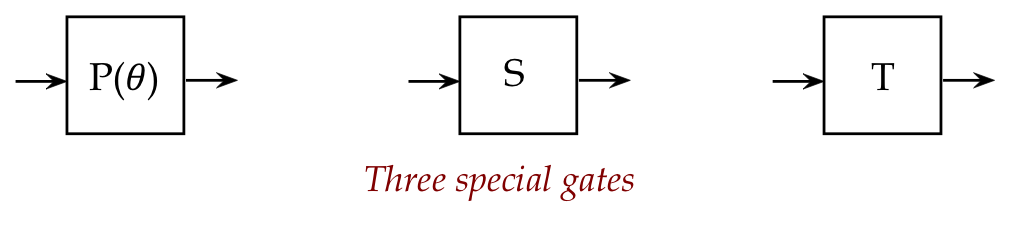
& \; \defn \; &
\mbox{S-gate}
}$$
- Similarly, with \(t=\frac{1}{4}\), we get
$$\eqb{
Z^{\frac{1}{4}}
& \eql &
\mat{ 1 & 0 \\
0 & e^{i\frac{\pi}{4}} } \\
& \; \defn \; &
\mbox{T-gate}
}$$
- For general \(t=\theta\),
$$\eqb{
Z^\theta
& \eql &
e^{i\theta\frac{\pi}{2}} R_Z(\pi \theta) \\
& \eql &
e^{i\theta\frac{\pi}{2}}
\mat{ e^{- i\theta\frac{\pi}{2}} & 0 \\
0 & e^{i\theta\frac{\pi}{2}} } \\
& \eql &
\mat{ 1 & 0 \\
0 & e^{i\pi\theta} } \\
}$$
- When substituting \(t = \frac{\theta}{\pi}\):
$$\eqb{
Z^{ \frac{\theta}{\pi} }
& \eql &
\mat{ 1 & 0 \\
0 & e^{i\theta} } \\
& \; \defn \; &
\mbox{\(P(\theta)\)-gate}
}$$
This achieves a change in relative phase in a qubit:
$$
P(\theta) \parenl{ \alpha\kt{0} + \beta\kt{1} }
\eql
\mat{ 1 & 0 \\
0 & e^{i\theta} }
\mat{\alpha \\ \beta}
\eql
\mat{\alpha \\ e^{i\theta}\beta}
\eql
\alpha\kt{0} + e^{i\theta} \beta\kt{1}
$$
- Note: the vectors
$$
\alpha\kt{0} + \beta\kt{1}
$$
and
$$
\alpha\kt{0} + e^{i\pi\theta} \beta\kt{1}
$$
do not represent the same qubit state.
- To summarize:
$$\eqb{
P(\theta) & \eql &
\mat{ 1 & 0 \\
0 & e^{i\theta} } & & \\
S & \eql &
\mat{ 1 & 0 \\
0 & i} & \eql & P(\smf{\pi}{2}) \\
T & \eql &
\mat{ 1 & 0 \\
0 & e^{i\frac{\pi}{4}} } & \eql & P(\smf{\pi}{4}) \\
}$$
- All are unitary. For example:
$$
S^\dagger S
\eql
\mat{ 1 & 0 \\ 0 & -i}
\mat{ 1 & 0 \\ 0 & i}
\eql I
$$
- Note: the \(P(\theta)\) gate will play a significant role in
the implementation of Shor's algorithm.
In-Class Exercise 5:
Show that \(P(\theta)\) is unitary.
In-Class Exercise 6:
Show that the same property that we derived for \(Z\)
can be derived for \(X\), that is,
\(e^{-i\frac{\pi}{2}X} = -iX\).
This means fractional powers of \(X\) can be computed
in the same way, as shown in one of the solved examples.
Finally, let's list the important powers for convenience:
$$\eqb{
X^{\frac{1}{2}} & \eql &
\frac{1}{2} \mat{1+i & 1-i\\ 1-i & 1+i}
& \mbx{This is one of many \(\sqrt{X}\)} \\
Y^{\frac{1}{2}} & \eql &
\isqt{e^{i\frac{\pi}{4}}} \mat{1 & -1\\ 1 & 1}
& \mbx{Useful in constructing \(H\)} \\
Z^{\frac{1}{2}} & \eql &
\mat{1 & 0\\ 0 & i}
& \mbx{S-gate} \\
Z^{\frac{1}{4}} & \eql &
\mat{1 & 0\\ 0 & e^{i\frac{\pi}{4}} }
& \mbx{T-gate} \\
Z^{\frac{\theta}{\pi}} & \eql &
\mat{1 & 0\\ 0 & e^{i\theta} }
& \mbx{\(P(\theta)\)-gate} \\
}$$
6.5
Commonly used 1-qubit gates: Hadamard
We have already introduced the Hadamard, but let's include it
here for completeness, and also add some new properties:
- The Hadamard gate is
$$
H \eql \mat{\isqt{1} & \isqt{1}\\ \isqt{1} & -\isqt{1} }
\eql \isqts{1} \mat{1 & 1\\ 1 & -1}
$$
- It converts back and forth between standard and H-basis vectors:
$$\eqb{
H \kt{0} & \eql & \kt{+} \\
H \kt{1} & \eql & \kt{-} \\
H \kt{+} & \eql & \kt{0} \\
H \kt{-} & \eql & \kt{1} \\
}$$
- And we've seen its fundamental role in creating n-qubit superpositions:
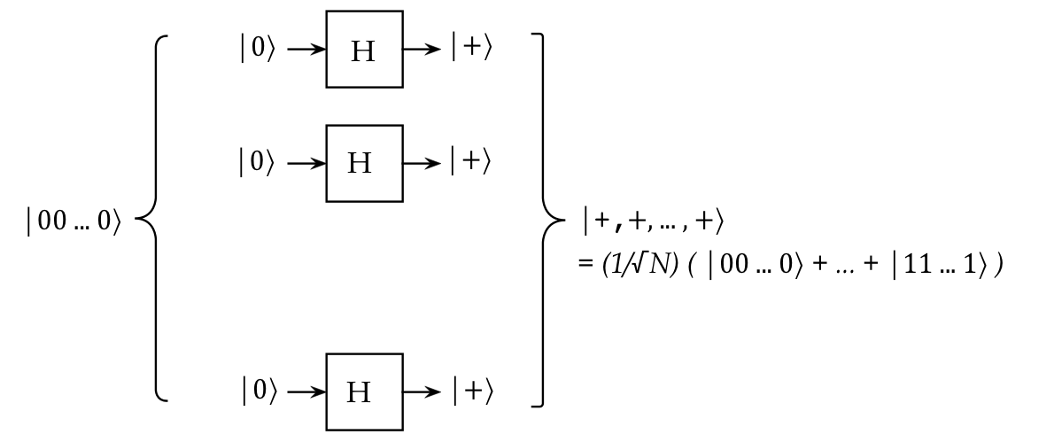
Here, for the n-qubit case:
$$\eqb{
& & \hspace{-20pt}
(H \otimes H \otimes \ldots \otimes H)
\kt{00\ldots 0} & \mbx{Apply \(H\) to each qubit} \\
& \eql &
\smf{1}{\sqrt{N}} \parenl{ \kt{00\ldots 0} + \kt{00\ldots 1} + \ldots + \kt{11\ldots 1} }
& \mbx{Algebra shows that it produces this equal superposition}\\
}$$
- Observe:
- We've performed \(n\) operations above (a polynomial number),
in parallel.
- And obtained an exponential number of vectors in
the superposition: \(N=2^n\).
- We often use the decimal version of the standard
basis
$$\eqb{
\kt{0} & \eql & \kt{00\ldots 0} \\
\kt{1} & \eql & \kt{00\ldots 1} \\
\kt{2} & \eql & \kt{0\ldots 10} \\
\kt{3} & \eql & \kt{0\ldots 11} \\
& \vdots & \\
\kt{N-1} & \eql & \kt{1\ldots 11} \\
}$$
where \(N = 2^n\).
- Let's rewrite the \(n\)-tensored Hadamard acting on
all-\(\kt{0}\) as:
$$\eqb{
& & \hspace{-20pt}
(H \otimes H \otimes \ldots \otimes H)
\kt{00\ldots 0} \\
& \eql &
\smf{1}{\sqrt{N}} \parenl{ \kt{00\ldots 0} + \kt{00\ldots 1} + \ldots + \kt{11\ldots 1} } \\
& \eql &
\smf{1}{\sqrt{N}} \parenl{ \kt{0} + \kt{1} + \ldots + \kt{N-1} } \\
& \eql &
\smf{1}{\sqrt{N}} \sum_{k=0}^{N-1} \kt{k}\\
}$$
The Hadamard with other 1-qubit gates:
- The following identities are easily established:
$$\eqb{
H \, X \, H & \eql & Z \\
H \, Z \, H & \eql & X \\
H \, Y \, H & \eql & -Y \\
H \, R_X(\theta) \, H & \eql & R_Z(\theta) \\
H \, R_Z(\theta) \, H & \eql & R_X(\theta) \\
H \, R_Y(\theta) \, H & \eql & R_Y(-\theta) \\
}$$
- For example:
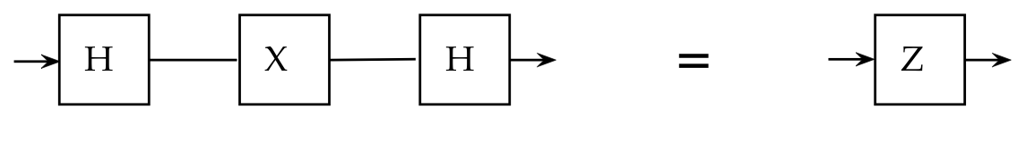
$$\eqb{
H \, X \, H
& \eql &
\isqts{1} \mat{1 & 1\\ 1 & -1}
\mat{0 & 1\\ 1 & 0}
\isqts{1} \mat{1 & 1\\ 1 & -1} \\
& \eql &
\smf{1}{2}
\mat{1 & 1\\ 1 & -1}
\mat{1 & -1\\ 1 & 1} \\
& \eql &
\smf{1}{2}
\mat{2 & 0\\ 0 & -2} \\
& \eql &
Z
}$$
- Another example:
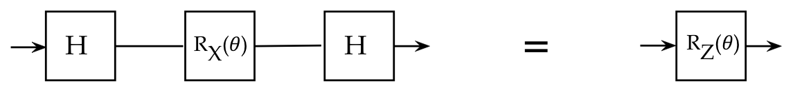
$$\eqb{
H \, R_X(\theta) \, H
& \eql &
\isqts{1} \mat{1 & 1\\ 1 & -1}
\mat{ \cos\frac{\theta}{2} & -i \sin\frac{\theta}{2}\\
-i\sin\frac{\theta}{2} & \cos\frac{\theta}{2}}
\isqts{1} \mat{1 & 1\\ 1 & -1} \\
& \eql &
\smf{1}{2} \mat{1 & 1\\ 1 & -1}
\mat{ e^{-i\frac{\theta}{2}} & e^{i\frac{\theta}{2}} \\
e^{-i\frac{\theta}{2}} & -e^{i\frac{\theta}{2}} } \\
& \eql &
\smf{1}{2}
\mat{ 2e^{-i\frac{\theta}{2}} & 0\\
0 & -2e^{i\frac{\theta}{2}} } \\
& \eql &
R_Z(\theta)
}$$
In-Class Exercise 7:
Show the two \(Y\) properties:
- \(H \, Y \, H = -Y\)
- \(H \, R_Y(\theta) \, H = R_Y(-\theta)\)
6.6
Summary of important 1-qubit gates
For convenience, let's list all the gates so far.
The main Pauli gates:
$$\eqb{
I & \eql & \mat{1 & 0\\0 & 1} \\
X & \eql & \mat{0 & 1\\1 & 0} \\
Y & \eql & \mat{0 & -i\\i & 0} \\
Z & \eql & \mat{1 & 0\\0 & -1} \\
}$$
The three rotation gates \(R_X(\theta), R_Y(\theta),
R_Z(\theta)\):
$$\eqb{
R_X(\theta) & \eql & e^{\frac{-i\theta}{2}X}
& \eql &
\mat{ \cos\frac{\theta}{2} & -i \sin\frac{\theta}{2}\\
-i\sin\frac{\theta}{2} & \cos\frac{\theta}{2}} \\
R_Y(\theta) & \eql & e^{\frac{-i\theta}{2}Y}
& \eql &
\mat{ \cos\frac{\theta}{2} & -\sin\frac{\theta}{2}\\
\sin\frac{\theta}{2} & \cos\frac{\theta}{2}} \\
R_Z(\theta) & \eql & e^{\frac{-i\theta}{2}Z}
& \eql &
\mat{ e^{\frac{-i\theta}{2}} & 0\\
0 & e^{\frac{i\theta}{2}} } \\
}$$
The \(T(\alpha),R(\beta)\) and \(K(\delta)\) gates:
$$\eqb{
T(\alpha)
& \eql &
e^{i\alpha Z}
& \eql &
\mat{ e^{i\alpha} & 0\\
0 & e^{-i\alpha} } \\
R(\beta)
& \eql &
e^{i\beta Y}
& \eql &
\mat{ \cos\beta & \sin\beta\\
-\sin\beta & \cos\beta} \\
K(\delta)
& \eql &
e^{i\delta I}
& \eql &
\mat{ e^{i\delta} & 0\\ 0 & e^{i\delta} }
}$$
The special gates \(P(\theta), S\) and \(T\):
$$\eqb{
P(\theta) & \eql & Z^{\frac{\theta}{\pi}}
& \eql &
\mat{ 1 & 0 \\
0 & e^{i\theta} } \\
S & \eql & Z^{\frac{1}{2}}
& \eql &
\mat{ 1 & 0 \\
0 & i} \\
T & \eql & Z^{\frac{1}{4}}
& \eql &
\mat{ 1 & 0 \\
0 & e^{i\frac{\pi}{4}} } \\
}$$
And of course the Hadamard:
$$
H \eql \mat{\isqt{1} & \isqt{1}\\ \isqt{1} & -\isqt{1} }
\eql \isqt{1} \mat{1 & 1\\ 1 & -1}
$$
In-Class Exercise 8:
- Compute \(R_Z(\frac{\pi}{2}) R_X(\frac{\pi}{2}) R_Z(\frac{\pi}{2}) \)
- Then show that
\(H = K(\frac{\pi}{2}) R_Z(\frac{\pi}{2}) R_X(\frac{\pi}{2}) R_Z(\frac{\pi}{2}) \)
6.7
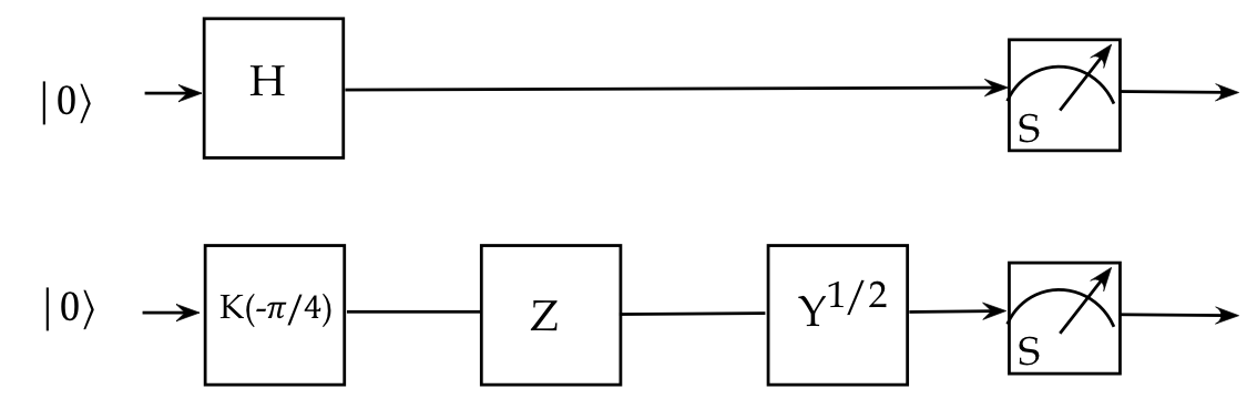
An example with 1-qubit gates
Let's analyze an example circuit in a few different ways:
where
$$
Y^{\frac{1}{2}} \eql
\isqt{e^{i\frac{\pi}{4}}} \mat{1 & -1\\ 1 & 1}
$$
- First, let's infer the stages and implied tensored operators:
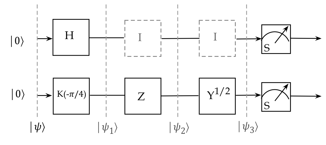
- We see that the input state is
\(\ksi \eql \kt{00}\)
- The first 2-qubit unitary is: \(H \otimes K(-\frac{\pi}{4})\),
resulting in state \(\kt{\psi_1}\):
$$
\kt{\psi_1} \eql \parenl{ H \otimes K(\smm{-\frac{\pi}{4}}) } \ksi
$$
- After this, the 2-qubit unitary \(I\otimes Z\) acts on
\(\kt{\psi_1}\):
$$
\kt{\psi_2} \eql \parenl{I \otimes Z} \kt{\psi_1}
$$
- Finally,
$$
\kt{\psi_3} \eql \parenl{I \otimes Y^{\frac{1}{2}} } \kt{\psi_2}
$$
- Let's now build the three tensored operators.
- The first one is
$$\eqb{
H \otimes K(\smm{-\frac{\pi}{4}})
& \eql &
\isqt{1} \mat{1 & 1\\ 1 & -1}
\; \otimes \;
e^{-i\frac{\pi}{4}} \mat{1 & 0\\ 0 & 1}\\
& \eql &
\isqt{e^{-i\frac{\pi}{4}}}
\mat{1 & 1\\ 1 & -1}
\; \otimes \;
\mat{1 & 0\\ 0 & 1} \\
& \eql &
\isqt{e^{-i\frac{\pi}{4}}}
\mat{1 & 0 & 1 & 0\\
0 & 1 & 0 & 1\\
1 & 0 & -1 & 0\\
0 & 1 & 0 & -1}
}$$
- The second:
$$
I \otimes Z
\eql
\mat{1 & 0\\ 0 & 1}
\otimes
\mat{1 & 0\\ 0 & -1}
\eql
\mat{1 & 0 & 0 & 0\\
0 & -1 & 0 & 0\\
0 & 0 & 1 & 0\\
0 & 0 & 0 & -1}
$$
- And
$$
I \otimes Y^{\frac{1}{2}}
\eql
\isqt{e^{i\frac{\pi}{4}}}
\mat{1 & -1 & 0 & 0\\
1 & 1 & 0 & 0\\
0 & 0 & 1 & -1\\
0 & 0 & 1 & 1}
$$
- At this stage, we could multiply into the vectors
to obtain \(\kt{\psi_1}, \kt{\psi_2}, \kt{\psi_3}\).
- However, we know that unitaries in sequence can be combined
simply by multiplication:
$$\eqb{
& \; & \parenl{ I \otimes Y^{\frac{1}{2}} }
\parenl{ I \otimes Z }
\parenl{ H \otimes K(\smm{-\frac{\pi}{4}}) } \\
& \; & \eql
\isqt{e^{-i\frac{\pi}{4}}}
\isqt{e^{i\frac{\pi}{4}}}
\mat{1 & -1 & 0 & 0\\
1 & 1 & 0 & 0\\
0 & 0 & 1 & -1\\
0 & 0 & 1 & 1}
\mat{1 & 0 & 0 & 0\\
0 & -1 & 0 & 0\\
0 & 0 & 1 & 0\\
0 & 0 & 0 & -1}
\mat{1 & 0 & 1 & 0\\
0 & 1 & 0 & 1\\
1 & 0 & -1 & 0\\
0 & 1 & 0 & -1} \\
& \; & \eql
\frac{1}{2}
\mat{1 & 1 & 1 & 1\\
1 & -1 & 1 & -1\\
1 & 1 & -1 & -1\\
1 & -1 & -1 & 1}
}$$
- While in general, one might have to use tools to compute
larger matrices, in this particular case, an algebraic solution
exists to confirm the above:
$$
\parenl{ I \otimes Y^{\frac{1}{2}} }
\parenl{ I \otimes Z }
\parenl{ H \otimes K(\smm{-\frac{\pi}{4}}) }
\eql
H \otimes Y^{\frac{1}{2}} \, Z \, K(\smm{-\frac{\pi}{4}})
\eql
H \otimes H
$$
The latter is
$$
\isqts{1} \mat{1 & 1\\ 1 & -1}
\otimes
\isqts{1} \mat{1 & 1\\ 1 & -1}
\eql
\frac{1}{2}
\mat{1 & 1 & 1 & 1\\
1 & -1 & 1 & -1\\
1 & 1 & -1 & -1\\
1 & -1 & -1 & 1}
$$
as expected.
In-Class Exercise 9:
- Verify that \(Y^{\frac{1}{2}}\, Z\, K(-\frac{\pi}{4}) = H\).
- Compute the three vectors
\(\kt{\psi_1}, \kt{\psi_2}, \kt{\psi_3}\)
at each step.
6.8
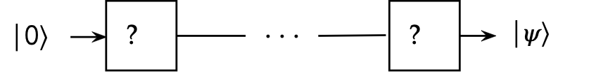
Setting a 1-qubit state
Suppose we want to set a qubit to an arbitrary value
\(\ksi = \alpha\kt{0} + \beta\kt{1}\).
Typically, we start with a well-known easy-for-hardware
state like \(\kt{0}\) and ask which unitary operations in sequence
could achieve the desired state:
Let's start with the simpler case where \(\alpha,\beta\) are real:
- Recall that
$$
R_Y(\theta) \eql e^{\frac{-i\theta}{2}Y}
\eql
\mat{ \cos\frac{\theta}{2} & -\sin\frac{\theta}{2}\\
\sin\frac{\theta}{2} & \cos\frac{\theta}{2}} \\
$$
- From this,
$$
R_Y(2\theta) \eql
\mat{ \cos\theta & -\sin\theta\\
\sin\theta & \cos\theta } \\
$$
and thus
$$\eqb{
R_Y(2\theta) \kt{0} & \eql &
\mat{ \cos\theta & -\sin\theta\\
\sin\theta & \cos\theta }
\mat{1\\ 0} \\
& \eql &
\cos\theta\kt{0} + \sin\theta\kt{1} \\
& \eql &
\cos\theta\kt{0} + \sqrt{1 - \cos^2 \theta} \kt{1}
}$$
- Since \(\alpha,\beta\) in \(\alpha\kt{0} + \beta\kt{1}\) are real we can equate
$$
\beta \eql \sqrt{1 - \alpha^2}
$$
and pick \(\theta\) so that
$$
\cos\theta \eql \alpha
$$
That is,
$$
\theta \eql \cos^{-1} \alpha
$$
- Then,
$$\eqb{
R_Y(2\cos^{-1}\alpha) \kt{0}
& \eql &
\cos(\cos^{-1}\alpha) \kt{0} \: + \:
\sqrt{1 - (\cos(\cos^{-1}\alpha))^2} \kt{1} \\
& \eql &
\alpha \kt{0} + \beta\kt{1}
}$$
Next, consider the case \(\alpha,\beta\) are complex:
- First, let's write \(\alpha,\beta\) in polar form:
$$\eqb{
\alpha & \eql & r_1 e^{i\theta_1} \\
\beta & \eql & r_2 e^{i\theta_2} \\
}$$
From which
$$\eqb{
\ksi & \eql & r_1 e^{i\theta_1} \kt{0} + r_2 e^{i\theta_2}\kt{1} \\
& \eql &
e^{i\theta_1} \parenl{r_1\kt{0} + r_2 e^{i\theta_2-\theta_1}\kt{1} }\\
& \equiv & r_1\kt{0} + r_2 e^{i\theta_2-\theta_1}\kt{1}
}$$
where we've used global phase equivalence in the last step.
- Since \(r_1,r_2\) are real and \(r_1^2+r_2^2=1\),
we can use the earlier idea
in producing \(r_1\kt{0} + r_2 \kt{1}\):
$$
R_Y(2\cos^{-1} r_1) \kt{0}
\eql r_1\kt{0} + r_2 \kt{1}
$$
- Next, recall the phase-gate
$$
P(\gamma) \eql \mat{1 & 0\\ 0 & e^{i\gamma}}
$$
and its action on a generic qubit state:
$$
P(\gamma) \parenl{a \kt{0} + b\kt{1}}
\eql
a \kt{0} + e^{i\gamma} b\kt{1}
$$
- Thus, to add a phase of \(\theta_2-\theta_1\):
$$
P(\theta_2-\theta_1) \parenl{ r_1\kt{0} + r_2 \kt{1} }
\eql
r_1\kt{0} + r_2 e^{i\theta_2-\theta_1}\kt{1}
$$
Which gives us the desired qubit state.
- To summarize:
$$
P(\theta_2-\theta_1) R_Y(2\cos^{-1} r_1) \kt{0}
\eql
r_1\kt{0} + r_2 e^{i\theta_2-\theta_1}\kt{1}
$$
6.9
Common 2-qubit gates
Every tensor of two 1-qubit unitaries is a 2-qubit unitary.
However, many 2-qubit unitaries cannot be written as such a
tensor.
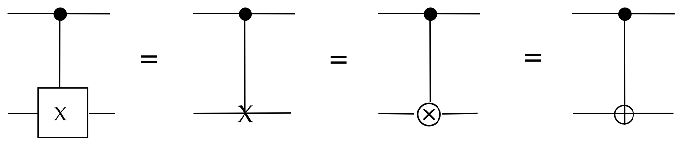
Let's start with the most important one: \(\cnot\)
- We have already seen \(\cnot\) but let's review briefly.
- These four circuit-diagram symbols are often used:
- In matrix form and Dirac forms:
$$\eqb{
\cnot & \eql &
\otr{0}{0} \otimes I \; + \; \otr{1}{1} \otimes X \\
& \eql &
\otr{00}{00} + \otr{01}{01} + \otr{10}{11} + \otr{11}{10} \\
& \eql &
\mat{1 & 0 & 0 & 0\\
0 & 1 & 0 & 0\\
0 & 0 & 0 & 1\\
0 & 0 & 1 & 0}
}$$
Thus, even though \(\cnot\) cannot be written as a direct tensor,
it is a sum of two tensors.
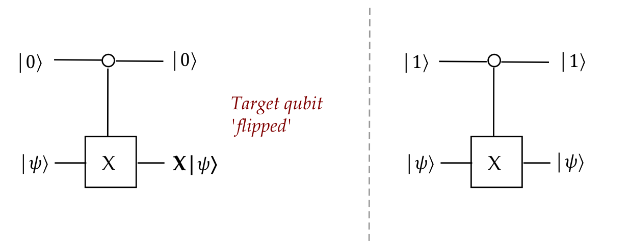
- The top bit is called the control bit
when the control bit is either \(\kt{0}\) or \(\kt{1}\).
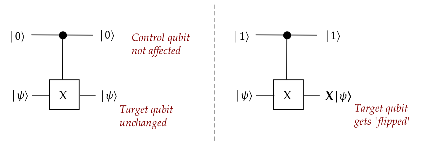
$$\eqb{
\parenl{ \otr{0}{0} \otimes I \; + \; \otr{1}{1} \otimes X }
\parenl{ \kt{0} \otimes \ksi }
& \eql & \kt{0} \otimes \ksi \\
\parenl{ \otr{0}{0} \otimes I \; + \; \otr{1}{1} \otimes X }
\parenl{ \kt{1} \otimes \ksi }
& \eql & \kt{1} \otimes X \ksi \\
}$$
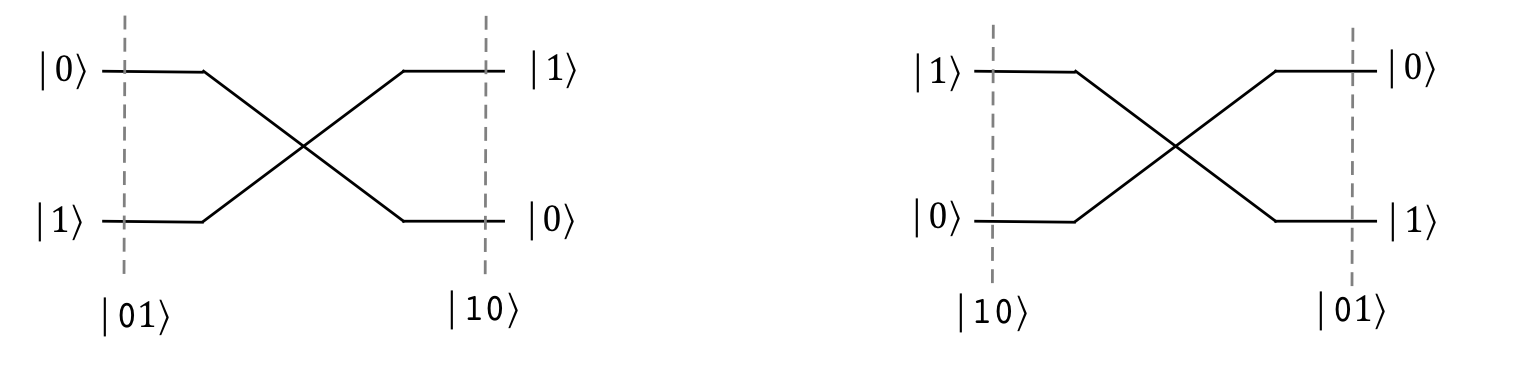
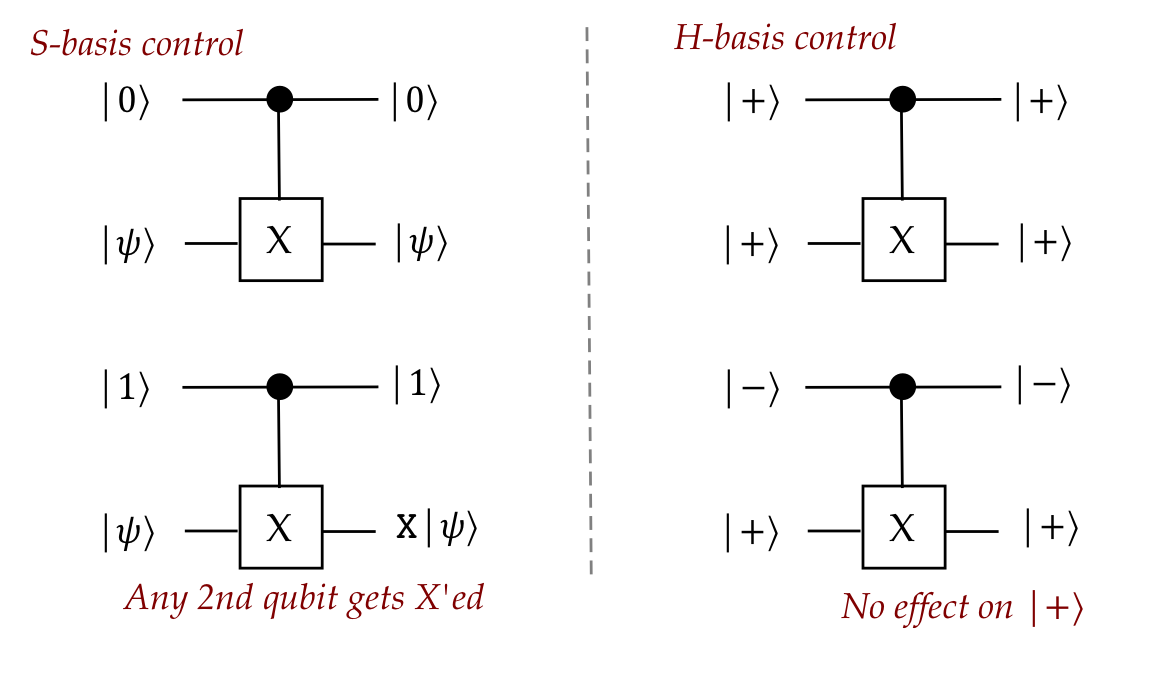
- On the standard basis vectors, \(\cnot\) produces
$$\eqb{
\cnot \kt{00} & \eql & \kt{00} \\
\cnot \kt{01} & \eql & \kt{01} \\
\cnot \kt{10} & \eql & \kt{11} \\
\cnot \kt{11} & \eql & \kt{10} \\
}$$
- This 'flipping' does not necessarily happen with other
vectors in the control bit:
$$\eqb{
\cnot \kt{+, +} & \eql & \kt{+,+} \\
\cnot \kt{-, +} & \eql & \kt{-,+}
}$$
In neither case does the second qubit change.
However, with \(\kt{+}, \kt{-1}\), the second qubit flips the first:
$$\eqb{
\cnot \kt{+, -} & \eql & \kt{-,-} \\
\cnot \kt{-, -} & \eql & \kt{+,-}
}$$
- Summary of properties:
- \(\cnot\) is Hermitian: \(\cnot = \cnot^\dagger\)
- \(\cnot\) is its own inverse
- \(\cnot\) can entangle or disentangle
$$\eqb{
\kt{\Phi^+} & \eql & \cnot \kt{+}\kt{0}
& \mbx{Create entangled Bell state} \\
\cnot \kt{\Phi^+} & \eql & \kt{+}\kt{0}
& \mbx{\(\cnot\) is its own inverse, disentangles Bell state} \\
}$$
- Recall:
$$
\kt{\Phi^+} \eql \isqts{1} \parenl{ \kt{00} + \kt{11} }
$$
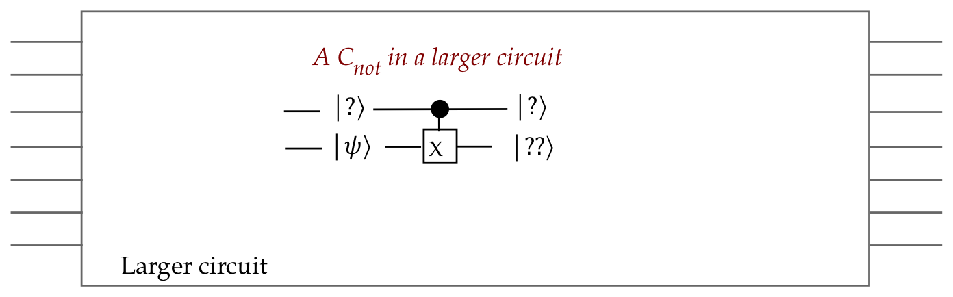
- Important:
- The term "control" makes sense only when standard-basis
vectors are the inputs.
- We will still use such gates with linear-combinations of
standard-basis vectors.
- In this case, additional reasoning will be needed to ensure
the results make sense.
\(\cnot\) variations:
- One can easily change the role of the control bit to flip when
it's \(\kt{0}\):
$$
\cnot^0 \eql \otr{0}{0} \otimes X \; + \; \otr{1}{1} \otimes I
\eql
\mat{0 & 1 & 0 & 0\\
1 & 0 & 0 & 0\\
0 & 0 & 1 & 0\\
0 & 0 & 0 & 1}
$$
- Or make \(\cnot\) "upside-down" by using the second qubit as control:
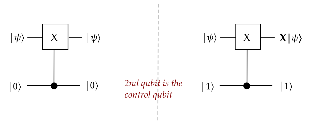
We'll call this \(\bar{C}_{\scriptsize NOT}\).
- It's easy to show that \(\bar{C}_{\scriptsize NOT}\)
can be implemented with \(\cnot\) and some Hadamards:
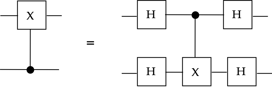
That is,
$$
\bar{C}_{\scriptsize NOT} \eql (H \otimes H) \cnot (H \otimes H)
$$
In-Class Exercise 10:
Write down the Dirac and matrix forms of the
two versions of the "upside-down", once with \(\kt{1}\)
achieving the flip, and once with \(\kt{0}\). Show using
Dirac notation that each is its own inverse.
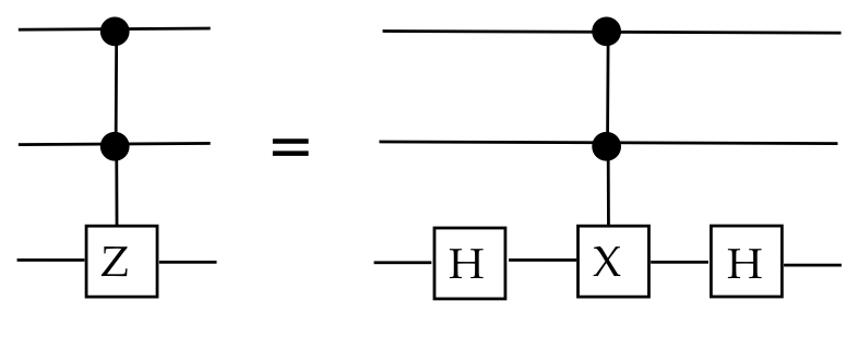
The \(\cz\) gate:
- \(\cz\) = Controlled-Z
- In Dirac and matrix forms:
$$\eqb{
\cz & \eql &
\otr{0}{0} \otimes I \; + \; \otr{1}{1} \otimes Z \\
& \eql &
\otr{00}{00} + \otr{01}{01} + \otr{10}{10} - \otr{11}{11} \\
& \eql &
\mat{1 & 0 & 0 & 0\\
0 & 1 & 0 & 0\\
0 & 0 & 1 & 0\\
0 & 0 & 0 & -1}
}$$
- Its action on the 2-qubit standard basis:
$$\eqb{
\cz \kt{00} & \eql & \kt{00} \\
\cz \kt{01} & \eql & \kt{01} \\
\cz \kt{10} & \eql & \kt{10} \\
\cz \kt{11} & \eql & -\kt{11} \\
}$$
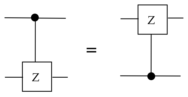
- Similarly, the upside-down version is:
$$
\bar{C}_{\scriptsize Z}
\eql
I \otimes \otr{0}{0} \; + \; Z \otimes \otr{1}{1}
$$
- Surprisingly,
\(\bar{C}_{\scriptsize Z} = \cz\):
- \(\cnot\) can be built out of \(\cz\) and two 1-qubit Hadamards:
- In some hardware platforms, \(\cz\) is easier to implement.
- Some books use \(C_{\scriptsize SIGN}\) as an alternate
name for \(\cz\).
In-Class Exercise 11:
Use matrices or Dirac forms to show both results above:
- \(\bar{C}_{\scriptsize Z} = \cz\)
- \(\cnot = (I\otimes H) \cz (I\otimes H) \)
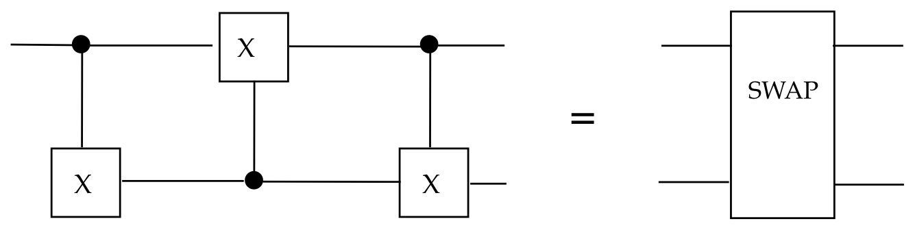
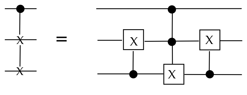
The SWAP gate:
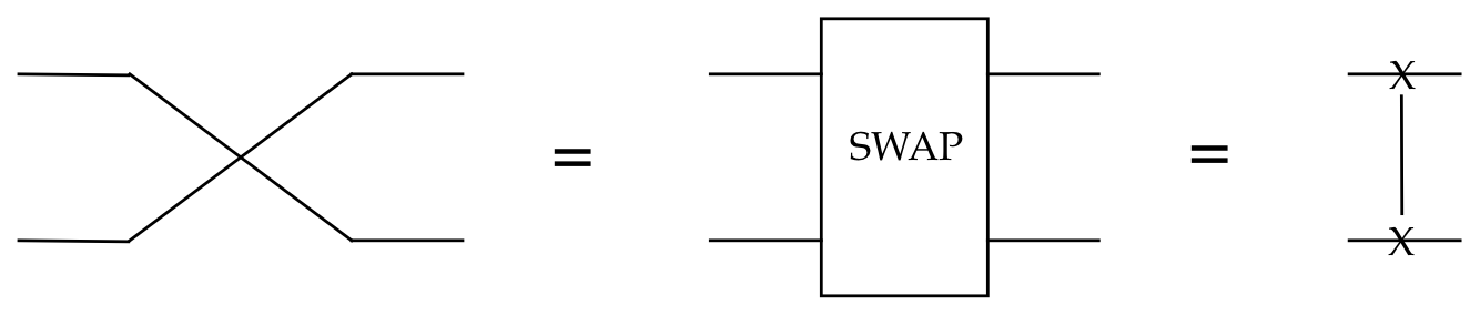
In-Class Exercise 12:
- Use matrix forms to show
\(\mbox{SWAP} = \cnot \bar{C}_{\scriptsize NOT} \cnot\)
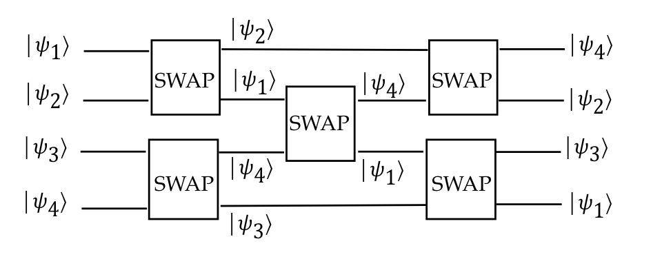
- Sketch the staged circuit for swapping the first and
eighth qubits. (Your drawing can be rough, and scanned from paper.)
- With \(n=2^m\) qubits, how many SWAP gates are needed
to swap the first and last qubits?
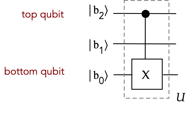
Compact notation when the input is a standard-basis vector:
- We can describe the four 2-qubit standard basis vectors as:
$$
\setl{ \kt{b_1, b_0}: \;\; b_i \in \{0,1\} }
$$
That is,
$$\eqb{
\kt{00} & \mbx{\(b_1=0, b_0=0\)} \\
\kt{01} & \mbx{\(b_1=0, b_0=1\)} \\
\kt{10} & \mbx{\(b_1=1, b_0=0\)} \\
\kt{11} & \mbx{\(b_1=1, b_0=1\)} \\
}$$
- While the binary variables \(b_1, b_0\) make the right-to-left
order clear, it's just as common to use any variables, as in:
$$
\setl{ \kt{x, y}: \;\; x,y \in \{0,1\} }
$$
- Then, the effect of \(\cnot\) on the S-basis vectors can:
be written as:
$$
\cnot \kt{b_1, b_0} \eql \kt{b_1, b_1\oplus b_0}
$$
or
$$
\cnot \kt{xy} \eql \kt{x, x\oplus y}
$$
where \(\oplus\) is the binary XOR operator.
- To see how this works for \(\cnot\),
let's write out the four cases:
$$\eqb{
\cnot \kt{00} & \eql & \kt{0, 0 \oplus 0} & \eql & \kt{00}\\
\cnot \kt{01} & \eql & \kt{0, 0 \oplus 1} & \eql & \kt{01}\\
\cnot \kt{10} & \eql & \kt{1, 1 \oplus 0} & \eql & \kt{11}\\
\cnot \kt{11} & \eql & \kt{1, 1 \oplus 1} & \eql & \kt{10}\\
}$$
- Similarly, recalling that
$$\eqb{
\cz \kt{00} & \eql & \kt{00} \\
\cz \kt{01} & \eql & \kt{01} \\
\cz \kt{10} & \eql & \kt{10} \\
\cz \kt{11} & \eql & -\kt{11} \\
}$$
we can write \(\cz\) more compactly with this notation as:
$$
\cz \kt{b_1, b_0} \eql (-1)^{b_1b_0} \kt{b_1, b_0}
$$
or
$$
\cz \kt{x}\kt{y} \eql (-1)^{xy} \kt{x}\kt{y}
$$
where, for example, \(xy\) uses the binary AND operation.
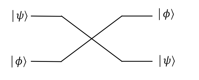
- SWAP of course can be trivially written for S-basis vectors as:
$$
\mbox{SWAP} \kt{x}\kt{y} \eql \kt{y}\kt{x}
$$
Sometimes, this is shortened to \(\mbox{SWAP} \kt{xy} \eql \kt{yx}\).
- Such binary-variable usage is especially valuable when
exploiting known results from the world of binary operations, such as:
- \(x \oplus x = 0\)
- \(x \oplus 0 = x\)
- \(x \oplus y = y \oplus x\)
- \((x \oplus y) \oplus z = x \oplus (y \oplus z) \)
(See
solved problems
for an example.)
6.10
Multiply-controlled gates
The overall goal:
- Apply a gate to the k-th qubit only when other qubits are in a
certain state.
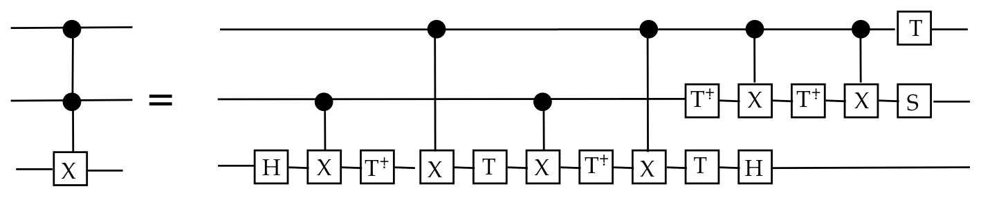
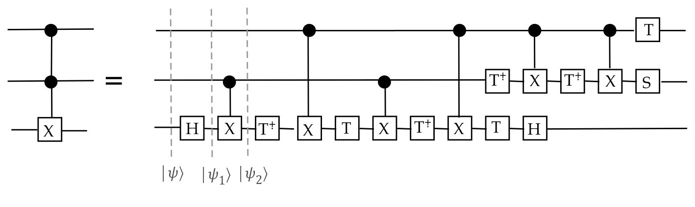
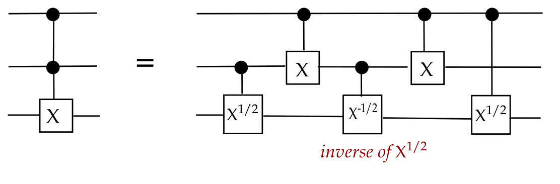
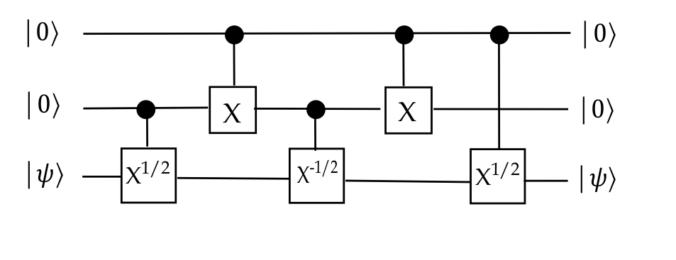
Let's first examine one of the most important such gates:
\(\ccnot\)
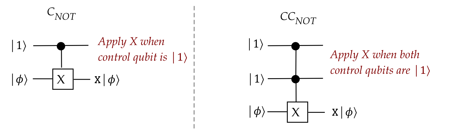
- Suppose we want a 3-qubit gate where the first two qubits
"control" the third, as shown on the right.
- In this case, what we seek is:
- When the first two qubits both have state \(\kt{1}\),
then "flip" (apply \(X\) to) the third.
- In all other cases, leave the third qubit as is.
- And: the control qubits are unchanged.
- We can write this as:
$$\eqb{
\ccnot \ksi & \eql & \ksi
& \;\;\;\;\;\; & \ksi \in \parenl{
\kt{000}, \kt{001}, \kt{010}, \kt{011}, \kt{100}, \kt{101}
} \\
\ccnot \kt{110} & \eql & \kt{111} & & \\
\ccnot \kt{111} & \eql & \kt{110} & & \\
}$$
- Thus,
$$\eqb{
& \; &
\ccnot \\
& \; &
\eql
\otr{000}{000} + \ldots + \otr{101}{101}
+ {\bf \otr{110}{111} } + {\bf \otr{111}{110} } \\
& \; &
\eql
\mat{
1 & 0 & 0 & 0 & 0 & 0 & 0 & 0 \\
0 & 1 & 0 & 0 & 0 & 0 & 0 & 0 \\
0 & 0 & 1 & 0 & 0 & 0 & 0 & 0 \\
0 & 0 & 0 & 1 & 0 & 0 & 0 & 0 \\
0 & 0 & 0 & 0 & 1 & 0 & 0 & 0 \\
0 & 0 & 0 & 0 & 0 & 1 & 0 & 0 \\
0 & 0 & 0 & 0 & 0 & 0 & 0 & {\bf 1} \\
0 & 0 & 0 & 0 & 0 & 0 & {\bf 1} & 0 \\
}
}$$
- Of course, just because we make up a unitary operation
doesn't necessarily mean it's easy to implement in real hardware.
\(\rhd\)
We'll address this issue in a later section in this module
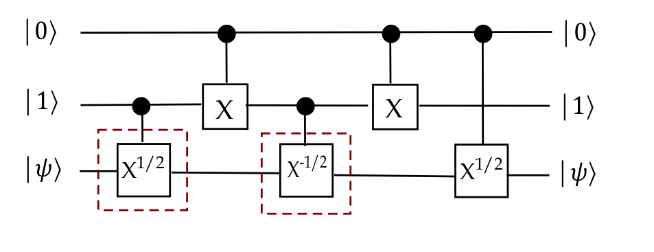
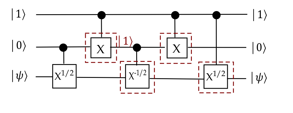
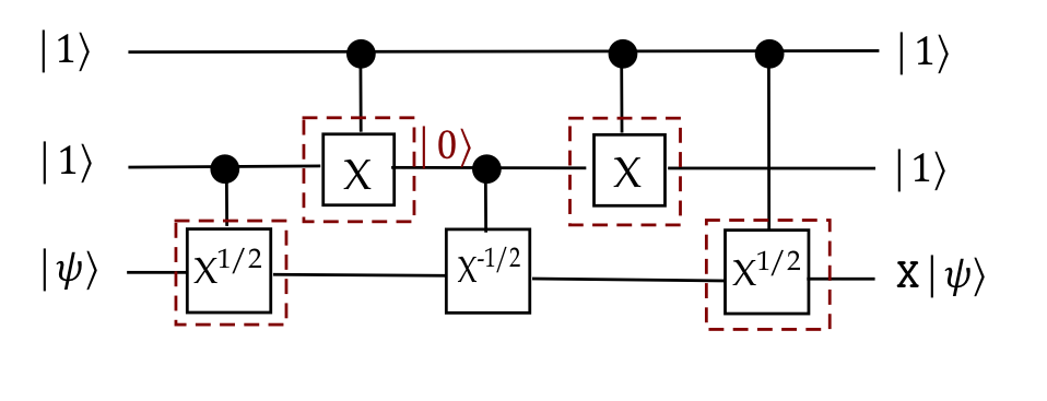
- Once we have such a gate, one can use additional gates
to specify other types of control:
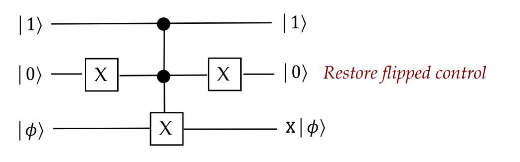
- For example, suppose we want to apply \(X\) to the third
qubit when the first two are in state \(\kt{10}\).
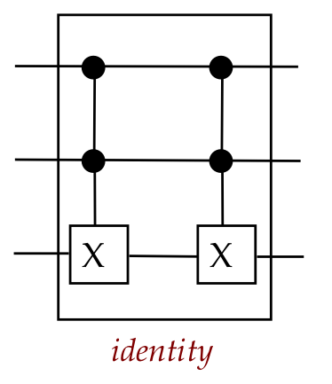
- In this case one can add an \(X\) before the 2nd qubit:
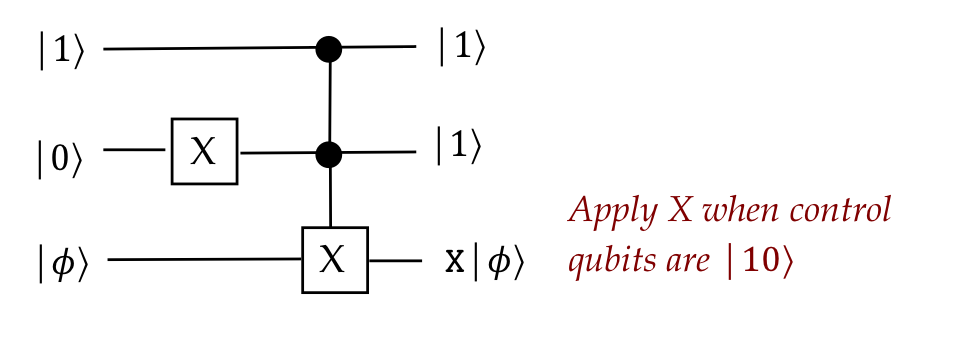
- Notice that the second control bit was modified. To restore,
one can "undo" the \(X\) on the second bit:
- Note:
- The "control" has been set up for standard basis vectors.
- However, the third qubit can be in any state.
- Of course, nothing prevents us from applying the circuit
to arbitrary vectors, if that's useful.
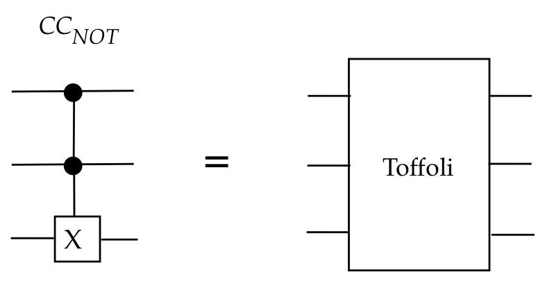
- Terminology: \(\ccnot\) = Controlled-controlled-NOT
6.11
Common 3-qubit gates
We've already seen the first important 3-qubit gate,
\(\ccnot\), also known as the Toffoli gate:
The Fredkin gate:
In-Class Exercise 13:
Complete the remaining two steps in showing
\(
\parenl{I \otimes \bar{C}_{\scriptsize NOT} }
\ccnot
\parenl{I \otimes \bar{C}_{\scriptsize NOT} }
\).
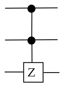
The \(\ccz\) gate:
6.12
A useful trick: control vector conversion
In some applications, it's useful to be able
to transform an output vector so that controls
can be applied in a certain pre-configured way.
For example, in a 3-qubit case,
suppose the input is known to be \(\kt{001}\) and
we want to convert this to \(\kt{000}\):
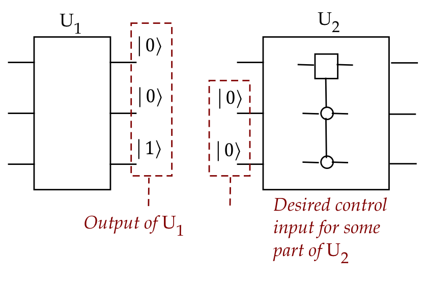
- In this case, the \(\kt{001}\) is the output of some circuit
\(U_1\).
- The circuit \(U_2\) needs the latter 2 bits
of the input to be \(\kt{x00}\),
where \(x\) is either 0 or 1.
- This can be achieved through a \(\cnot\):
- Note: the control state is \(\kt{0}\).
- Why don't we simply apply \(X\) to the 3rd qubit?
- Our goal is to have this transformation apply only
when the input is \(\kt{x01}\) (latter two in state \(\kt{01}\).
- Then, other inputs will not be affected.
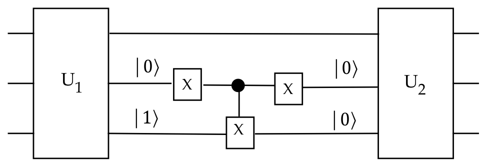
Next, suppose we wish to convert \(\kt{x01}\) to
\(\kt{x10}\):
- In this case, a single bit-flip amongst the 2nd and 3rd
qubits is not sufficient.
- We can instead use two \(\cnot\) gates.
- To do this, we first flip one state bit (3rd qubit) going from
\(\kt{x01} \rightarrow \kt{x00}\).
- And then \(\kt{x00} \rightarrow \kt{x10}\).
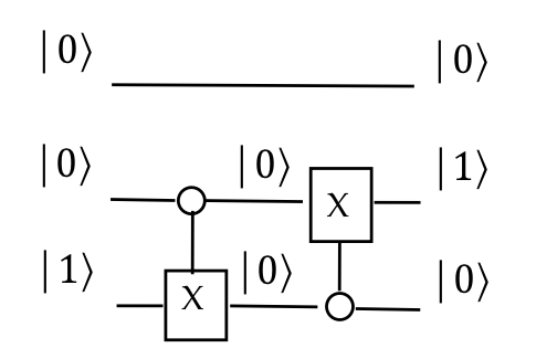
- Notice that our drawing now reflects the use of
\(\kt{0}\) as control (open circle in the drawing).
- In general, several steps may be needed to flip one bit at a
time to transition from one set of input qubits to another with
desired controls.
- For example, suppose one wants to convert \(\kt{100x}\)
to \(\kt{011x}\).
- Then, the following steps would work:
$$
\kt{100x} \rightarrow \kt{000x}
\rightarrow \kt{010x}
\rightarrow \kt{011x}
$$
- Each step is a controlled-flip, controlled by two amongst
the (first) three bits involved.
In-Class Exercise 14:
Draw the circuit that
converts \(\kt{100x}\) to \(\kt{011x}\).
6.13
Notation for gates that act on spread-apart qubits
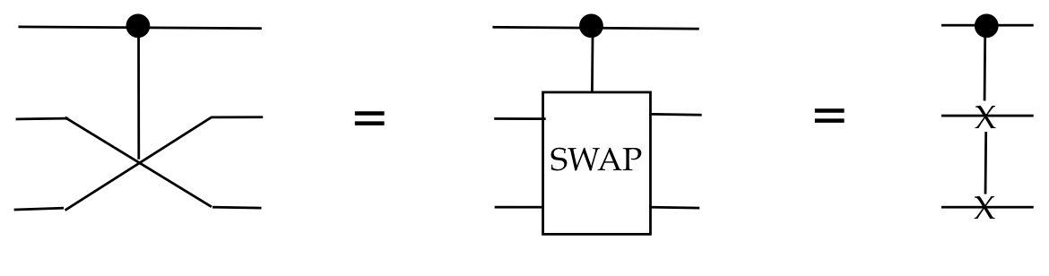
Thus far, in our examples, multi-qubit gates have acted on
neighboring qubits, as in:
But it's often the case that we need a gate to act "long distance",
between qubits that are spread apart, as in:
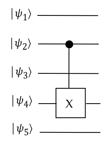
The purpose of this section is to get familiar with Dirac notation
that's often used for such cases:
- We will use the subscript \(j\) with a unitary to indicate that
it's acting on the \(j\)-th qubit.
- For example, \(I_2\) is the identity on the second qubit,
and \(X_4\) is the \(X\) gate applied to the \(4\)-the qubit.
- Consider now the \(\cnot\) gate applied to the first two qubits:
- In Dirac form, the gate is written as:
$$
\cnot \eql \otr{0}{0} \otimes I \, + \, \otr{1}{1} \otimes X
$$
- To clarify which qubits, we can add the subscript:
$$
\cnot \eql \otr{0}{0}_1 \otimes I_2 \, + \, \otr{1}{1}_1 \otimes X_2
$$
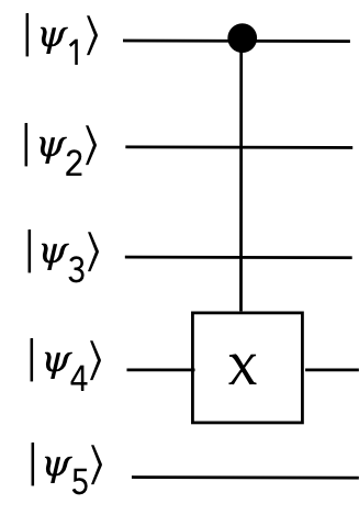
- Now consider a \(\cnot\) that uses qubit 1 as the control,
and qubit 3 as the target:
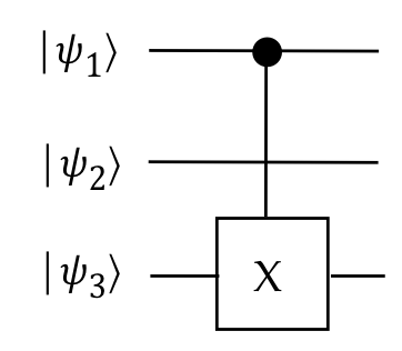
- Since nothing is done to the 2nd qubit, we need \(I_2\) in
the second tensor spot.
- Thus, the entire 3-qubit unitary is written as:
$$
U \eql
\otr{0}{0}_1 \otimes I_2 \otimes I_3
\, + \, \otr{1}{1}_1 \otimes I_2 \otimes X_3
$$
- To see this at work, let's apply \(U\) to \(\kt{010}\)
and \(\kt{110}\) as examples:
- First, \(U\kt{010}\):
$$\eqb{
U\kt{010}
& \eql &
\parenl{ \otr{0}{0}_1 \otimes I_2 \otimes I_3
\, + \, \otr{1}{1}_1 \otimes I_2 \otimes X_3 } \, \kt{010} \\
& \eql &
\parenl{ \otr{0}{0}_1 \otimes I_2 \otimes I_3
\, + \, \otr{1}{1}_1 \otimes I_2 \otimes X_3 } \, \kt{0}\kt{1}\kt{0} \\
& \eql &
\parenl{ \otr{0}{0}_1 \kt{0} \otimes I_2 \kt{1} \otimes I_3 \kt{0}
\, + \, \otr{1}{1}_1 \kt{0} \otimes I_2 \kt{1}\otimes X_3\kt{0} }\\
& \eql &
\otr{0}{0}_1 \kt{0} \otimes I_2 \kt{1} \otimes I_3 \kt{0} \\
& \eql &
\kt{0} \otimes \kt{1} \otimes \kt{0} \\
& \eql &
\kt{010}
}$$
Notice how the term \(\otr{1}{1}_1 \kt{0} = 0\) eliminates the
entire tensor product \(\otr{1}{1}_1 \kt{0} \otimes I_2 \kt{1}\otimes X_3\kt{0}\).
- Similarly,
$$\eqb{
U\kt{110}
& \eql &
\parenl{ \otr{0}{0}_1 \otimes I_2 \otimes I_3
\, + \, \otr{1}{1}_1 \otimes I_2 \otimes X_3 } \, \kt{110} \\
& \eql &
\parenl{ \otr{0}{0}_1 \otimes I_2 \otimes I_3
\, + \, \otr{1}{1}_1 \otimes I_2 \otimes X_3 } \, \kt{1}\kt{1}\kt{0} \\
& \eql &
\parenl{ \otr{0}{0}_1 \kt{1} \otimes I_2 \kt{1} \otimes I_3 \kt{0}
\, + \, \otr{1}{1}_1 \kt{1} \otimes I_2 \kt{1}\otimes X_3\kt{0} }\\
& \eql &
\otr{1}{1}_1 \kt{1} \otimes I_2 \kt{1}\otimes X_3\kt{0}\\
& \eql &
\kt{1} \otimes \kt{1} \otimes \kt{1} \\
& \eql &
\kt{111}
}$$
- We can now see how to generalize to a \(\cnot\) that applies
to qubits \(j\) and \(k\):
- Let \(C_{j,k}\) be a \(\cnot\) gate that uses \(j\) as the
control for qubit \(k\).
- For now, let's assume \(j \lt k\).
- Then
$$\eqb{
C_{j,k}
& \eql &
I_1 \otimes \ldots \otimes I_{j-1}
\otimes {\bf \otr{0}{0}_j}
\otimes I_{j+1} \otimes \ldots \otimes I_{k-1}
\otimes {\bf I_{k}}
\otimes I_{k+1} \otimes \ldots \otimes I_{n} \\
& \; &
\;\; + \;\;
I_1 \otimes \ldots \otimes I_{j-1}
\otimes {\bf \otr{1}{1}_j}
\otimes I_{j+1} \otimes \ldots \otimes I_{k-1}
\otimes {\bf X_{k}}
\otimes I_{k+1} \otimes \ldots \otimes I_{n}
}$$
where we can see the action of \(\cnot\) on the two qubits \(j,k\).
- For example, in a 5-qubit case, \(C_{2,4}\) is written as:
$$\eqb{
C_{2,4}
& \eql &
I_1 \otimes {\bf \otr{0}{0}_2} \otimes I_3 \otimes {\bf I_4}
\otimes I_5 \\
& &
+ \; I_1 \otimes {\bf \otr{1}{1}_2} \otimes I_3 \otimes {\bf X_4}
\otimes I_5 \\
}$$
In-Class Exercise 15:
Write down the matrix and Dirac versions of
a 2-qubit controlled-\(P(\theta)\) gate acting on qubits 1 and 2.
Then, show how this can be written for qubits \(j\) and \(k\) where
\(j\) is the control qubit.
6.14
Qubit-labeling conventions
Let's go back to this example:
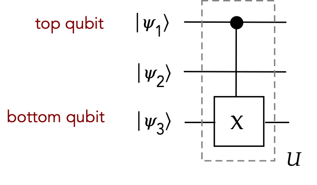
And write the resulting 3-qubit unitary as:
$$
U \eql
\otr{0}{0}_1 \otimes I_2 \otimes I_3
\, + \, \otr{1}{1}_1 \otimes I_2 \otimes X_3
$$
When applied to the input, this would look like:
$$
U \kt{\psi_1}\kt{\psi_2}\kt{\psi_3}
\eql
\parenl{
\otr{0}{0}_1 \otimes I_2 \otimes I_3
\, + \, \otr{1}{1}_1 \otimes I_2 \otimes X_3}
\: \kt{\psi_1}\kt{\psi_2}\kt{\psi_3}
$$
Notice the following about the indexing in the expression and the
circuit diagram:
- The qubits go left to right in increasing
qubit number in the expression:
- The leftmost qubit in the expression \(\kt{\psi_1}\kt{\psi_2}\kt{\psi_3}\) is the one with
the smallest index \(\kt{\psi_1}\).
- This is natural for us, mathematically.
- In the diagram, the numbering increases from top to bottom:
- The topmost qubit is the lowest numbered one.
- That is, \(\kt{\psi_1}\) is at the top.
This may or may not be "natural", depending on your point of view.
- We'll call this the top-down style.
- Most books use this style (except for one prominent one)
except when using binary variables.
Bottom-up convention using binary variables:
6.15
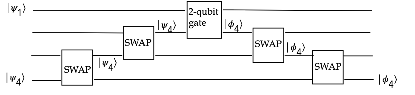
Using SWAP to move qubit states
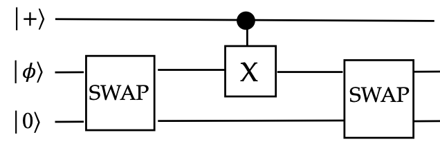
Consider again the problem of applying a 2-qubit gate
to qubits that are physically spread apart:
- In practice, typically, it is not possible to apply at long distance.
- In some architectures, 2-qubit gates can only be applied
to physically adjacent qubits.
- A common solution is to apply a series of SWAPs to make
two qubits adjacent, and then repeat the SWAPs to restore
their original position.
- However, we should examine whether entanglement
prohibits swapping from working.
Let's look a simple example with \(\cnot\):
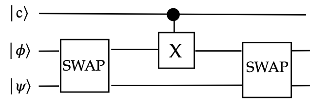
- Here
- \(\kt{c} \in \setl{ \kt{0}, \kt{1} }\)
- We wish to apply \(\cnot\) from the first (as control)
to the third.
- Consider the case when \(\kt{c} = \kt{0}\)
- The first 3-qubit unitary then applies as
$$
\parenl{I \otimes \mbox{SWAP}} \kt{0}\kt{\phi}\ksi
\eql \kt{0}\ksi\kt{\phi}
$$
- Then \(\cnot\) applies to this state:
$$
\parenl{\cnot \otimes I} \kt{0}\ksi\kt{\phi}
\eql \kt{0}\ksi\kt{\phi}
$$
- Recall what \(\cnot\) does to a generic
state:
$$\eqb{
\cnot \parenl{ \kt{0} \otimes (\alpha\kt{0} + \beta\kt{1}) }
& \eql & \kt{0} \otimes (\alpha\kt{0} + \beta\kt{1}) \\
\cnot \parenl{ \kt{1} \otimes (\alpha\kt{0} + \beta\kt{1}) }
& \eql & \kt{1} \otimes (\beta\kt{0} + \alpha\kt{1}) \\
}$$
- Returning to the circuit, we apply the second SWAP:
$$
\parenl{I \otimes \mbox{SWAP}} \kt{0}\ksi\kt{\phi}
\eql \kt{0}\kt{\phi}\ksi
$$
- Thus, the third qubit is in the desired state.
- Next: \(\kt{c} = \kt{1}\)
- Suppose
$$
\kt{\psi^\prime} \eql X\ksi \eql \beta\kt{0} + \alpha\kt{1}
$$
- Then, condensing the steps
$$\eqb{
& & \hspace{-20pt}
\parenl{I \otimes \mbox{SWAP}}
\parenl{\cnot \otimes I}
\parenl{I \otimes \mbox{SWAP}}
\parenl{ \kt{1}\kt{\phi}\ksi } \\
& \eql &
\parenl{I \otimes \mbox{SWAP}}
\parenl{\cnot \otimes I}
\parenl{ \kt{1}\ksi\kt{\phi} } \\
& \eql &
\parenl{I \otimes \mbox{SWAP}}
\parenl{ \kt{1}\kt{\psi^\prime}\kt{\phi} } \\
& \eql &
\kt{1}\kt{\phi} \kt{\psi^\prime} \\
}$$
Which is the desired state.
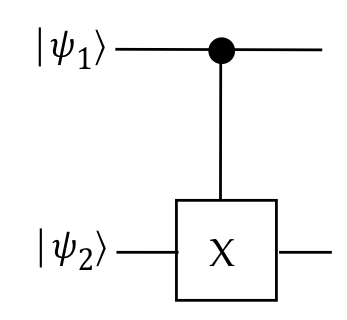
Does this work if we seek to entangle with \(\cnot\)?
In-Class Exercise 16:
(Optional for submission)
Consider this circuit:
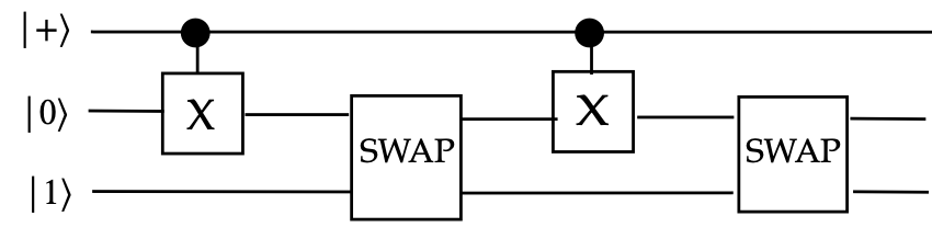
What is the resulting 3-qubit state? Which qubits, if any,
are entangled?
6.16
Caveats
First, as we've seen before, the notion of "control" can
be ambiguous:
One needs to be careful in reasoning about global versus
local phase in the multi-qubit context:
- Consider the difference between \(\kt{1} \otimes \kt{0}\)
and \(\kt{1} \otimes K(\delta) \kt{0}\):
- We may reason that
$$
K(\delta) \kt{0} \eql e^{i\delta} \kt{0} \eql \kt{0}
$$
because of global-phase.
- Then
$$
\kt{1} \otimes K(\delta) \kt{0}
\eql
\kt{1} \otimes \kt{0}
\eql \kt{10}
$$
with this reasoning.
- Now let's apply tensoring properties
$$
\kt{1} \otimes K(\delta) \kt{0}
\eql
K(\delta) \parenl{ \kt{1} \otimes \kt{0} }
\eql
e^{i\delta} \parenl{ \kt{1} \otimes \kt{0} }
\eql
e^{i\delta} \kt{10}
\eql
\kt{10}
$$
So it appears to work in this case.
- However, if instead this was part of an entangled superposition:
$$
\isqts{1} \parenl{ I \kt{01} + \kt{1} \otimes K(\delta) \kt{0} }
\eql
\isqts{1} \parenl{ \kt{01} + e^{i\delta} \kt{10} }
\; \neq \;
\isqts{1} \parenl{ \kt{01} + \kt{10} }
$$
In this case, the factor \(e^{i\delta}\) cannot be ignored.
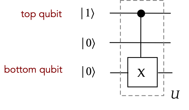
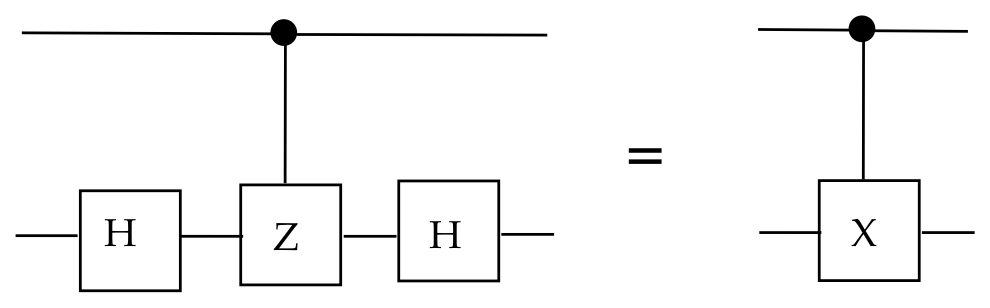
One cannot treat quantum circuits like classical circuits
even with standard-basis qubits:
- Consider this example:
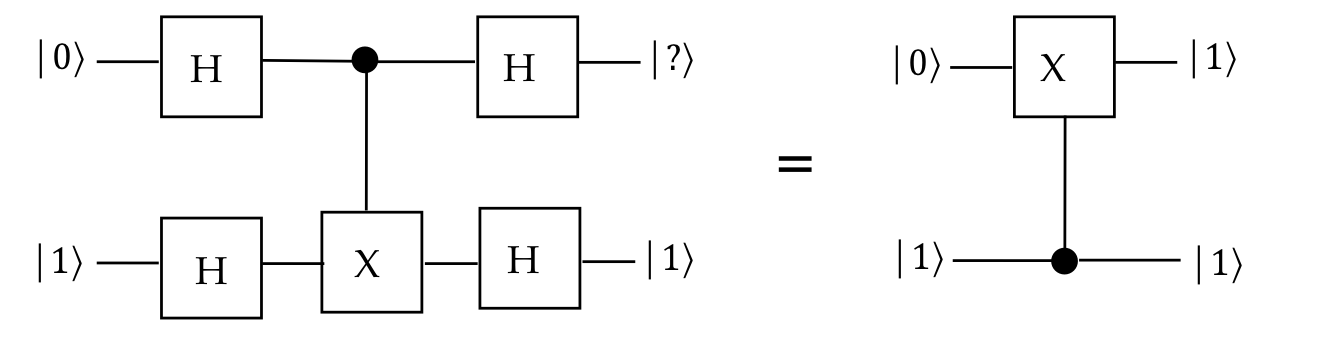
- For the top qubit on the left, it's tempting to reason
that:
- The control "dot" does nothing to change it.
- The two Hadamards in sequence amount to \(H H = H^2 = I\).
- That is, they won't have an effect on the top qubit.
- So, in the diagram, the top qubit should remain \(\kt{0}\)
by this reasoning.
- But that is false, as seen by the equivalency on the right.
- Recall that \(\cnot\) cannot be decomposed into smaller
tensored unitaries, and it can entangle, even if not apparent.
- Thus, the only way to reason is to work through circuits.
- For larger circuits, it's best to use a simulator to verify.
Don't forget: Module-6 solved problems