Problem:
Derive the matrix for \(R_Y(\theta)\).
Solution:
$$\eqb{
R_Y(\theta) & \eql & e^{\frac{-i\theta}{2}Y} \\
& \eql &
I\cos\frac{\theta}{2} - iY\sin\frac{\theta}{2} \\
& \eql &
\mat{\cos\frac{\theta}{2} & 0 \\ 0 & \cos\frac{\theta}{2}}
- i\sin\frac{\theta}{2}
\mat{0 & -i\\ i & 0} \\
& \eql &
\mat{\cos\frac{\theta}{2} & 0 \\ 0 & \cos\frac{\theta}{2}}
+
\mat{0 & -\sin\frac{\theta}{2} \\ \sin\frac{\theta}{2} & 0} \\
& \eql &
\mat{\cos\frac{\theta}{2} & -\sin\frac{\theta}{2} \\
\sin\frac{\theta}{2} & \cos\frac{\theta}{2} }
}$$
Problem:
Show that
$$
\sqrt{X} \eql
\frac{1}{2}
\mat{1+i & 1-i\\
1-i & 1+i}
$$
Solution:
Using the approach shown for powers of Pauli matrices,
$$\eqb{
X^{\frac{1}{2}}
& \eql &
e^{i \frac{\pi}{4} }
e^{-i \frac{\pi}{4} X} \\
& \eql &
e^{i \frac{\pi}{4} }
e^{-i \frac{\pi}{4} X} \\
& \eql &
e^{i \frac{\pi}{4} }
\left( I\cos\frac{\pi}{4} - iX \sin\frac{\pi}{4} \right) \\
& \eql &
e^{i \frac{\pi}{4} }
\left(
\mat{ \isqt{1} & 0 \\ 0 & \isqt{1} }
- i \mat{ 0 & \isqt{1} \\ \isqt{1} & 0 }
\right) \\
& \eql &
\parenl{ \isqt{1} + \isqt{i} }
\left(
\mat{ \isqt{1} & -\isqt{i} \\
-\isqt{i} & \isqt{1} }
\right) \\
& \eql &
\frac{1}{2}
\parenl{ 1 + i }
\left(
\mat{ 1 & -i \\
-i & 1 }
\right) \\
& \eql &
\frac{1}{2}
\mat{1+i & 1-i\\
1-i & 1+i}
}$$
Problem:
For a 1-qubit operator such that \(A^2=I\) show that
\( \left( e^{i\theta A} \right)^\dagger = e^{-i\theta A^\dagger} \)
and use this to show that \(R_X(\theta)\) is not Hermitian.
Solution:
$$\eqb{
\left( e^{i\theta A} \right)^\dagger
& \eql &
\parenl{ I\cos\theta }^\dagger
+ \parenl{ iA\sin\theta }^\dagger \\
& \eql &
I\cos\theta + (i)^* \sin\theta A^\dagger \\
& \eql &
I\cos\theta - i \sin\theta A^\dagger \\
& \eql &
e^{-i\theta A^\dagger}
}$$
Thus,
$$\eqb{
R_X(\theta)^\dagger
& \eql &
\left( e^{i\theta X} \right)^\dagger \\
& \eql &
e^{-i\theta X^\dagger} \\
& \eql &
e^{-i\theta X}
& \neq &
e^{i\theta X}
}$$
Problem:
Show that \(H = K(-\frac{\pi}{4})\, X \, Y^{\frac{1}{2}}\)
Solution:
$$
X \, Y^{\frac{1}{2}}
\eql
\mat{0 & 1\\ 1 & 0}
e^{\frac{\pi}{4}}
\mat{1 & -1\\ 1 & 1}
\eql
e^{\frac{\pi}{4}}
\mat{1 & 1\\ 1 & -1}
\eql
e^{\frac{\pi}{4}}
H
$$
Hence, a correcting global phase of \(K(-\frac{\pi}{4})\)
results in \(H\).
Problem:
Recall that the \(P(\theta)\) gate was used in setting
a qubit's state to a desired state \(\alpha\kt{0}+\beta\kt{1}\).
Show how the \(R_Z(\theta)\) gate instead of the \(P(\theta)\) gate
can be used for the same purpose of setting qubit
Solution:
Recall that we converted to polar form and wrote:
$$
\alpha\kt{0}+\beta\kt{1}
\eql
r_1\kt{0} + r_2 e^{i\theta_2-\theta_1}\kt{1}
$$
where
$$\eqb{
\alpha & \eql & r_1 e^{i\theta_1} \\
\beta & \eql & r_2 e^{i\theta_2} \\
}$$
And then we showed that
$$
R_Y(2\cos^{-1}\alpha) \kt{0}
\eql r_1\kt{0} + r_2 \kt{1}
$$
Next, let's recall $$ R_Z(2\phi) \eql \mat{ e^{-i\phi} & 0\\ 0 & e^{i\phi} } $$ and apply $$\eqb{ R_Z(2\phi) R_Y(2\cos^{-1}\alpha) \kt{0} & \eql & R_Z(2\phi) \parenl{ r_1\kt{0} + r_2 \kt{1}} \\ & \eql & \mat{ e^{-i\phi} & 0\\ 0 & e^{i\phi} } \mat{r_1\\ r_2}\\ & \eql & e^{-i\phi} r_1 \kt{0} + e^{i\phi} r_2 \kt{1} \\ & \eql & e^{-i\phi} \parenl{ r_1 \kt{0} + e^{i2\phi} r_2 \kt{1} } \\ }$$ By choosing \(2\phi = \theta_2-\theta_1\), and ignoring the global phase, we have $$ R_Z(2\phi) R_Y(2\cos^{-1}\alpha) \kt{0} \eql \alpha\kt{0} + \beta\kt{1} $$ as desired.
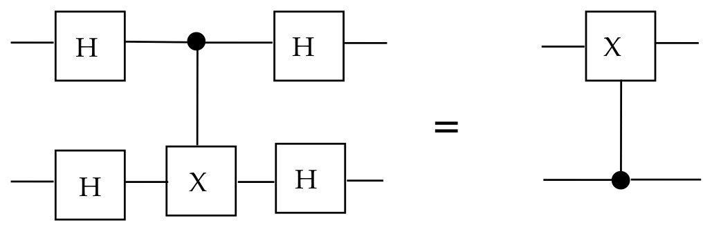
Problem:
Show that
Solution:
Let's start by computing \(H\otimes H\):
$$
H\otimes H \eql \frac{1}{2}
\mat{1 & 1 & 1 & 1\\
1 & -1 & 1 & -1\\
1 & 1 & -1 & -1\\
1 & -1 & -1 & 1}
$$
Then
$$
\cnot (H\otimes H) \eql \frac{1}{2}
\mat{1 & 0 & 0 & 0\\
0 & 1 & 0 & 0\\
0 & 0 & 0 & 1\\
0 & 0 & 1 & 0}
\mat{1 & 1 & 1 & 1\\
1 & -1 & 1 & -1\\
1 & 1 & -1 & -1\\
1 & -1 & -1 & 1}
\eql
\mat{1 & 1 & 1 & 1\\
1 & -1 & 1 & -1\\
1 & -1 & -1 & 1\\
1 & 1 & -1 & -1}
$$
And finally,
$$
(H\otimes H) \cnot (H\otimes H)
\eql
\frac{1}{4}
\mat{1 & 1 & 1 & 1\\
1 & -1 & 1 & -1\\
1 & 1 & -1 & -1\\
1 & -1 & -1 & 1}
\mat{1 & 1 & 1 & 1\\
1 & -1 & 1 & -1\\
1 & -1 & -1 & 1\\
1 & 1 & -1 & -1}
\eql
\frac{1}{4}
\mat{4 & 0 & 0 & 0\\
0 & 0 & 0 & 4\\
0 & 0 & 4 & 0\\
0 & 4 & 0 & 0}
$$
Which gives the desired result
$$
\bar{C}_{\scriptsize NOT}
\eql
\mat{1 & 0 & 0 & 0\\
0 & 0 & 0 & 1\\
0 & 0 & 1 & 0\\
0 & 1 & 0 & 0}
$$
Problem:
Recall the example from the section on applying SWAP to move
qubits and now suppose we measure the first qubit in
standard basis:
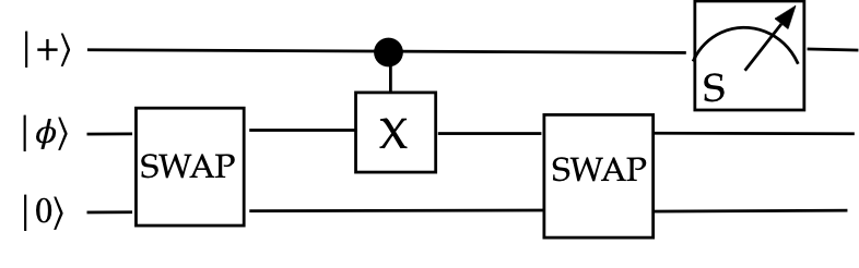
How does this impact the second qubit? The third qubit?
Solution:
Recall that the circuit, just before measurement, produces the
3-qubit state
$$
\ksi \eql
\isqts{1} \parenl{ \kt{0}\kt{\phi}\kt{0} + \kt{1}\kt{\phi}\kt{1} }
$$
There are two projectors here:
$$\eqb{
P_0 & \eql & \otr{0}{0} \otimes I \otimes I \\
P_1 & \eql & \otr{1}{1} \otimes I \otimes I \\
}$$
Applying each gives
$$\eqb{
P_0
\isqts{1} \parenl{ \kt{0}\kt{\phi}\kt{0} + \kt{1}\kt{\phi}\kt{1} }
& \eql & \isqts{1} \kt{0}\kt{\phi}\kt{0} \\
P_1
\isqts{1} \parenl{ \kt{0}\kt{\phi}\kt{0} + \kt{1}\kt{\phi}\kt{1} }
& \eql & \isqts{1} \kt{1}\kt{\phi}\kt{1} \\
}$$
From which we get
$$\eqb{
\mbox{Outcome } \kt{0}\kt{\phi}\kt{0} &
\mbox{ with probability } \smf{1}{2} \\
\mbox{Outcome } \kt{1}\kt{\phi}\kt{1} &
\mbox{ with probability } \smf{1}{2} \\
}$$
As we can see, the third qubit is affected while the second is not.
Problem:
Show that three \(\cnot\)'s can be combined to create
SWAP as follows:
$$
\mbox{SWAP} \eql \cnot \bar{C}_{\scriptsize NOT} \cnot
$$
That is,
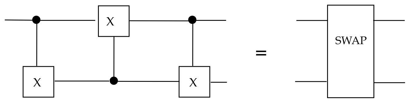
Solution:
Here, we will exploit both the compactness of binary-variable
notation and known properties of the \(\oplus\) binary operator.
Let \(x,y\) be two binary variables, i.e., \(x,y\in\{0,1\}\). Then, for any values of \(x,y\), the 2-qubit vector \(\kt{x}\kt{y}\) is a standard-basis vector. Let's apply the circuit on the right to \(\kt{x}\kt{y}\): $$\eqb{ \parenl{\cnot \bar{C}_{\scriptsize NOT} \cnot} \: \kt{x}\kt{y} & \eql & \parenl{\cnot \bar{C}_{\scriptsize NOT} } \cnot \kt{x}\kt{y} & \mbx{First: the leftmost gate}\\ & \eql & \parenl{\cnot \bar{C}_{\scriptsize NOT} } \kt{x}\kt{x \oplus y} & \mbx{Apply \(\cnot\)} \\ & \eql & \parenl{\cnot } \bar{C}_{\scriptsize NOT} \kt{x}\kt{x \oplus y} & \mbx{Next gate}\\ & \eql & \parenl{\cnot } \kt{(x \oplus y) \oplus x}\kt{x \oplus y} & \mbx{Apply reverse \(\cnot\)}\\ & \eql & \parenl{\cnot } \kt{x \oplus (x \oplus y) }\kt{x \oplus y} & \mbx{Properties of XOR}\\ & \eql & \cnot \kt{y}\kt{x \oplus y} & \mbx{Properties of XOR}\\ & \eql & \kt{y}\kt{y\oplus (x \oplus y)} & \mbx{Apply third gate}\\ & \eql & \kt{y}\kt{(x \oplus y) \oplus y} & \mbx{Properties of XOR}\\ & \eql & \kt{y}\kt{x}\\ }$$ It is common to shorten the steps in the following way: $$\eqb{ \kt{x}\kt{y} & \xrightarrow{\cnot} & \kt{x}\kt{x \oplus y} \\ & \xrightarrow{\bar{C}_{\scriptsize NOT}} & \kt{y}\kt{x \oplus y} \\ & \xrightarrow{\cnot} & \kt{y}\kt{x} }$$ (But this obscures some of the binary operator simplifications)
Thus, if $$ U \eql \parenl{\cnot \bar{C}_{\scriptsize NOT} \cnot} $$ then we've shown that $$ U\kt{x}\kt{y} \eql \kt{y}\kt{x} $$ for the standard-basis vectors. Does this mean it'll work for any tensored 2-qubit vectors? That is, is it true that $$ U \kt{\psi}\kt{\phi} \eql \kt{\phi}\kt{\psi}? $$ Here, we'll exploit linearity to show that this is true. Let $$\eqb{ \ksi & \eql & \alpha_1 \kt{0} + \alpha_2 \kt{1} \\ \khi & \eql & \beta_1 \kt{0} + \beta_2 \kt{1} \\ }$$ Then, $$\eqb{ \parenl{ \alpha_1 \kt{0} + \alpha_2 \kt{1} } \otimes \parenl{ \beta_1 \kt{0} + \beta_2 \kt{1} } & \xrightarrow{\text{expand}}& \alpha_1\beta_1 \kt{00} + \alpha_1\beta_2 \kt{01} \alpha_2\beta_1 \kt{10} + \alpha_2\beta_2 \kt{11} \\ & \xrightarrow{U} & \beta_1\alpha_1 \kt{00} + \beta_1\alpha_2 \kt{01} \beta_2\alpha_1 \kt{10} + \beta_2\alpha_2 \kt{11} \\ & \xrightarrow{\text{factor}}& \parenl{ \beta_1 \kt{0} + \beta_2 \kt{1} } \otimes \parenl{ \alpha_1 \kt{0} + \alpha_2 \kt{1} } \\ & \eql & \khi\ksi }$$ Note that we applied \(U\) to each term (linearity) in going from the second to the third step.