Module objectives
This module takes the next steps towards working with multiple qubits,
along with some applications:
- Extending projective measurement to multiple qubits
- Unitary modification of multiple qubits
- Single bit measurement and modification in the multiple-qubit context
- The no-cloning theorem
- Application: quantum teleportation
- Theory: Hermitians for multiple qubits
5.1
A brief review of projections
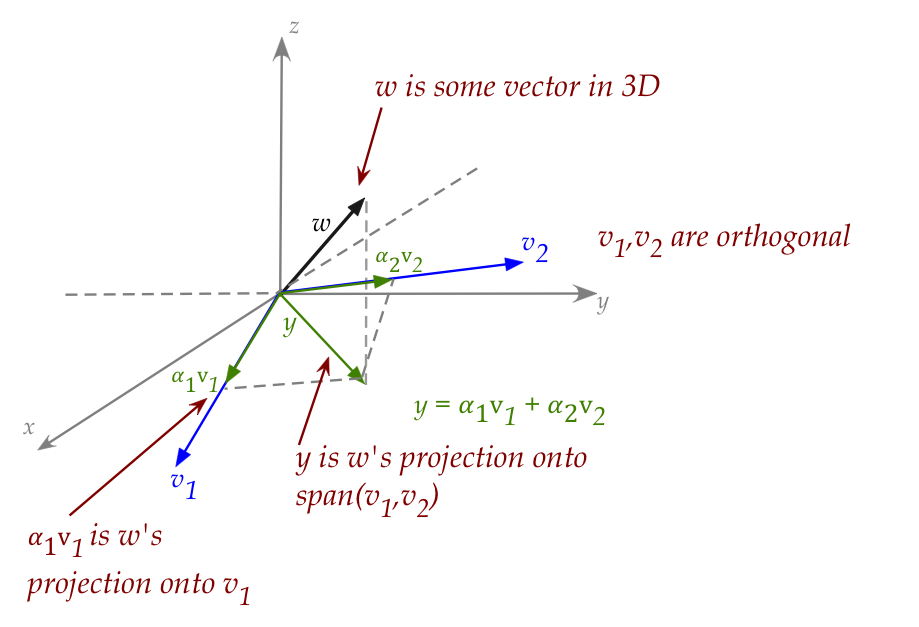
Let's first examine projections with real vectors:
5.2
Projective measurement: what's needed for multiple qubits
Let's start by reviewing, via an example, how projective measurement
worked for the single qubit in some state \(\ksi\):
- Recall, there are four steps:
- Identify the projectors for the measurement basis:
$$
P_{i} \eql \otr{v_i}{v_i}
$$
- Compute each projected vector:
$$
\kt{\psi_{P_i}} \eql P_{i} \ksi
$$
- Compute the squared magnitude of each projection:
$$
\magsq{ \kt{\psi_{P_i}} }
$$
as the probability of seeing the i-th normalized projection
as the outcome.
- Compute each normalized projection (each potential outcome):
$$
\kt{\psi_{N_i}} \eql
\frac{ \kt{\psi_{P_i}} }{ \mag{ \kt{\psi_{P_i}} } }
$$
This gives us each possible outcome and its associated probability:
$$
\mbox{Outcome } \kt{\psi_{N_i}}
\;
\mbox{ occurs with probability } \; \magsq{ \kt{\psi_{P_i}} }
$$
- For example, suppose we measure \(\kt{0}\) in the
basis \(\kt{+}, \kt{-}\).
- This gives us possible outcomes and their associated
probabilities:
$$\eqb{
\mbox{ outcome } & \; \kt{+} \; & \mbox{ occurs with probability } \;
\smf{1}{2} \\
\mbox{ outcome } & \; \kt{-} \; & \mbox{ occurs with probability } \;
\smf{1}{2} \\
}$$
- Now, we could have inferred these directly by examining
the target vector expressed in the measurement basis:
- Express \(\kt{0}\) in the \(\kt{+}, \kt{-}\) basis:
$$
\kt{0} = \isqts{1} \kt{+} + \isqts{1} \kt{-}
$$
- Then, the probability of observing \(\kt{+}\), is just
$$
\magsq{ \isqts{1} } \eql \smf{1}{2}
$$
- Thus, the extra trouble of projective measurement is
often overkill for a single qubit.
Now let's examine projective measurement with two qubits:
- It's here that we run into a complication:
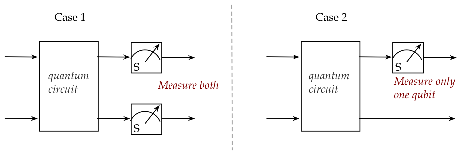
- Are both qubits to be measured together?
- Is it possible to measure just one qubit?
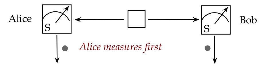
- A second complication: how do we reason about the case
when two qubits are apart?
Let's examine two-qubits-together with an example:
- Consider the two-qubit state
$$
\ksi \eql \isqts{1} \kt{01} + \isqts{1} \kt{10}
$$
- And suppose we use the two-qubit standard basis for
two-qubit measurement:
$$
\kt{00}, \;\;\;\;
\kt{01}, \;\;\;\;
\kt{10}, \;\;\;\;
\kt{11}
$$
- First consider the direct approach:
- The outcomes of measurement are the measurement-basis vectors:
\(\kt{00},\kt{01},\kt{10},\kt{11}\).
- We now express the vector \(\ksi\) in the measurement basis:
$$
\ksi \eql 0\, \kt{00} + \isqts{1} \kt{01} + \isqts{1} \kt{10} + 0
\,\kt{11}
$$
- Thus:
$$\eqb{
\kt{00} & \mbox{ occurs with probability } & 0\\
\kt{01} & \mbox{ occurs with probability } & \magsq{ \isqts{1} }\\
\kt{10} & \mbox{ occurs with probability } & \magsq{ \isqts{1} }\\
\kt{11} & \mbox{ occurs with probability } & 0\\
}$$
- Next, let's see how this works with projective measurement:
- Step 1: Identify the measurement basis projectors:
$$\eqb{
P_{00} & \eql & \otr{00}{00} \\
P_{01} & \eql & \otr{01}{01} \\
P_{10} & \eql & \otr{10}{10} \\
P_{11} & \eql & \otr{11}{11} \\
}$$
- Step 2: Use the above to compute projected vectors:
$$\eqb{
P_{00} \ksi & \eql & \otr{00}{00}
\left( \isqts{1} \kt{01} + \isqts{1} \kt{10} \right)
& \eql & 0 \\
P_{01} \ksi & \eql & \otr{01}{01}
\left( \isqts{1} \kt{01} + \isqts{1} \kt{10} \right)
& \eql & \isqts{1} \kt{01} \\
P_{10} \ksi & \eql & \otr{10}{10}
\left( \isqts{1} \kt{01} + \isqts{1} \kt{10} \right)
& \eql & \isqts{1} \kt{10} \\
P_{11} \ksi & \eql & \otr{11}{11}
\left( \isqts{1} \kt{01} + \isqts{1} \kt{10} \right)
& \eql & 0 \\
}$$
- Step 3: The magnitudes of (non-zero) projected vectors
are their probabilities:
$$\eqb{
\magsq{ P_{01} \ksi } & \eql &
\magsq{ \isqts{1} \kt{01} } & \eql & \smf{1}{2} \\
\magsq{ P_{10} \ksi } & \eql &
\magsq{ \isqts{1} \kt{10} } & \eql & \smf{1}{2} \\
}$$
- Step 4: Normalize the projections to get the outcome vectors:
$$\eqb{
\smf{1}{ \mag{ P_{01} \ksi } } P_{01} \ksi
& \eql & \frac{1}{\isqts{1}} \: \isqts{1} \kt{01}
& \eql & \kt{01} \\
\smf{1}{ \mag{ P_{10} \ksi } } P_{10} \ksi
& \eql & \frac{1}{\isqts{1}} \: \isqts{1} \kt{10}
& \eql & \kt{10} \\
}$$
- Notice the usefulness of Dirac notation in
the second step, for example:
- At this point, projective measurement still seems like overkill.
Now suppose we want to measure only the first qubit:
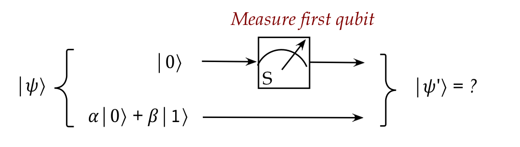
- Suppose the input two-qubit vector is
$$
\ksi \eql \kt{0} \otimes \parenl{ \alpha \kt{0} + \beta\kt{1} }
$$
- We'd like to know: after measuring only the first qubit,
what are the possible states, and with what probabilities?
- Clearly, since the first (top) qubit is already \(\kt{0}\),
measuring this qubit alone should leave the top qubit as \(\kt{0}\).
- Intuition suggests that because there's no entanglement,
the second qubit should be the same.
- That is, after measurement, that state should be
$$
\kt{\psi^\prime} \eql \kt{0} \otimes \parenl{ \alpha \kt{0} + \beta\kt{1} }
$$
- In this case, we can apply tensoring rules to see that
$$
\kt{\psi^\prime} \eql \alpha \parenl{ \kt{0} \otimes \kt{0} }
+ \beta \parenl{ \kt{0} \otimes \kt{1} }
\eql
\alpha \kt{00} + \beta \kt{01}
$$
- Yet, any two-qubit measurement will leave the state either in
\(\kt{00}\) or \(\kt{01}\):
$$
\kt{\psi^\prime} \eql \kt{00}
\;\;\;\;\;\; \mbox{or} \;\;\;\;\;\;
\kt{\psi^\prime} \eql \kt{01}
$$
- Thus, the two types of measurements produce different
results, and we need to extend the theory to account for this.
- Next, consider what happens if the two-qubit state
is entangled:
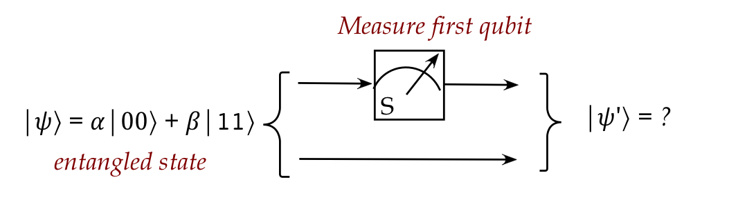
- Here,
$$
\ksi \eql \alpha \kt{00} + \beta\kt{11}
$$
- Intuitively, a first-qubit measurement should
leave the state either in \(\kt{00}\) or \(\kt{11}\)
with probabilities:
$$\eqb{
\mbox{outcome } \kt{00} & \;\; & \mbox{ with probability } \magsq{\alpha}\\
\mbox{outcome } \kt{11} & \;\; & \mbox{ with probability } \magsq{\beta}\\
}$$
- How, then, should we reason about these different scenarios?
- Fortunately, projective measurement is easily extended to
handle these cases.
5.3
Projective measurement: extending the theory to multiple qubits
We want to extend the theory to be able to handle different
measurement scenarios with \(n\) qubits.
Examples of scenarios include:
- Measuring all \(n\) qubits simultaneously.
- Measuring just one qubit amongst the \(n\) qubits.
- Measuring a subset of qubits from the \(n\) qubits.
- And each case, having the freedom to use a variety
of measurement bases.
There are three aspects to extending single-qubit projective
measurement to multiple qubits:
- Understanding how the particular measurement splits
the whole \(n\)-qubit space into orthogonal subspaces.
- Building \(n\)-qubit projectors accordingly.
- Seeing if it helps to construct the
\(n\)-qubit projectors
from smaller projectors (such as 1-qubit projectors).
Let's examine these aspects via a 2-qubit example:
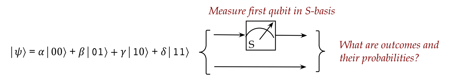
- Here, the input is a general 2-qubit vector
$$
\ksi \eql \alpha \kt{00} + \beta \kt{01} + \gamma \kt{10} +
\delta \kt{11}
$$
- We're measuring the top qubit (left qubit) in the S-basis.
- Clearly, the single-qubit measurement leads to
\(\kt{0}\) or \(\kt{1}\) for that qubit.
- We now ask: what 2-qubit measurement is equivalent
to measuring only the first qubit?
- And, since we want to use projective measurement:
what 2-qubit projector achieves the first-qubit measurement?
- We will go about addressing this question in several stages:
- We'll first examine the potential vectors that result
from subjecting the 2-qubit vector to 1-qubit measurement.
- These potential vectors will form a vector space.
- Then, we'll build the projectors for these spaces.
- We'll also see that the projectors can be built from
tensoring.
- Stage 1: if you measure the first qubit, what
are the possible 2-qubit vectors that result?
- Example: first qubit results in \(\kt{0}\).
- Second qubit could potentially be any state.
- Describe this as the space
$$
V_1 \eql \mbox{span}\setl{ \kt{00}, \kt{01} }
$$
- Any vector in this space has the first qubit as \(\kt{0}\).
- Similarly, the space of 2-qubit vectors that
correspond to "first qubit is \(\kt{1}\)" is
$$
V_2 \eql \mbox{span}\setl{ \kt{10}, \kt{11} }
$$
- Stage 2: Thus, the potential results of first-qubit
measurement lie in two orthogonal subspaces:
$$
V \eql V_1 \cup V_2
$$
where
$$\eqb{
V_1 & \eql & \mbox{span}\setl{ \kt{00}, \kt{01} }
& \mbx{First qubit \(\kt{0}\)} \\
V_2 & \eql & \mbox{span}\setl{ \kt{10}, \kt{11} }
& \mbx{First qubit \(\kt{1}\)} \\
}$$
- Stage 3: Now define projectors for each of these subspaces
$$\eqb{
P_{V_1} & \eql & \otr{00}{00} + \otr{01}{01} \\
P_{V_2} & \eql & \otr{10}{10} + \otr{11}{11} \\
}$$
- Why are these the projectors?
- Recall that a projector for a subspace is the sum
of projectors for basis vectors in that subspace.
- Because \(\kt{00}, \kt{01}\) are orthogonal,
they must constitute a basis for \(\mbox{span}\setl{ \kt{00}, \kt{01} } \).
- Note: applying in Dirac form makes it easy to see why
these are projectors for those subspaces:
- Consider any vector
$$
\ksi \eql \alpha \kt{00} + \beta \kt{01} + \gamma \kt{10} +
\delta \kt{11}
$$
- Then
$$\eqb{
P_{V_1} \ksi & \eql &
\mbox{projection of \(\ksi\) on \(V_1\)} \\
& \eql &
\parenl{ \otr{00}{00} + \otr{01}{01} }
\parenl{ \alpha \kt{00} + \beta \kt{01} + \gamma \kt{10} +
\delta \kt{11} } \\
& \eql &
\alpha \kt{00} + \beta \kt{01} \\
& \eql & \mbox{A vector in } V_1
}$$
Recall: \(V_1 = \mbox{span}\{\kt{00}, \kt{01}\}\)
- Similarly,
$$\eqb{
P_{V_2} \ksi & \eql &
\mbox{projection of \(\ksi\) on \(V_2\)} \\
& \eql &
\gamma \kt{10} + \delta \kt{11} \\
& \eql & \mbox{A vector in } V_2
}$$
- The outcomes of measurement and their probabilities
are
$$\eqb{
\mbox{normalized } P_{V_1} \ksi & \;\; &
\mbox{ occurs with probability } \magsq{ P_{V_1} \ksi } \\
\mbox{normalized } P_{V_2} \ksi & \;\; &
\mbox{ occurs with probability } \magsq{ P_{V_2} \ksi } \\
}$$
- In this case:
- Squared magnitudes of the projections are:
$$\eqb{
\magsq{ P_{V_1} \ksi } & \eql \magsq{ \alpha \kt{00} + \beta \kt{01} }
& \eql & \magsq{\alpha} + \magsq{\beta} \\
\magsq{ P_{V_2} \ksi } & \eql \magsq{ \gamma \kt{10} + \delta \kt{11} }
& \eql & \magsq{\gamma} + \magsq{\delta} \\
}$$
- Normalized projections are:
$$\eqb{
\smf{1}{\mag{ P_{V_1} \ksi }} P_{V_1} \ksi
& \eql & \smf{1}{\sqrt{ \magsq{\alpha} + \magsq{\beta} }}
\parenl{ \alpha \kt{00} + \beta \kt{01} } \\
\smf{1}{\mag{ P_{V_2} \ksi }} P_{V_2} \ksi
& \eql & \smf{1}{\sqrt{ \magsq{\gamma} + \magsq{\delta} }}
\parenl{ \gamma \kt{10} + \delta \kt{11} } \\
}$$
- Let's take a closer look at the first projected
vector to see that it makes sense:
- Recall we started in state
$$
\ksi \eql \alpha \kt{00} + \beta \kt{01} + \gamma \kt{10} +
\delta \kt{11}
$$
- Let's write this as
$$
\ksi \eql \kt{0} \otimes \parenl{ \alpha \kt{0} + \beta \kt{1} }
\;\; + \;\; \kt{1} \otimes \parenl{ \gamma \kt{0} + \delta \kt{1} }
$$
Here, we've just separated out the first qubit for emphasis.
- If we measure the first qubit as \(\kt{0}\), then
the second should be "untouched" in state \(\alpha \kt{0} + \beta \kt{1}\).
- And the resulting 2-qubit vector should be
$$
\kt{0} \otimes \parenl{ \alpha \kt{0} + \beta \kt{1} }
\eql
\alpha \kt{00} + \beta \kt{01}
$$
- But the latter is not normalized, and so, the normalized
vector is:
$$
\smf{1}{\sqrt{ \magsq{\alpha} + \magsq{\beta} }}
\parenl{ \alpha \kt{00} + \beta \kt{01} } \\
$$
Which is what we obtained earlier with the projector-approach.
- Those were the first three stages in understanding
multi-qubit measurement.
- The fourth is about a potential simplification: can
the 2-qubit projectors be built out of smaller 1-qubit projectors?
- Recall that the two 1-qubit S-basis projectors are
$$\eqb{
P_0 & \eql & \otr{0}{0} \\
P_1 & \eql & \otr{1}{1} \\
}$$
- Since we're not measuring the 2nd-qubit, the only projector
that keeps the qubit the same is the identity
$$
I \eql \otr{0}{0} + \otr{1}{1}
$$
(in Dirac form).
- Thus, one can construct the 2-qubit projectors via tensoring
$$\eqb{
P_{V_1} & \eql & P_0 \otimes I & \eql & \otr{0}{0} \otimes
\parenl{ \otr{0}{0} + \otr{1}{1} } \\
P_{V_2} & \eql & P_1 \otimes I & \eql & \otr{1}{1} \otimes
\parenl{ \otr{0}{0} + \otr{1}{1} } \\
}$$
- Let's work out the first one to see the details:
$$\eqb{
P_0 \otimes I & \eql &
\otr{0}{0} \otimes \parenl{ \otr{0}{0} + \otr{1}{1} }
& \mbx{Tensor of projectors} \\
& \eql &
\parenl{ \otr{0}{0} \otimes \otr{0}{0} }
+ \parenl{ \otr{0}{0} \otimes \otr{1}{1} }
& \mbx{Tensor properties}\\
& \eql &
\parenl{ \otr{0 \otimes 0}{0 \otimes 0} }
+ \parenl{ \otr{0 \otimes 1}{0 \otimes 1} }
& \mbx{Proposition 4.5} \\
& \eql &
\otr{00}{00} + \otr{01}{01} & \mbx{Shorthand notation} \\
}$$
Recall the very useful Proposition 4.5 (Module 4):
$$
\otr{v}{v} \otimes \otr{w}{w}
\eql \otr{v \otimes w}{v \otimes w}
$$
- This projector-tensoring is a convenience that, depending on
the particular scenario, may or may not be the fastest way
to solve that scenario.
- Finally, let's remind ourselves of alternative tensoring
notation:
- We can write
$$
\otr{v}{v} \otimes \otr{w}{w}
\eql {\bf \kt{v}\kt{w} \br{v}\br{w} }
\;\;\;\;\;\;\;\;
(\mbox{ Also written as } \otr{v, w}{v, w})
$$
- Thus, we could also have written the earlier projector example as:
$$\eqb{
P_0 \otimes I & \eql &
\otr{0}{0} \otimes \parenl{ \otr{0}{0} + \otr{1}{1} } \\
& \eql &
\parenl{ \otr{0}{0} \otimes \otr{0}{0} }
+ \parenl{ \otr{0}{0} \otimes \otr{1}{1} } \\
& \eql &
\parenl{ \bf \kt{0}\kt{0} \br{0}\br{0} }
+ \parenl{ \bf \kt{0}\kt{1} \br{0}\br{1} }\\
& \eql &
\otr{00}{00} + \otr{01}{01}
}$$
- By convention, we do not write \(\kt{00}\) as \(\kt{0,0}\).
In-Class Exercise 1:
Consider the single-qubit projectors
\(P_+=\otr{+}{+}\) and \(P_- = \otr{-}{-}\).
- Show that \( (P_+ \otimes I)\kt{00} = \isqt{1}\kt{+,0} \)
and \( (P_+ \otimes I)\kt{11} = \isqt{1}\kt{+,1} \)
- Show that \(\isqt{1} \kt{+,0} + \isqt{1} \kt{+,1} = \kt{+,+}\)
- Expand \( (P_+ \otimes I) \) into a matrix and use that
to show \( (P_+ \otimes I) \ksi = \kt{+,+} \) (normalized) where
\(\ksi = \isqt{1}(\kt{00} + \kt{11}) \)
Let's use the results from the exercise above in our next example:
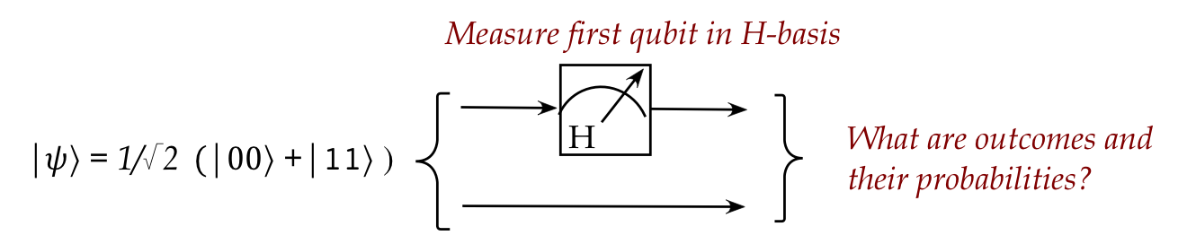
- We wish to measure the first qubit using the H-basis \(\kt{+}, \kt{-}\).
- The input vector is:
$$
\ksi \eql \isqts{1} \parenl{ \kt{00} + \kt{11} }
$$
(Recall: this is the first of the four Bell states.)
- Since the outcomes of the first-qubit measurement are
\(\kt{+}, \kt{-}\), the vector space is split into:
$$\eqb{
V_1 & \eql & \mbox{span}\setl{ \kt{+,0}, \kt{+,1} } \\
V_2 & \eql & \mbox{span}\setl{ \kt{-,0}, \kt{-,1} } \\
}$$
Note:
- We should ask: are \(\kt{+,0}, \kt{+,1}\) orthogonal?
- Yes, because
$$
\inr{+,0}{+,1} \eql \inr{+}{+} \inr{0}{1} \eql 1 \times 0
\eql 0
$$
(The second step follows from how inner products work with tensoring.)
- Aside: the sets \(V_1\) and \(V_2\) can be written with alternative spans, for example:
$$\eqb{
V_1 & \eql & \mbox{span}\setl{ \kt{+,+}, \kt{+,-} } \\
V_2 & \eql & \mbox{span}\setl{ \kt{-,+}, \kt{-,-} } \\
}$$
However, we'll strive to use the standard basis where possible.
- Next, we'll use the constructive approach to build the
projectors \(P_{V_1}, P_{V_2}\) for these subspaces:
$$\eqb{
P_{V_1} & \eql & P_+ \otimes I & \eql & \otr{+}{+} \otimes I \\
P_{V_2} & \eql & P_- \otimes I & \eql & \otr{-}{-} \otimes I \\
}$$
- We might be tempted to work this out in terms of the
standard basis, but let's wait until these projectors "encounter"
the target vector \(\ksi\).
- Now apply the projectors. For example, the above exercise
showed that
$$
P_{V_1} \ksi \eql \isqts{1} \kt{+,+}
$$
Which when normalized is \(\kt{+,+}\).
- Similarly,
$$\eqb{
P_{V_2} \ksi & \eql &
\parenl{ \otr{-}{-} \otimes I } \;\; \isqts{1} \parenl{ \kt{00} + \kt{11} }
& \mbx{Apply projector}\\
& \eql &
\isqts{1}
\parenl{ \otr{-}{-} \otimes I } \parenl{ \kt{0}\otimes\kt{0}
\;\; + \;\; \kt{1}\otimes\kt{1} }
& \mbx{Undo 2-qubit shorthand for clarity}\\
& \eql &
\isqts{1}
\parenl{
\kt{-}\inr{-}{0} \otimes I\kt{0} \;\; + \;\; \kt{-}\inr{-}{1} \otimes I\kt{1}}
& \mbx{Tensor bilinearity and distribution over addition}\\
& \eql &
\smf{1}{2} \parenl{ \kt{-} \otimes \kt{0} \; - \; \kt{-}\otimes\kt{1} }
& \mbx{Apply the 1-qubit operators}\\
& \eql &
\isqts{1} \kt{-} \otimes \isqts{1} \parenl{ \kt{0} - \kt{1} }
& \mbx{Factor out from tensor}\\
& \eql &
\isqts{1} \kt{-} \otimes \kt{-}
& \mbx{Recognize right vector}\\
& \eql &
\isqts{1} \kt{-,-} & \mbx{Shorthand} \\
}$$
(Which will get normalized as\(\kt{-,-}\).)
- Aside: we could have compacted the last few steps
and written it a bit differently as:
$$\eqb{
& \eql &
\smf{1}{2} \parenl{ \kt{-,0} \; - \; \kt{-,1} }\\
& \eql &
\isqts{1} \kt{-} \isqts{1} \parenl{ \kt{0} - \kt{1} }\\
& \eql &
\isqts{1} \kt{-} \kt{-} \\
& \eql &
\isqts{1} \kt{-,-}
}$$
- Thus, the measurement outcomes and probabilities are:
$$\eqb{
\kt{+,+} & \;\;\;\; &
\mbox{ with probability } \smf{1}{2} \\
\kt{-,-} & \;\;\;\; &
\mbox{ with probability } \smf{1}{2} \\
}$$
- Note:
It wasn't obvious that measuring only the first qubit would
result in the second qubit becoming \(\kt{+}\) or \(\kt{-}\).
With these examples, we're now in a position to outline the
theoretical extension of projective measurement to multiple qubits:
- A measurement device corresponds to decomposition of
a multi-qubit vector space \(V\) into a number of orthogonal subspaces:
$$
V \eql V_1 \cup \ldots \cup V_k
$$
- This results in projectors, one per subspace: \(P_{V_i}\).
- Given an input vector \(\ksi \in V\), the possible outcomes
of measurement are normalized versions of
$$
P_{V_1}\ksi, \;\; P_{V_2}\ksi, \;\; \ldots \;\; P_{V_k}\ksi
$$
That is,
$$
\smf{1}{\mag{ P_{V_1}\ksi }} P_{V_1}\ksi, \;\;
\smf{1}{\mag{ P_{V_2}\ksi }} P_{V_2}\ksi, \;\;
\ldots
\smf{1}{\mag{ P_{V_k}\ksi }} P_{V_k}\ksi
$$
- These occur with probabilities
$$\eqb{
\mbox{Outcome } \smf{1}{\mag{ P_{V_1}\ksi }} P_{V_1}\ksi
& \;\;\;\; & \mbox{ with probability } \magsq{ P_{V_1}\ksi } \\
& \vdots & \\
\mbox{Outcome } \smf{1}{\mag{ P_{V_k}\ksi }} P_{V_k}\ksi
& \;\;\;\; & \mbox{ with probability } \magsq{ P_{V_k}\ksi } \\
}$$
- Note:
- We have not proved that this is how measurement
ought to work from some underlying principle.
- In fact, this is a fundamental assumption,
a postulate, of the theory.
In-Class Exercise 2:
Apply the projectors \( (P_+ \otimes I) \)
and \( (P_- \otimes I) \) to
\(\ksi = \frac{1}{2} (\kt{00} + \kt{01} + \kt{10} + \kt{11} \)
using the Dirac-notation approach above, and then confirm
your results by expanding into matrices.
5.4
Projective measurement: examples
Example 1: Let's revisit the E-91 protocol where we left out the
H-basis analysis:
- When both Alice and Bob use the H-basis in sequence,
they see the same single-qubit state:
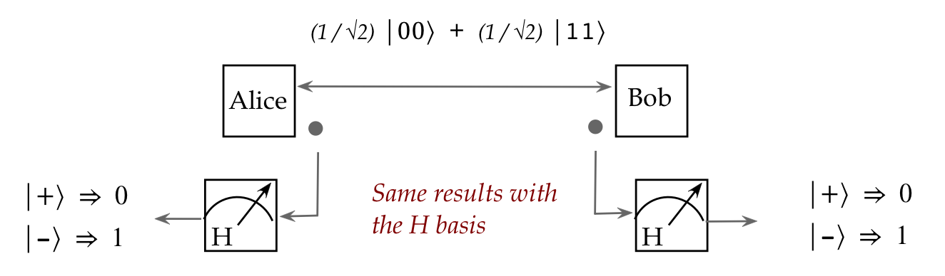
- We already showed that when the S-basis is used in
sequence, the outcomes match for both Alice and Bob.
- With our added theory, we can now show this for the H-basis.
- In the previous section, we showed that a single-qubit
measurement of the entangled (Bell) state
$$
\ksi \eql \isqts{1} \parenl{ \kt{00} + \kt{11} }
$$
with the H-basis resulted in outcomes
$$\eqb{
\kt{+, +} & \;\;\;\; & \mbox{ with probability } \smf{1}{2} \\
\kt{-, -} & \;\;\;\; & \mbox{ with probability } \smf{1}{2} \\
}$$
- These are two outcomes after Alice performs her
single-qubit H-basis measurement.
- Thus, if Alice sees \(\kt{+}\) so will Bob.
- Likewise, if Alice sees \(\kt{-}\) so will Bob.
Thus, their bits match.
Example 2: Consider measurement with the Bell basis:
- Recall the Bell basis:
$$\eqb{
\kt{\Phi^+} & \eql & \isqts{1} \parenl{ \kt{00} + \kt{11} } \\
\kt{\Phi^-} & \eql & \isqts{1} \parenl{ \kt{00} - \kt{11} } \\
\kt{\Psi^+} & \eql & \isqts{1} \parenl{ \kt{01} + \kt{10} } \\
\kt{\Psi^-} & \eql & \isqts{1} \parenl{ \kt{01} - \kt{10} } \\
}$$
This is a 2-qubit basis.
- Suppose we perform a 2-qubit measurement with this basis
on the general 2-qubit vector
$$
\ksi \eql \smf{1}{2}
\parenl{ \alpha\kt{00} + \beta\kt{01} + \gamma\kt{10} +
\delta\kt{11} }
$$
- Since we've said the measurement occurs with this basis,
the four basis vectors are their own subspaces:
$$\eqb{
V_{\Phi^+} & \eql & \mbox{ span}\setl{ \kt{\Phi^+} } \\
V_{\Phi^-} & \eql & \mbox{ span}\setl{ \kt{\Phi^-} } \\
V_{\Psi^+} & \eql & \mbox{ span}\setl{ \kt{\Psi^+} } \\
V_{\Psi^-} & \eql & \mbox{ span}\setl{ \kt{\Psi^-} } \\
}$$
and thus, there are four projectors
$$
\otr{\Phi^+}{\Phi^+},
\;\;\;\;
\otr{\Phi^-}{\Phi^-},
\;\;\;\;
\otr{\Psi^+}{\Psi^+},
\;\;\;\;
\otr{\Psi^-}{\Psi^-},
$$
- Applying the first projector to the input:
$$\eqb{
\parenl{ \otr{\Phi^+}{\Phi^+} } \ksi
& \eql &
\kt{\Phi^+} \inr{\Phi^+}{\psi} \\
& \eql &
\smf{1}{2} \kt{\Phi^+}
\inrh{\Phi^+}{ \alpha\kt{00} + \beta\kt{01} + \gamma\kt{10} +
\delta\kt{11} } \\
& \eql &
\smf{1}{2} \kt{\Phi^+}
\parenl{ \alpha \inr{\Phi^+}{00} + \beta \inr{\Phi^+}{01}
+ \gamma \inr{\Phi^+}{10} + \delta \inr{\Phi^+}{11} } \\
& \eql &
\smf{\alpha + \delta}{2\sqrt{2}} \kt{\Phi^+}
}$$
- Similarly,
$$\eqb{
\parenl{ \otr{\Phi^-}{\Phi^-} } \ksi
& \eql &
\smf{\alpha - \delta}{2\sqrt{2}} \kt{\Phi^-} \\
\parenl{ \otr{\Psi^+}{\Psi^+} } \ksi
& \eql &
\smf{\beta + \gamma}{2\sqrt{2}} \kt{\Psi^+} \\
\parenl{ \otr{\Psi^-}{\Psi^-} } \ksi
& \eql &
\smf{\beta - \gamma}{2\sqrt{2}} \kt{\Psi^-} \\
}$$
- Thus, the outcomes are the Bell vectors with
probabilities
$$\eqb{
\kt{\Phi^+}
& \;\;\;\; & \mbox{ with probability }
\magsq{ \smf{\alpha + \delta}{2\sqrt{2}} } \\
\kt{\Phi^-}
& \;\;\;\; & \mbox{ with probability }
\magsq{ \smf{\alpha - \delta}{2\sqrt{2}} } \\
\kt{\Psi^+}
& \;\;\;\; & \mbox{ with probability }
\magsq{ \smf{\beta + \gamma}{2\sqrt{2}} } \\
\kt{\Psi^-}
& \;\;\;\; & \mbox{ with probability }
\magsq{ \smf{\beta - \gamma}{2\sqrt{2}} }
}$$
- Note:
- This example is merely of theoretical interest.
- Just because we dream up a measurement basis does not mean
it can be physically implemented with an actual device.
Example 3: A hypothetical 3-qubit example:
- Suppose there was a way to test whether two qubits are equal.
- And suppose we apply this to the first and third qubits
of a 3-qubit system.
- Then, such a measurement will divide the space into two subspaces:
$$\eqb{
V_1 & \eql & \mbox{span}\setl{ \kt{000}, \kt{010}, \kt{101},
\kt{111} } \\
V_2 & \eql & \mbox{span}\setl{ \kt{001}, \kt{011}, \kt{100},
\kt{110} } \\
}$$
Note: the vectors spanning \(V_1\) have their first and third bits equal.
- The projectors are:
$$\eqb{
P_{V_1} & \eql &
\otr{000}{000} + \otr{010}{010} + \otr{101}{101} +
\otr{111}{111} \\
P_{V_2} & \eql &
\otr{001}{001} + \otr{011}{011} + \otr{100}{100} +
\otr{110}{110} \\
}$$
- One can then apply these to an input vector \(\ksi\)
in the usual way.
- For example, suppose
$$
\ksi \eql \smf{1}{\sqrt{3}} \parenl{ \kt{000} + \kt{001} +
\kt{010} }
$$
- Then
$$\eqb{
P_{V_1} \ksi
& \eql &
\smf{1}{\sqrt{3}} \parenl{ \kt{000} + \kt{010} } \\
P_{V_2} \ksi
& \eql &
\smf{1}{\sqrt{3}} \kt{001}
}$$
- Thus, the outcomes and probabilities are:
$$\eqb{
\smf{1}{\sqrt{2}} \parenl{ \kt{000} + \kt{010} }
& \;\;\;\;&
\mbox{with probability } \smf{2}{3} \\
\kt{001}
& \;\;\;\;&
\mbox{with probability } \smf{1}{3} \\
}$$
In-Class Exercise 3:
Fill in the missing step of normalization in the above example.
Then, apply the same projectors to the vector \(\ksi=\kt{+,+,+}\)
and list the outcomes and probabilities.
5.5
Projective measurement in stages
Consider measurements in sequence, as in this example:
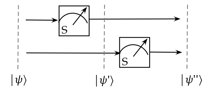
- Here, the input is a 2-qubit state \(\ksi\).
- Then, the top qubit is first measured, which results
in some state \(\kt{\psi^\prime}\).
- After this, the vector is measured in the second qubit,
which leaves the state \(\kt{\psi^{\prime\prime}}\).
- The question arises: is there a single 2-qubit measurement
(for the purpose of further analysis)
that is equivalent to the sequence of 1-qubit measurements?
Let's analyze the above scenario:
- Suppose the input \(\ksi\) is the generic 2-qubit state
$$
\ksi \eql
\parenl{ \alpha\kt{00} + \beta\kt{01} + \gamma\kt{10} +
\delta\kt{11} }
$$
- Now, the projectors for the first measurement are:
$$\eqb{
P_0 & \eql & \otr{0}{0} \otimes I & \eql & \otr{00}{00} + \otr{01}{01} \\
P_1 & \eql & \otr{1}{1} \otimes I & \eql & \otr{10}{10} + \otr{11}{11} \\
}$$
- From which,
$$\eqb{
P_0 \ksi & \eql & \alpha\kt{00} + \beta\kt{01} \\
P_1 \ksi & \eql & \gamma\kt{10} + \delta\kt{11}
}$$
which we'll normalize and name:
$$\eqb{
\kt{\psi_0} & \eql &
\smf{1}{ \mag{ P_0 \ksi } }
P_0 \ksi & \eql & \smf{1}{\sqrt{|\alpha|^2 + |\beta|^2 } }
\parenl{ \alpha\kt{00} + \beta\kt{01} }\\
\kt{\psi_1} & \eql &
\smf{1}{ \mag{ P_1 \ksi } }
P_1 \ksi & \eql & \smf{1}{\sqrt{|\gamma|^2 + |\delta|^2 } }
\parenl{ \gamma\kt{10} + \delta\kt{11} }
}$$
- Next, each of these outcomes occur with the following
probabilities:
$$\eqb{
\kt{\psi_0} & \;\;\;\; &
\mbox{occurs with probability }
\magsq{ P_0 \ksi } & \eql & \magsq{\alpha} + \magsq{\beta} \\
\kt{\psi_1} & \;\;\;\; &
\mbox{occurs with probability }
\magsq{ P_1 \ksi } & \eql & \magsq{\gamma} + \magsq{\delta} \\
}$$
- Now for a given measurement, either one (but not both) will
be an input into the second measurement.
- We'll consider both cases.
- The projectors for the second measurement are:
$$\eqb{
P_2 & \eql & I \otimes \otr{0}{0}
& \eql & \otr{00}{00} + \otr{10}{10} \\
P_3 & \eql & I \otimes \otr{1}{1}
& \eql & \otr{01}{01} + \otr{11}{11} \\
}$$
- We will next apply these projectors to the possible
outcomes, \(\kt{\psi_0}\) and \(\kt{\psi_1}\), from the first stage:
$$\eqb{
P_2 \kt{\psi_0} & \eql &
\parenl{ \otr{00}{00} + \otr{10}{10} }
\smf{1}{\sqrt{|\alpha|^2 + |\beta|^2 } }
\parenl{ \alpha\kt{00} + \beta\kt{01} }
& \eql & \smf{\alpha}{\sqrt{|\alpha|^2 + |\beta|^2 } } \kt{00} \\
P_2 \kt{\psi_1} & \eql &
\parenl{ \otr{00}{00} + \otr{10}{10} }
\smf{1}{\sqrt{|\gamma|^2 + |\delta|^2 } }
\parenl{ \gamma\kt{10} + \delta\kt{11} }
& \eql & \smf{\gamma}{\sqrt{|\gamma|^2 + |\delta|^2 } } \kt{10} \\
P_3 \kt{\psi_0} & \eql &
\parenl{ \otr{01}{01} + \otr{11}{11} }
\smf{1}{\sqrt{|\alpha|^2 + |\beta|^2 } }
\parenl{ \alpha\kt{00} + \beta\kt{01} }
& \eql & \smf{\beta}{\sqrt{|\alpha|^2 + |\beta|^2 } } \kt{01} \\
P_3 \kt{\psi_1} & \eql &
\parenl{ \otr{01}{01} + \otr{11}{11} }
\smf{1}{\sqrt{|\gamma|^2 + |\delta|^2 } }
\parenl{ \gamma\kt{10} + \delta\kt{11} }
& \eql & \smf{\delta}{\sqrt{|\gamma|^2 + |\delta|^2 } } \kt{11} \\
}$$
- Observe that the outcomes (normalized)
are the standard 2-qubit vectors:
\(\kt{00}, \kt{01}, \kt{10}, \kt{11}\).
- These occur with probabilities
$$\eqb{
\kt{00} & \;\;\;\; &
\mbox{occurs with probability } \magsq{\alpha} \\
\kt{01} & \;\;\;\; &
\mbox{occurs with probability } \magsq{\beta} \\
\kt{10} & \;\;\;\; &
\mbox{occurs with probability } \magsq{\gamma} \\
\kt{11} & \;\;\;\; &
\mbox{occurs with probability } \magsq{\delta} \\
}$$
(See exercise below to fill in one step: how
did terms like \(\sqrt{|\alpha|^2 + |\beta|^2}\)
and \(\sqrt{|\gamma|^2 + |\delta|^2}\) disappear?)
- But these are exactly the outcomes and probabilities
one gets with 2-qubit measurement in the standard basis!
- That is, with projectors
$$\eqb{
Q_0 & \eql & \otr{00}{00} \\
Q_1 & \eql & \otr{01}{01} \\
Q_2 & \eql & \otr{10}{10} \\
Q_3 & \eql & \otr{11}{11} \\
}$$
applied to
$$
\ksi \eql
\alpha\kt{00} + \beta\kt{01} + \gamma\kt{10} +
\delta\kt{11}
$$
one gets the same outcomes with the same probabilities.
- Thus, we've answered the question: what 2-qubit
measurement corresponds to the sequence of 1-qubit measurements from earlier?
In-Class Exercise 4:
There was one step missing in the sequence of projections above:
what happened to the terms
\(\sqrt{|\alpha|^2 + |\beta|^2}\) and \(\sqrt{|\gamma|^2 + |\delta|^2}\)?
Hint: write down the probabilities
\(\magsq{ P_0\ksi }\) and \(\magsq{ P_2\kt{\psi_0} }\),
and then ask: what product of probabilities leads us to
observing \(\kt{00}\) as the outcome?
Combining projectors in sequenced measurements:
- We went through a lot of trouble in applying the two sets
of projectors in sequence above.
- Let's ask: could we have applied the projectors in sequence
and then normalized?
- The answer is: yes!
(And the algebra is much simpler.)
- Recall that we started with input vector \(\ksi\).
- Then we applied the first stage:
$$\eqb{
P_0 \ksi & \eql & \parenl{ \otr{0}{0} \otimes I } \ksi \\
P_1 \ksi & \eql & \parenl{ \otr{1}{1} \otimes I } \ksi
}$$
- Now consider applying the second stage directly, without
normalizing:
$$\eqb{
P_2 P_0 \ksi & \eql &
\parenl{ I \otimes \otr{0}{0} }
\parenl{ \otr{0}{0} \otimes I } \ksi \\
P_2 P_1 \ksi & \eql &
\parenl{ I \otimes \otr{0}{0} }
\parenl{ \otr{1}{1} \otimes I } \ksi \\
P_3 P_0 \ksi & \eql &
\parenl{ I \otimes \otr{1}{1} }
\parenl{ \otr{0}{0} \otimes I } \ksi \\
P_3 P_1 \ksi & \eql &
\parenl{ I \otimes \otr{1}{1} }
\parenl{ \otr{1}{1} \otimes I } \ksi \\
}$$
- Now use the rules for tensors of matrices:
\((A \otimes B)(C \otimes D) = (AC \otimes BD)\).
- Applying, we see that
$$\eqb{
P_2 P_0 \ksi & \eql &
\parenl{ \otr{0}{0} \otimes \otr{0}{0} } \ksi
& \eql &
\otr{00}{00} \ksi \\
P_2 P_1 \ksi & \eql &
\parenl{ \otr{1}{1} \otimes \otr{0}{0} } \ksi
& \eql &
\otr{10}{10} \ksi \\
P_3 P_0 \ksi & \eql &
\parenl{ \otr{0}{0} \otimes \otr{1}{1} } \ksi
& \eql &
\otr{01}{01} \ksi \\
P_3 P_1 \ksi & \eql &
\parenl{ \otr{1}{1} \otimes \otr{1}{1} } \ksi
& \eql &
\otr{11}{11} \ksi \\
}$$
These are just the standard-basis 2-qubit projectors.
- Thus, we see that the theory we developed earlier for
tensoring projectors is useful:
\(\rhd\)
It's best to combine projectors and simplify.
There is an important practical implication:
- Physically implementing a 2-qubit measurement is difficult.
- What we've seen is that a 2-qubit standard-basis measurement
can be done in two stages of standard-basis 1-qubit measurements.
- This is what happens in practice.
5.6
Unitary actions in sequence and across qubits
We of course want to "do things" to qubits before measuring.
The only way to change qubits without measuring is to apply
a unitary operation.
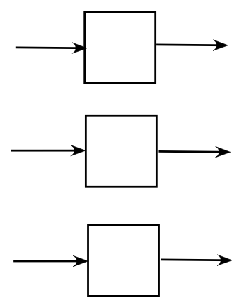
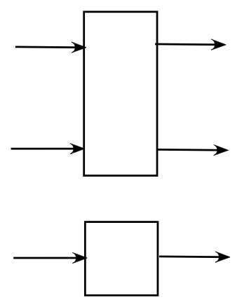
Let's highlight a few general aspects to applying unitary operations:
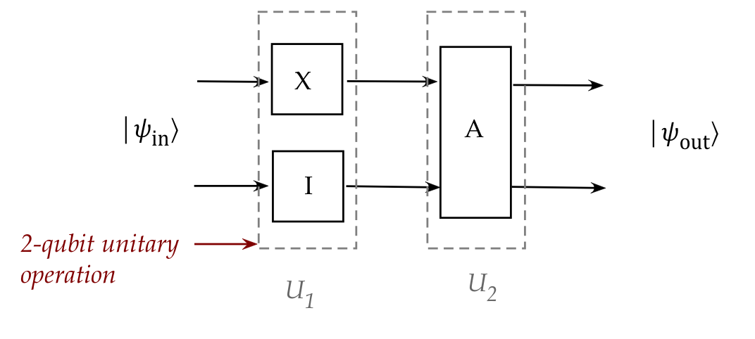
- Consider this 2-qubit example:
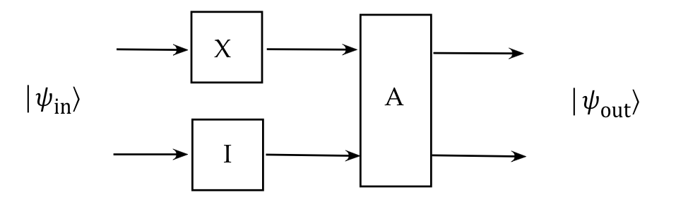
- \(X\) and \(I\) are 1-qubit unitary operators.
- \(A\) is a 2-qubit operator.
- We want to know: what is the output vector as a result
of applying these operators to the input vector?
- Our diagramming uses the "flying qubit" paradigm to imagine
a multi-qubit vector going from left to right through the unitary operators.
- Thus, we will be interested in the multi-qubit state at each
stage:
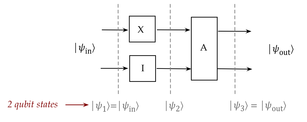
- Think of the dashed lines representing stages in the
time-evolution of this system.
- Thus, initial 2-qubit state is \(\kt{\psi_1}\).
- After the application of \(X\) to the first qubit, and no
change \(I\) to the second, the 2-qubit state is now \(\kt{\psi_2}\).
- We've seen that this corresponds to the unitary operator
$$
X \otimes I \eql \mat{0 & 1\\ 1 & 0} \otimes I
\eql \mat{0 & I\\ I & 0}
\eql \mat{0 & 0 & 1 & 0\\
0 & 0 & 0 & 1\\
1 & 0 & 0 & 0\\
0 & 1 & 0 & 0}
$$
- After applying the operator \(A\) the result is \(\kt{\psi_3}\).
- Here, we're going to use
$$
A
\eql \mat{0 & 0 & 0 & 1\\
0 & 0 & 1 & 0\\
0 & 1 & 0 & 0\\
1 & 0 & 0 & 0}
$$
- At every stage a complete 2-qubit unitary operation applies:
- Even though nothing is done to the second qubit, we
write that as the "do nothing" operator \(I\).
- We could (and will often) draw:
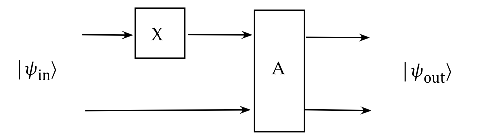
- But this obscures the fact that the first stage
is really the 2-qubit operator \(X \otimes I\).
- These aspects become more clear algebraically:
- Suppose the input 2-qubit vector is \(\ksi\).
- The first stage produces
$$
\kt{\psi_2} \eql (X \otimes I) \ksi
$$
- And this is acted on by the second stage:
$$
\kt{\psi_3} \eql A \kt{\psi_2}
$$
- Which we can combine as:
$$
\kt{\psi_3} \eql A (X \otimes I) \ksi
$$
- Let's emphasize the matrix dimensions:
$$
\kt{\psi_3}_{4\times 1} \eql A_{4\times 4}
\parenl{ X_{2\times 2} \otimes I_{2\times 2} } \ksi_{4\times 1}
$$
Thus, we could not write
$$\eqb{
\kt{\psi_3} \eql A X \ksi & \mbx{Incorrect!}
}$$
In-Class Exercise 5:
- Show that \(X^2=I\) both with matrix and Dirac forms.
- Write out the matrix and Dirac forms of \(X \otimes X\).
Continuing with the example:
- Suppose the operator \(A\) happens to be \(A = X\otimes X\).
- Then the two stages can be tensored as:
$$\eqb{
A (X \otimes I)
& \eql &
(X \otimes X)(X \otimes I)
& \mbx{Sub for \(A\)} \\
& \eql & (XX \otimes XI)
& \mbx{Tensor bilinearity}\\
& \eql & (I \otimes X)
& \mbx{Shown in exercise}\\
}$$
- Now let's apply this to the generic 2-qubit vector
$$
\ksi \eql \alpha\kt{00} + \beta\kt{01}
+ \gamma\kt{10} + \delta \kt{11}
$$
- In Dirac form
$$\eqb{
I \otimes X
& \eql &
\parenl{ \otr{0}{0} + \otr{1}{1} }
\otimes
\parenl{ \otr{0}{1} + \otr{1}{0} }
& \mbx{Dirac versions of the 1-qubit ops} \\
& \eql &
\parenl{ \otr{0}{0} \otimes \otr{0}{1} }
+ \parenl{ \otr{0}{0} \otimes \otr{1}{0} }
+ \parenl{ \otr{1}{1} \otimes \otr{0}{1} }
+ \parenl{ \otr{1}{1} \otimes \otr{1}{0} }
& \mbx{Distribution over +} \\
& \eql &
\otr{00}{01} + \otr{01}{00} + \otr{10}{11} + \otr{11}{10}
& \mbx{Tensor rules for outer-products} \\
}$$
- Thus,
$$\eqb{
\parenl{ I \otimes X } \ksi
& \eql &
\parenl{ \otr{00}{01} + \otr{01}{00} + \otr{10}{11} +
\otr{11}{10} }
\alpha\kt{00} + \beta\kt{01}
+ \gamma\kt{10} + \delta \kt{11} \\
& \eql &
\beta\kt{00} + \alpha\kt{01}
+ \delta\kt{10} + \gamma \kt{11} \\
}$$
In-Class Exercise 6:
Confirm the above result with the matrix form of
\((I \otimes X) \ksi\).
Let's now generalize these ideas to the n-qubit case:
- A single-qubit unitary operation \(A_k\) performed on the k-th qubit
corresponds to the n-qubit unitary operation
$$
I \otimes I \otimes \ldots \otimes A_k \otimes \ldots
\otimes I
$$
- When a sequence of n-qubit operations are applied:
- The diagram goes left to right.
- But the matrices go right to left:
$$
U_m U_{m-1} \ldots U_2 U_1 \ksi
$$
- That is, \(U_1\) is first applied, then \(U_2\) etc.
- A collection of multi-qubit operators can be applied
at any stage, for example:
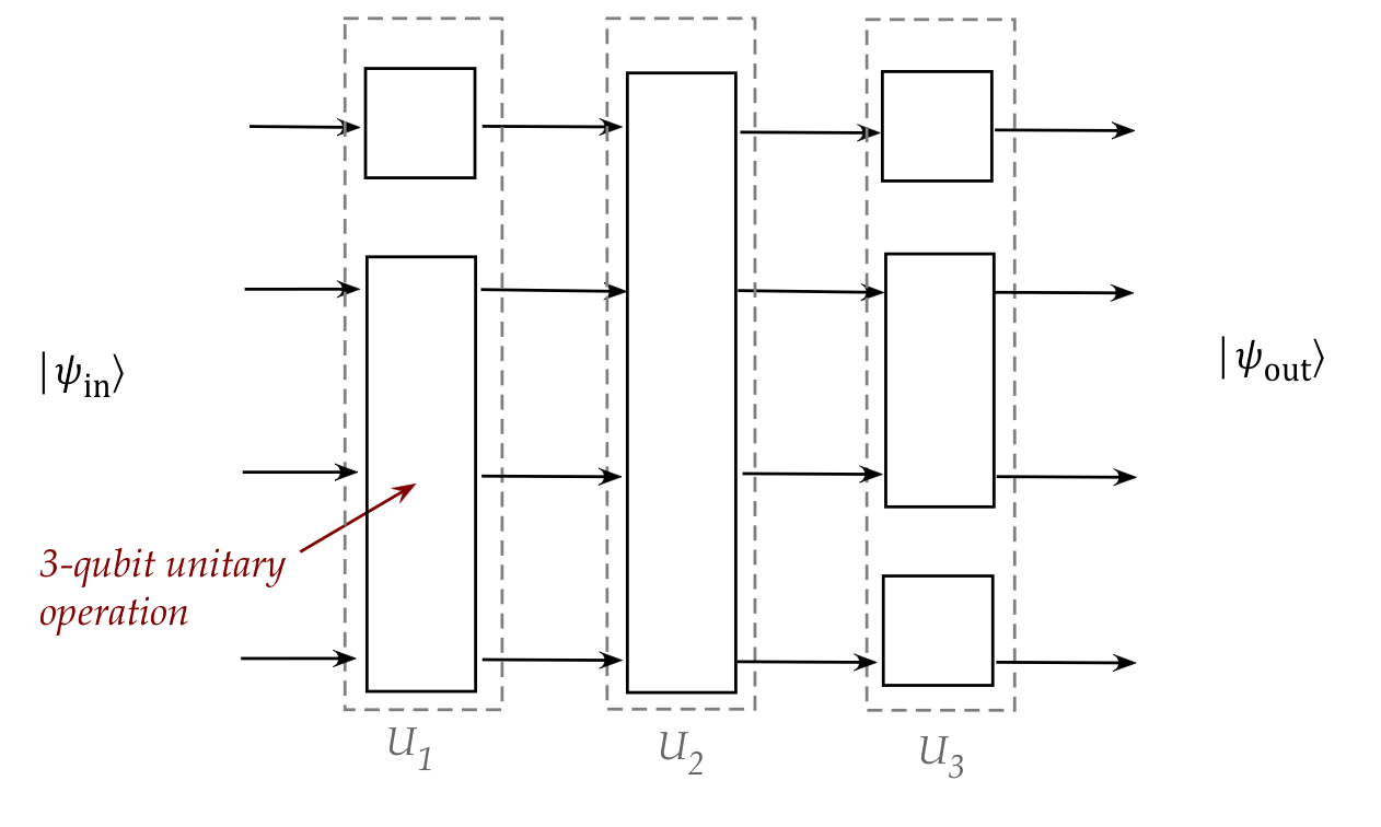
Here:
- Think of tensoring applying vertically.
- The first stage, for example, is a tensor of 1-qubit unitary with
a 3-qubit unitary.
- And regular operator products applied horizontally:
\(U_m U_{m-1} \ldots U_2 U_1\)
- The theory developed earlier showed that:
- Tensored unitary operators (going vertically)
are unitary.
- Products of unitary operators (going horizontally)
are unitary.
- The big implication:
- Quantum computations can be created by designing
unitary operations in sequence, each of which is
composed (vertically) of smaller operations.
- Where does measurement fit in?
- The answer: anywhere!
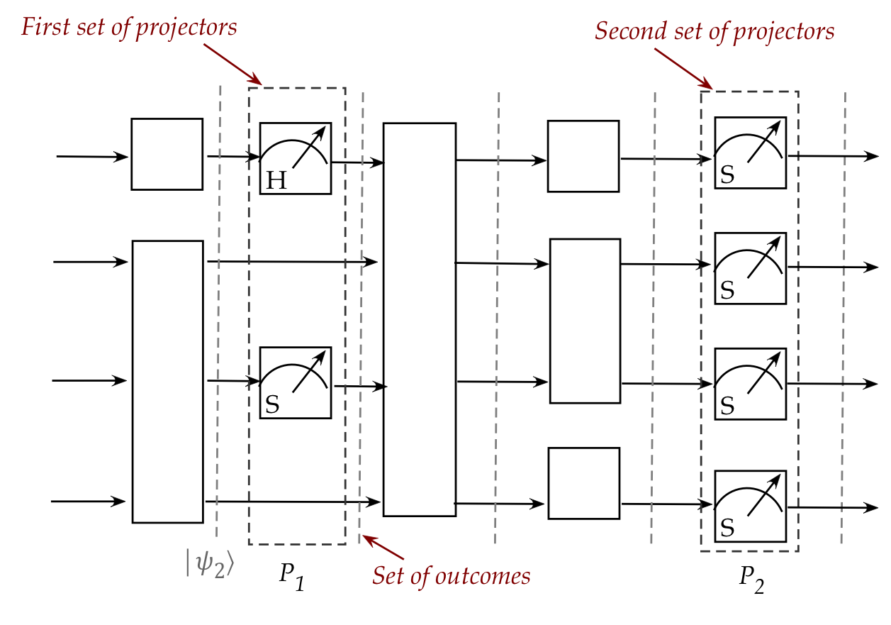
- When a measurement occurs, it is represented by a
set of projectors (for each basis vector of the measuring device).
\(\rhd\)
We cannot apply a single projector.
- After the first measurement, the outcomes are probabilistic
and cannot be represented by a single state.
- Typically, all measurements occur after
the last unitary operation:
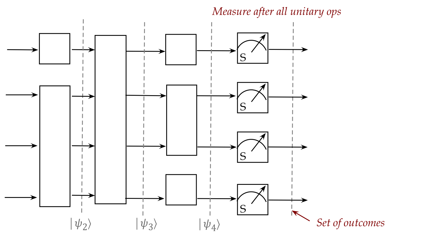
- This is easier to analyze.
- The basis is most often the standard basis.
- This unitary-followed-by-measurement is called the
standard ciruit model.
The task of developing a quantum computation is now clear
in this framework:
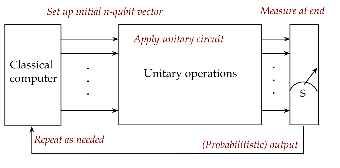
- Figure out the unitary operations and assemble them into a circuit.
- Analyse the results of measurement to infer the
outcomes.
- Repeat as needed.
What remains for us:
- What unitary operations are useful (and practical to implement)?
- How does one systematically construct a circuit?
- How do circuits lead to useful algorithms?
- How can we exploit quantum parallelism?
Let's explore the last point:
- You might have noticed a problem with the classical-quantum
looped architecture above:
- If a classical computer sets up an initial n-qubit vector
like \(\kt{00\ldots 0}\), why not just have the classical
computer simulate the circuit?
- The advantage: no randomness!
- However, consider this 2-qubit input state:
$$
\ksi \eql \smf{1}{2} \parenl{ \kt{00} + \kt{01} + \kt{10} +
\kt{11} }
$$
Note:
- All four 2-qubit basis vectors are "in there".
- We might hope that a circuit acting on \(\ksi\) somehow
does something to each basis vector at the same time.
- For 3 qubits, the equivalent state that combines all
basis vectors with equal weight is:
$$
\ksi \eql \smf{1}{\sqrt{8}}
\parenl{ \kt{000} + \kt{001} + \kt{010} + \kt{011}
+ \kt{100} + \kt{101} + \kt{110} + \kt{111} }
$$
If measured, the probability of seeing any one of them is the same:
\(\left( \frac{1}{\sqrt{8}} \right)^2 = \frac{1}{8}\)
- We can extend this to n-qubits with the state:
$$
\ksi \eql \smf{1}{\sqrt{2^n}}
\parenl{ \kt{00\ldots 0} + \ldots + \kt{11\ldots 1} }
$$
- Terminology: superposition
- The term superposition simply refers to a linear combination.
- The above examples are sometimes called equal-superposition
states for the standard basis.
- An equal-superposition state is often the starting state
for many quantum algorithms.
- The potential for speed up or parallelism:
- If a circuit acts on the equal-superposition state,
it can act on all \(2^n\) states at the same time.
- This has the potential of providing exponential speed
up over classical machines.
- However, measurement can "ruin" this potential because the
outcomes are probabilistic, and because it forces the state
into one of the \(2^n\) basis vectors.
- Precisely explaining quantum speed-up remains an unresolved issue:
- Some results show that entanglement must be present when
speed-up occurs.
- Other results show speed up without exploiting superposition.
5.7
The Hadamard operator
The Hadamard operator is one of the most important
operators in quantum computing:
- It is frequently used to create the n-qubit equal-superposition
as the input vector for a computation.
- It also features in intermediate computations, sometimes
just on one qubit.
To see where it comes from,
we'll start with the 1-qubit idea of transforming \(\kt{0}\) into
the 1-qubit equal-superposition
$$
\kt{+} \eql \isqts{1} \kt{0} + \isqts{1} \kt{1}
$$
- Suppose there is some unitary operator \(H\) such that
$$
H \kt{0} \eql \isqts{1} \kt{0} + \isqts{1} \kt{1}
$$
- In matrix form, this unknown operator could be represented
by four numbers
$$
\mat{a & b\\ c & d}
\mat{1\\ 0}
\eql
\isqts{1} \kt{0} + \isqts{1} \kt{1}
$$
or
$$
\mat{a\\ c} \eql \mat{ \isqt{1} \\ \isqt{1}}
$$
- Since the rows are orthonormal, we must have
$$\eqb{
\magsq{a} + \magsq{b} & \eql & 1 \\
\magsq{c} + \magsq{d} & \eql & 1 \\
}$$
or
$$\eqb{
\magsq{b} & \eql & 1 - \magsq{a} & \eql & 1 - \left( \isqts{1}
\right) & \eql & \frac{1}{2} \\
\magsq{d} & \eql & 1 - \magsq{c} & \eql & 1 - \left( \isqts{1}
\right) & \eql & \frac{1}{2} \\
}$$
- Thus,
$$\eqb{
b & \eql & \pm \isqts{1} \\
d & \eql & \pm \isqts{1} \\
}$$
However:
- \(b\) and \(d\) cannot have the same sign.
- For example
$$
\mat{ \isqt{1} & \isqt{1} \\ \isqt{1} & \isqt{1} }
$$
would not work because the two columns are not orthogonal.
- But either of
$$
\mat{ \isqt{1} & \isqt{1} \\ \isqt{1} & -\isqt{1} }
\;\;\;\;\;\;\;\;
\mbox{ or }
\;\;\;\;\;\;\;\;
\mat{ \isqt{1} & -\isqt{1} \\ \isqt{1} & \isqt{1} }
$$
would work.
- The former is the \(H\) operator
and gives us the definition of \(\kt{-}\):
$$
H \kt{1} \eql
\mat{ \isqt{1} & \isqt{1} \\ \isqt{1} & -\isqt{1} }
\mat{0\\ 1}
\eql
\mat{ \isqt{1}\\ -\isqt{1}}
\eql \kt{-}
$$
- Thus, in the 1-qubit case, the Hadamard operator \(H\)
creates equal-superposition:
$$
H \kt{0} \eql \isqts{1} \kt{0} + \isqts{1} \kt{1}
$$
- Terminology: \(H\) is also called the Walsh-Hadamard transform.
Next consider equal superposition in 2 qubits:
- The vector in this case is:
$$
\ksi \eql
\smf{1}{2} \kt{00}
+ \smf{1}{2} \kt{01}
+ \smf{1}{2} \kt{10}
+ \smf{1}{2} \kt{11}
$$
- We now seek a 2-qubit unitary operator to transform
\(\kt{00}\) into \(\ksi\):
$$
A \kt{00} \eql \smf{1}{2} \kt{00}
+ \smf{1}{2} \kt{01}
+ \smf{1}{2} \kt{10}
+ \smf{1}{2} \kt{11}
$$
- Observe that
$$\eqb{
\kt{+}\kt{+}
& \eql &
\kt{+} \otimes \kt{+} \\
& \eql &
\isqts{1} (\kt{0} + \kt{1}) \; \otimes \; \isqts{1} (\kt{0} + \kt{1}) \\
& \eql &
\smf{1}{2} \kt{00}
+ \smf{1}{2} \kt{01}
+ \smf{1}{2} \kt{10}
+ \smf{1}{2} \kt{11}
}$$
- So, clearly the desired operator \(A\) will satisfy
$$
A \kt{00} \eql \kt{+} \otimes \kt{+}
$$
or
$$
A (\kt{0} \otimes \kt{0}) \eql \kt{+} \otimes \kt{+}
$$
- But we showed in the 1-qubit case that \(H\kt{0} = \kt{+}\).
- Substituting,
$$
\kt{+} \otimes \kt{+}
\eql
H\kt{0} \otimes H\kt{0}
\eql
\parenl{ H \otimes H } \parenl{ \kt{0} \otimes \kt{0} }
$$
which means we've found our operator
$$
A \eql H \otimes H
$$
- And because tensor products preserve unitarity,
\(H \otimes H\) is unitary.
The n-qubit version:
- The n-qubit equal-superposition merely tensors \(\kt{+}\) qubits:
$$\eqb{
& & \hspace{-20pt}
\kt{+}\kt{+}\ldots\kt{+} \\
& \eql &
\parenl{ \isqts{1} \kt{0} + \isqts{1} \kt{1} }
\otimes
\parenl{ \isqts{1} \kt{0} + \isqts{1} \kt{1} }
\otimes \ldots \otimes
\parenl{ \isqts{1} \kt{0} + \isqts{1} \kt{1} } \\
& \eql &
\left( \isqts{1} \right)^n
\parenl{ \kt{00\ldots 0} + \kt{00\ldots 1} + \ldots + \kt{11\ldots 1} }
}$$
- Which means the transform needed to convert \(\kt{00\ldots
0}\) into this vector is:
$$
H \otimes H \otimes \ldots \otimes H \; \defn \; H^{\otimes n}
$$
- Thus we write
$$
H^{\otimes n} \kt{00\ldots 0} \eql
\smf{1}{\sqrt{2^n}}
\parenl{ \kt{00\ldots 0} + \kt{00\ldots 1} + \ldots + \kt{11\ldots 1} }
$$
- It's often convenient to pull out the number \(\frac{1}{\sqrt{2^n}}\)
in matrix form, as in:
$$
H \eql \smf{1}{\sqrt{2}}
\mat{1 & 1\\ 1 & -1}
$$
leaving the matrix itself with only \(1\) or \(-1\) as entries.
- From this, we can easily separate out into the
1-qubit projectors and write
$$\eqb{
H & \eql & \smf{1}{\sqrt{2}}
\left(
\mat{1 & 0\\ 0 & 0}
+ \mat{0 & 1\\ 0 & 0}
+ \mat{0 & 0\\ 1 & 0}
- \mat{0 & 0\\ 0 & 1}
\right) \\
& \eql & \smf{1}{\sqrt{2}}
\parenl{ \otr{0}{0} + \otr{0}{1} + \otr{1}{0} - \otr{1}{1} }
}$$
The Dirac form, as we've seen, is useful in some cases.
In-Class Exercise 7:
Write down the matrices for \(H^{\otimes 2}\) and \(H^{\otimes 3}\)
in the above form (pulling out \(\frac{1}{\sqrt{2^n}}\)).
This is admittedly a bit tedious but will be useful when
we analyze the structure of this matrix for algorithmic insight.
5.8
The \(\cnot\) operator
The \(\cnot\) operator is our first example of a 2-qubit
operator that cannot be expressed as a tensor
of 1-qubit operators.
That is, it is not possible to find 1-qubit operators \(A\)
and \(B\) such that
$$
\cnot \eql A \otimes B
$$
(We showed this in Module 4: see the solved problems).
Let's take a closer look:
- \(\cnot\) = Controlled-NOT.
- In matrix form:
$$
\cnot \eql
\begin{array}{c c}
& \begin{array}{c c c c}{\scriptsize 00} & {\scriptsize 01} &
{\scriptsize 10} & {\scriptsize 11} \\ \end{array} \\
\begin{array}{c c c c}
{\scriptsize 00}\\ {\scriptsize 01}\\ {\scriptsize 10}\\
{\scriptsize 11}
\end{array} &
\left[
\begin{array}{c c c c}
1 & 0 & 0 & 0 \\
0 & 1 & 0 & 0 \\
0 & 0 & 0 & {\bf 1} \\
0 & 0 & 1 & 0 \\
\end{array}
\right]
\end{array}
$$
where we have labeled the rows and columns.
- By examining the \(1\)'s above, we can write this in Dirac
outer-product form as:
$$
\cnot \eql
\otr{00}{00} + \otr{01}{01}
+ {\bf \otr{10}{11}} + \otr{11}{10}
$$
Notice: the term \(\otr{10}{11}\) signifies a \(1\) in
row \(10\) and column \(11\).
- From this, we can easily see what \(\cnot\) does
to the four standard basis vectors:
$$\eqb{
\cnot \kt{00} & \eql & \kt{00} \\
\cnot \kt{01} & \eql & \kt{01} \\
\cnot \kt{10} & \eql & \kt{11} \\
\cnot \kt{11} & \eql & \kt{10} \\
}$$
- An intuitive description is:
- If the first qubit is \(\kt{0}\) leave the second qubit as
is.
- If the first qubit is \(\kt{1}\) flip the second qubit.
Thus, the first qubit serves as a "control" on what happens to the second.
- We now have the first hint of an "if-then" type of operator.
- One can also see this when writing
$$
\cnot \eql \otr{0}{0} \otimes I \; + \; \otr{1}{1} \otimes X
$$
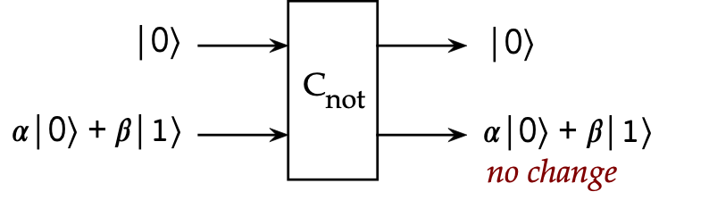
- Let's apply this to: control in the first,
general qubit in the second:
- Let
$$
\ksi \eql \kt{0} \otimes (\alpha\kt{0} + \beta\kt{1})
$$
Then,
$$\eqb{
\cnot \ksi & \eql &
\parenl{ \otr{0}{0} \otimes I + \otr{1}{1} \otimes X }
\parenl{ \kt{0} \otimes \alpha\kt{0} + \beta\kt{1} } \\
& \eql &
\parenl{ \otr{0}{0} \otimes I}
\parenl{ \kt{0} \otimes \alpha\kt{0} + \beta\kt{1} } \\
& &
\plss
\parenl{ \otr{1}{1} \otimes X }
\parenl{ \kt{0} \otimes \alpha\kt{0} + \beta\kt{1} } \\
& \eql &
\kt{0}\inr{0}{0} \otimes I (\alpha\kt{0} + \beta\kt{1})
\plss
\kt{1} \inr{1}{0} \otimes X (\alpha\kt{0} + \beta\kt{1}) \\
& \eql &
\kt{0} \otimes (\alpha\kt{0} + \beta\kt{1})
}$$
Which we can draw as:
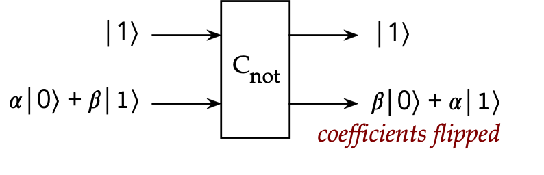
- Now let
$$
\kt{\psi^\prime} \eql \kt{1} \otimes (\alpha\kt{0} + \beta\kt{1})
$$
Then,
$$\eqb{
\cnot \kt{\psi^\prime} & \eql &
\parenl{ \otr{0}{0} \otimes I + \otr{1}{1} \otimes X }
\parenl{ \kt{1} \otimes \alpha\kt{0} + \beta\kt{1} } \\
& \eql &
\kt{1} \otimes (\beta\kt{0} + \alpha\kt{1})
}$$
which flips the coefficients on the second qubit.
In a figure:
- That \(\cnot\) is unitary can be seen from the matrix:
- Every 1 in the matrix does not share its row and column with
another 1.
\(\rhd\)
Rows and columns are orthogonal.
- Each row/column has unit length.
-
Such a matrix is also called a permutation matrix
because multiplying it into a vector permutes its components
as in:
$$
\mat{1 & 0 & 0 & 0\\
0 & 1 & 0 & 0\\
0 & 0 & 0 & 1\\
0 & 0 & 1 & 0}
\mat{a\\ b\\ c\\ d}
\eql
\mat{a\\ b\\ d\\ c}
$$
- About permutation matrices:
- They are unitary.
- If \(P\) is a permutation matrix, \(P^T\) un-does the permutation.
\(\rhd\)
That is, \(P^{-1} = P^T\).
- Another way of saying this: \(P^\dagger = P^T\)
- This property will be useful when constructing quantum circuits.
- \(\cnot\) is Hermitian:
$$
\cnot^\dagger \eql \cnot
$$
And because it's also unitary
$$
\cnot^{-1} \eql \cnot^\dagger \eql \cnot
$$
In-Class Exercise 8:
- Use the Dirac form to apply \(\cnot\) to
\(\ksi= (\alpha\kt{0} + \beta\kt{1}) \otimes \kt{0}\)
and
\(\kt{\psi^\prime} = (\alpha\kt{0} + \beta\kt{1}) \otimes \kt{1}\).
- Then confirm with matrix versions.
- Apply this to the case where \(\alpha=\beta=\isqt{1}\).
Superposition in the control bit:
- We see something more interesting when we send a superposition
as the control bit:
- First, with the target bit as \(\kt{0}\):
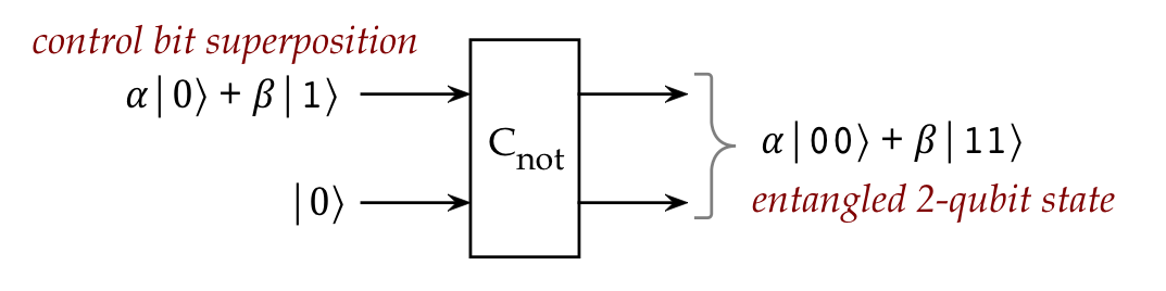
- Then, with \(\kt{1}\):
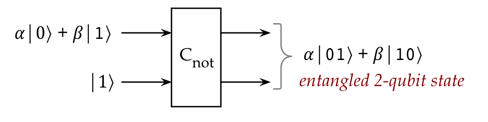
- Thus, the \(\cnot\) operator can entangle two qubits.
- In particular, we can now create Bell states,
for example with \(\alpha = \beta = \isqt{1}\):
$$
\cnot \parenl{ \isqts{1}(\kt{0} + \kt{1}) \otimes \kt{0} }
\eql \isqts{1} (\kt{00} + \kt{11})
\eql \kt{\Phi^+}
$$
or, more compactly,
$$
\kt{\Phi^+} \eql \cnot \kt{+,0}
$$
- Recall that \(\cnot\) is its own inverse, which means
$$
\cnot \kt{\Phi^+} \eql \kt{+,0} \eql \kt{+} \otimes \kt{0}
$$
That is, \(\cnot\) can disentangle some entangled states.
In-Class Exercise 9:
Use the above ideas to draw a two-stage circuit that takes the
vector \(\kt{00}\) to \(\kt{\Phi^+}\)
\(\cnot\) and Hadamard basis vectors:
- Let's apply \(\cnot\) to \(\kt{+}\kt{+}\):
$$\eqb{
\cnot \kt{+}\kt{+}
& \eql &
\parenl{ \otr{0}{0} \otimes I \; + \; \otr{1}{1} \otimes X}
\parenl{ \kt{+} \otimes \kt{+} } \\
& \eql &
\parenl{ \otr{0}{0} \otimes I } \: \parenl{ \kt{+} \otimes \kt{+} }
\;\; + \;\;
\parenl{ \otr{1}{1} \otimes X } \: \parenl{ \kt{+} \otimes \kt{+} } \\
& \eql &
\otr{0}{0} \kt{+} \otimes I\kt{+}
\; + \; \otr{1}{1} \kt{+} \otimes X\kt{+} \\
& \eql &
\isqts{1} \kt{0} \otimes \kt{+}
\; + \; \isqts{1} \kt{1} \otimes \kt{+} \\
& \eql &
\parenl{ \isqts{1} (\kt{0} + \kt{1}) } \otimes \kt{+} \\
& \eql &
\kt{+,+}
}$$
- The effect of \(\cnot\) on the 2-qubit Hadamard basis
vectors:
$$\eqb{
\cnot \kt{+, +} & \eql & \kt{+,+}
& \mbx{First unchanged when second is \(\kt{+}\)} \\
\cnot \kt{-, +} & \eql & \kt{-,+}
& \mbx{Same} \\
\cnot \kt{+, -} & \eql & \kt{-,-}
& \mbx{First flips when second is \(\kt{-}\)} \\
\cnot \kt{-, -} & \eql & \kt{+,-}
& \mbx{Same as above} \\
}$$
(See exercise below.)
- We now see that, without intending so, the second
qubit is the "control" qubit with the Hadamard vectors.
- What to make of this?
- One has to be careful in assigning intuition to quantum operations.
- It is not correct to say that (with S-basis) the first
bit controls the result of the second.
- Instead, it's better to think of a operator's result as
specific to vectors of interest.
- And then, one separately analyzes what happens with other vectors.
Thus, in designing a quantum circuit, one must be acutely aware
of what inputs the circuit will see, and what the output will be.
In-Class Exercise 10:
Show the steps in applying \(\cnot\) to each of:
\(\kt{-,+}, \kt{+,-}, \kt{-,-}\).
Back to the standard basis, and some notation:
- There is a convenient notation one uses with the standard basis.
- Recall the 2-qubit standard basis:
$$
\kt{00},
\;\;\;\;\;\;\;\;
\kt{01},
\;\;\;\;\;\;\;\;
\kt{10},
\;\;\;\;\;\;\;\;
\kt{11}
$$
- One can read the binary digits inside as
$$\eqb{
\kt{b_1b_0} & \eql & \kt{00}
& \mbx{When \(b_1=0, b_0=0\)} \\
\kt{b_1b_0} & \eql & \kt{01}
& \mbx{When \(b_1=0, b_0=1\)} \\
\kt{b_1b_0} & \eql & \kt{10}
& \mbx{When \(b_1=1, b_0=0\)} \\
\kt{b_1b_0} & \eql & \kt{11}
& \mbx{When \(b_1=1, b_1=0\)} \\
}$$
Here,
- \(b_0\) is the binary digit in the \(0\)-th (or \(2^0\))
positional location.
- Likewise, \(b_1\) is the value in the \(2^1\) position.
- The actual numeric value is: \(b_1 2^1 + b_0 2^0\).
- Thus, one can write the set of standard basis vectors as:
$$
\mbox{2-qubit S-basis} \eql
\setl{\kt{b_1b_0}: b_i \in \{0,1\} }
$$
-
This is probably excessive for the simple 2-qubit basis, but will
be useful when we consider the general n-qubit basis:
$$
\mbox{n-qubit S-basis} \eql
\setl{\kt{b_{n-1}\ldots b_1b_0}: b_i \in \{0,1\} }
$$
- The decimal version or numeric value of the binary number is:
$$
b_{n-1} 2^{n-1} + \ldots + b_1 2^1 + b_0 2^0
\eql
\sum_{i=0}^{n-1} b_i 2^i
$$
Note:
the indexing begins with \(0\), reflecting the appropriate power
of 2.
- Where clarity is needed, commas will be used to separate
the binary digits, as in:
$$\eqb{
\kt{b_1, b_0} & \eql & \kt{b_1, b_0}\\
\kt{01} & \eql & \kt{0, 1}
}$$
- Recall (from the Review), the
XOR binary digit operator:
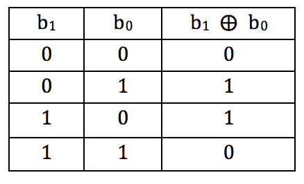
- XOR is a operator that acts on two binary digits
(bits) to produce a bit.
- One way to describe XOR is that one bit (control) flips
the other if the control=1.
- Then, one can write the effect of \(\cnot\)
on the S-basis vectors as:
$$
\cnot \kt{b_1, b_0} \eql \kt{b_1, b_1\oplus b_0}
$$
- To see why, let's write out the four cases:
$$\eqb{
\cnot \kt{00} & \eql & \kt{0, 0 \oplus 0} & \eql & \kt{00}\\
\cnot \kt{01} & \eql & \kt{0, 0 \oplus 1} & \eql & \kt{01}\\
\cnot \kt{10} & \eql & \kt{1, 1 \oplus 0} & \eql & \kt{11}\\
\cnot \kt{11} & \eql & \kt{1, 1 \oplus 1} & \eql & \kt{10}\\
}$$
- Note:
- We have introduced a way to tie Boolean logic to quantum states.
- This will become important as we start to develop quantum circuits.
Lastly, let's show how \(\cnot\) can be derived from its
S-basis transformation:
- Recall that an operator can be described through its
effect on a basis:
- Suppose \(A\) is an operator and \(\kt{v_1},\ldots,\kt{v_n}\)
is a basis
- The operator \(A\) is fully specified if one knows
\(A\kt{v_i}\) for every basis vector \(\kt{v_i}\).
- Then, one can derive the matrix form using the sandwich
approach (Module 2):
$$
A_{ij} \eql \swich{v_i}{A}{v_j}
$$
- Let's see this approach at work with \(\cnot\).
- That is, our starting point is the desired transformation
$$\eqb{
\cnot \kt{00} & \eql & \kt{00} \\
\cnot \kt{01} & \eql & \kt{01} \\
\cnot \kt{10} & \eql & \kt{11} \\
\cnot \kt{11} & \eql & \kt{10} \\
}$$
- Now build the matrix:
$$
\cnot \eql
\mat{
\swich{00}{\cnot}{00} & \swich{00}{\cnot}{01} & \swich{00}{\cnot}{10}
& \swich{00}{\cnot}{11} \\
\swich{01}{\cnot}{00} & \swich{01}{\cnot}{01} & \swich{01}{\cnot}{10}
& \swich{01}{\cnot}{11} \\
\swich{10}{\cnot}{00} & \swich{10}{\cnot}{01} & \swich{10}{\cnot}{10}
& \swich{10}{\cnot}{11} \\
\swich{11}{\cnot}{00} & \swich{11}{\cnot}{01} & {\bf \swich{11}{\cnot}{10}}
& \swich{11}{\cnot}{11} \\
}
$$
Which gives us
$$
\cnot \eql
\mat{1 & 0 & 0 & 0\\
0 & 1 & 0 & 0\\
0 & 0 & 0 & 1\\
0 & 0 & {\bf 1} & 0}
$$
For example, the bolded entry is:
$$
\swich{11}{\cnot}{10} \eql \inr{11}{11} \eql 1
$$
- This approach can be used to derive other operators, but
one would still need to make sure that the result is unitary.
- For example, suppose we want to derive an operator \(A\) that does
this:
$$\eqb{
A \kt{00} & \eql & \kt{01} \\
A \kt{01} & \eql & \kt{00} \\
A \kt{10} & \eql & \kt{10} \\
A \kt{11} & \eql & \kt{11} \\
}$$
That is, when the first qubit is \(\kt{0}\), flip the second.
- Applying the "sandwich" approach:
$$
A \eql
\mat{
\swich{00}{A}{00} & \bf{ \swich{00}{A}{01}} & \swich{00}{A}{10}
& \swich{00}{A}{11} \\
\swich{01}{A}{00} & \swich{01}{A}{01} & \swich{01}{A}{10}
& \swich{01}{A}{11} \\
\swich{10}{A}{00} & \swich{10}{A}{01} & \swich{10}{A}{10}
& \swich{10}{A}{11} \\
\swich{11}{A}{00} & \swich{11}{A}{01} & \swich{11}{A}{10}
& \swich{11}{A}{11} \\
}
\eql
\mat{
0 & {\bf 1} & 0 & 0 \\
1 & 0 & 0 & 0 \\
0 & 0 & 1 & 0 \\
0 & 0 & 0 & 1 \\
}
$$
where, for example, because \(A\kt{01}=\kt{00}\), we have
$$
\swich{00}{A}{01} \eql \inr{00}{00} \eql 1
$$
- Observe that \(A\) is unitary and that
$$
A \eql \otr{0}{0} \otimes X \; + \; \otr{1}{1} \otimes I,
$$
which matches intuition.
- One can describe the effect of \(A\) on
standard basis vectors more compactly as
$$
A \kt{b_1, b_0} \eql \kt{b_1, (b_1\oplus b_0)^\prime}
$$
5.9
3-qubit examples
Let's now look at some examples of applying three tensored 1-qubit
operators to three qubits:
- Example: changing one qubit
$$\eqb{
& & \hspace{-20pt}
(I \otimes X \otimes I) \;
\isqts{1} \parenl{ \kt{000} + \kt{111} } \\
& \eql &
\isqts{1} (I \otimes X \otimes I)
\parenl{ \kt{0}\otimes \kt{0}\otimes \kt{0} \;\; + \;\;
\kt{1}\otimes \kt{1}\otimes \kt{1} } \\
& \eql &
\isqts{1}
\parenl{ I\kt{0}\otimes X\kt{0}\otimes I\kt{0} \;\; + \;\;
I\kt{1}\otimes X\kt{1}\otimes I\kt{1} } \\
& \eql &
\isqts{1}
\parenl{ \kt{0}\otimes \kt{1}\otimes \kt{0} \;\; + \;\;
\kt{1}\otimes \kt{0}\otimes \kt{1} } \\
& \eql &
\isqts{1}
\parenl{ \kt{010}+ \kt{101} }
}$$
- Example: changing one qubit
$$\eqb{
& & \hspace{-20pt}
(H \otimes I \otimes I) \kt{000}\\
& \eql &
H\kt{0} \otimes \kt{0} \otimes \kt{0} \\
& \eql &
\isqts{1} \parenl{\kt{0} + \kt{1} } \otimes \kt{0} \otimes \kt{0} \\
& \eql &
\isqts{1} \parenl{\kt{0}\kt{0}\kt{0} + \kt{1}\kt{0}\kt{0} }\\
& \eql &
\isqts{1} \parenl{\kt{000} + \kt{100} }\\
}$$
- Example: changing one qubit
$$\eqb{
& & \hspace{-20pt}
(I \otimes I \otimes iY) \parenl{ \kt{11} \otimes (\alpha\kt{1} -
\beta\kt{0}) } \\
& \eql &
(I \otimes I \otimes iY)
\parenl{ \kt{1} \otimes \kt{1} \otimes (\alpha\kt{1} - \beta\kt{0}) }\\
& \eql &
I\kt{1} \otimes I\kt{1} \otimes iY(\alpha\kt{1} - \beta\kt{0}) \\
& \eql &
\kt{1} \otimes \kt{1} \otimes (\alpha\kt{0} + \beta\kt{1}) \\
& \eql &
\alpha \kt{110} + \beta\kt{111}
}$$
where \(Y\) is the Pauli operator
$$
Y \eql \mat{0 & -i\\ i & 0}
$$
and so
$$
iY (\alpha\kt{1} - \beta\kt{0})
\eql
\mat{0 & 1\\ -1 & 0} \mat{-\beta\\ \alpha}
\eql
\mat{\alpha \\ \beta}
\eql \alpha\kt{0} + \beta\kt{1}
$$
- Example: Changing two qubits
$$\eqb{
& & \hspace{-20pt}
(I \otimes X \otimes Z)
\isqts{1} \parenl{ \kt{000} + \kt{111} } \\
& \eql &
\isqts{1}
\parenl{ I\kt{0}\otimes X\kt{0}\otimes Z\kt{0} \;\; + \;\;
I\kt{1}\otimes X\kt{1}\otimes Z\kt{1} } \\
& \eql &
\isqts{1}
\parenl{ \kt{0}\otimes \kt{1}\otimes \kt{0} \;\; + \;\;
\kt{1}\otimes \kt{0}\otimes -\kt{1} } \\
& \eql &
\isqts{1}
\parenl{ \kt{010} - \kt{101} }
}$$
Recall the 1-qubit Pauli operator \(Z\):
$$
Z (\alpha\kt{0} + \beta\kt{1})
\eql \alpha\kt{0} - \beta\kt{1}
$$
In-Class Exercise 11:
- Show that
$$\eqb{
& \; &
(H \otimes I \otimes I)
\isqts{1} \parenl{ \alpha\kt{000} + \alpha\kt{011}
+ \beta\kt{110} + \beta\kt{101} }\\
& \eql &
\smf{1}{2}
\parenl{
\kt{00} \otimes (\alpha\kt{0} + \beta\kt{1})
\plss
\kt{01} \otimes (\beta\kt{0} + \alpha\kt{1})
\plss
\kt{10} \otimes (\alpha\kt{0} - \beta\kt{1})
\plss
\kt{11} \otimes (\alpha\kt{1} - \beta\kt{0})
}
}$$
Hint: see one of the solved problems
- Show that
$$
(I \otimes I \otimes Z) (\kt{10} \otimes (\alpha\kt{0} - \beta\kt{1}))
\eql
\kt{10} (\alpha\kt{0} + \beta\kt{1})
$$
One can also apply a 2-qubit operator on two of three qubits,
with a 1-qubit operator on the remaining:
- For example:
$$\eqb{
& & \hspace{-20pt}
(\cnot \otimes I) \parenl{ \isqts{1} \kt{000} + \isqts{1}
\kt{111} } \\
& \eql &
\isqts{1} (\cnot \otimes I) \parenl{ \kt{00}\kt{0} + \kt{11}\kt{1} }\\
& \eql &
\isqts{1} \parenl{ \cnot\kt{00} \otimes I\kt{0}
+ \cnot\kt{11}\otimes I\kt{1} }\\
& \eql &
\isqts{1} \parenl{ \kt{00} \otimes \kt{0}
+ \kt{10}\otimes \kt{1} }\\
& \eql &
\isqts{1} \parenl{ \kt{000} + \kt{101} }
}$$
- Another example that will shortly be useful:
$$\eqb{
& & \hspace{-20pt}
(\cnot \otimes I) \isqts{1}
\parenl{ \alpha \kt{000} + \alpha\kt{011}
+ \beta\kt{101} + \beta \kt{111} } \\
& \eql &
\isqts{1}
\parenl{ \alpha \cnot\kt{00}\kt{0} + \alpha\cnot\kt{01}\kt{1}
+ \beta\cnot\kt{10}\kt{1} + \beta\cnot\kt{11}\kt{1} }\\
& \eql &
\isqts{1}
\parenl{ \alpha \kt{00}\kt{0} + \alpha\kt{01}\kt{1}
+ \beta\kt{11}\kt{1} + \beta\kt{10}\kt{1} }\\
& \eql &
\isqts{1}
\parenl{ \alpha \kt{000} + \alpha\kt{011}
+ \beta\kt{111} + \beta\kt{101} }\\
}$$
5.10
The no-cloning theorem
Consider the possibility of a unitary operator that
copies or clones:
- Suppose \(U\) is such an operator:
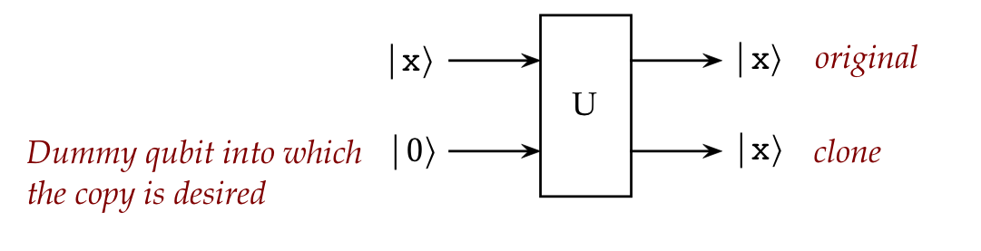
- The target is the top qubit \(\kt{x}\)
- We need a qubit (second one) into which the copy is made.
- The destination qubit has to be in some state.
\(\rhd\)
For now, let's assume that state is \(\kt{0}\)
- Since \(U\) should work for any qubit state,
it must be true that:
$$\eqb{
U \parenl{ \kt{x} \otimes \kt{0} } \eql \kt{x} \otimes \kt{x} \\
U \parenl{ \kt{y} \otimes \kt{0} } \eql \kt{y} \otimes \kt{y} \\
}$$
- To get used to an alternative, more compact notation for
tensored vectors, let's write this as:
$$\eqb{
U \parenl{ \kt{x} \kt{0} } \eql \kt{x} \kt{x} \\
U \parenl{ \kt{y} \kt{0} } \eql \kt{y} \kt{y} \\
}$$
- Let
$$
\ksi \eql \isqts{1} ( \kt{x} + \kt{y} )
$$
- Then, \(U\) should clone this too:
$$
U \parenl{ \ksi \kt{0} } \eql \ksi \ksi
$$
- The right side when simplified becomes
$$\eqb{
\ksi \ksi
& \eql &
\isqts{1} ( \kt{x} + \kt{y} )
\otimes
\isqts{1} ( \kt{x} + \kt{y} ) \\
& \eql &
\smf{1}{2} \parenl{
\kt{x} \kt{x}
+ \kt{x} \kt{y}
+ \kt{y} \kt{x}
+ \kt{y} \kt{y}
}
}$$
- Meanwhile, with the left side
$$\eqb{
U \parenl{\ksi \kt{0}}
& \eql &
U \parenl{\isqts{1} ( \kt{x} + \kt{y} ) \kt{0}} \\
& \eql &
U \parenl{\isqts{1} (\kt{x} \kt{0}) + (\kt{y} \kt{0})} \\
& \eql &
\isqts{1} U (\kt{x} \kt{0}) + \isqts{1} U(\kt{y}\kt{0}) \\
& \eql &
\isqts{1} (\kt{x} \kt{x}) + \isqts{1} (\kt{y} \kt{y})
}$$
- Thus, the two sides are not equal:
$$
\smf{1}{2} \parenl{
\kt{x} \kt{x}
+ \kt{x} \kt{y}
+ \kt{y} \kt{x}
+ \kt{y} \kt{y}
}
\; \neq \;
\isqts{1} \parenl{ \kt{x} \kt{x} + \kt{y} \kt{y} }
$$
- This shows that no unitary cloning operator exists
that will work on all qubit states.
- One minor issue: did the above proof rely on the
second qubit's initial state being \(\kt{0}\)?
- No, \(\kt{0}\) just makes it easier to read.
- The exact same proof would work with any initial state:
$$\eqb{
U \parenl{ \kt{x} \kt{v} } \eql \kt{x} \kt{x} \\
U \parenl{ \kt{y} \kt{v} } \eql \kt{y} \kt{y} \\
}$$
- Note: there are particular states and operators
for which cloning does work, for example:
$$\eqb{
\cnot \kt{00} & \eql & \kt{00}\\
\cnot \kt{10} & \eql & \kt{11}\\
}$$
Here, the first qubit state gets copied into the second.
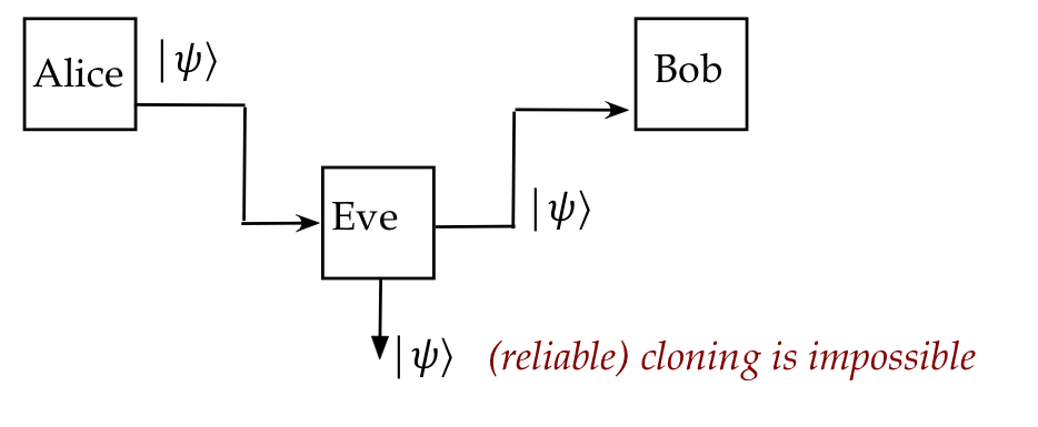
- What's important to keep in mind:
- The goal of cloning is to reliably copy an unknown quantum
state without measuring it.
(Any measurement of course can destroy the state.)
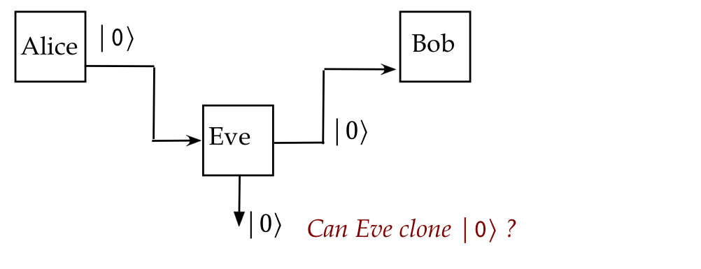
Let's revisit the BB-84 protocol:
- Recall: Alice and Bob use either the S or H bases:
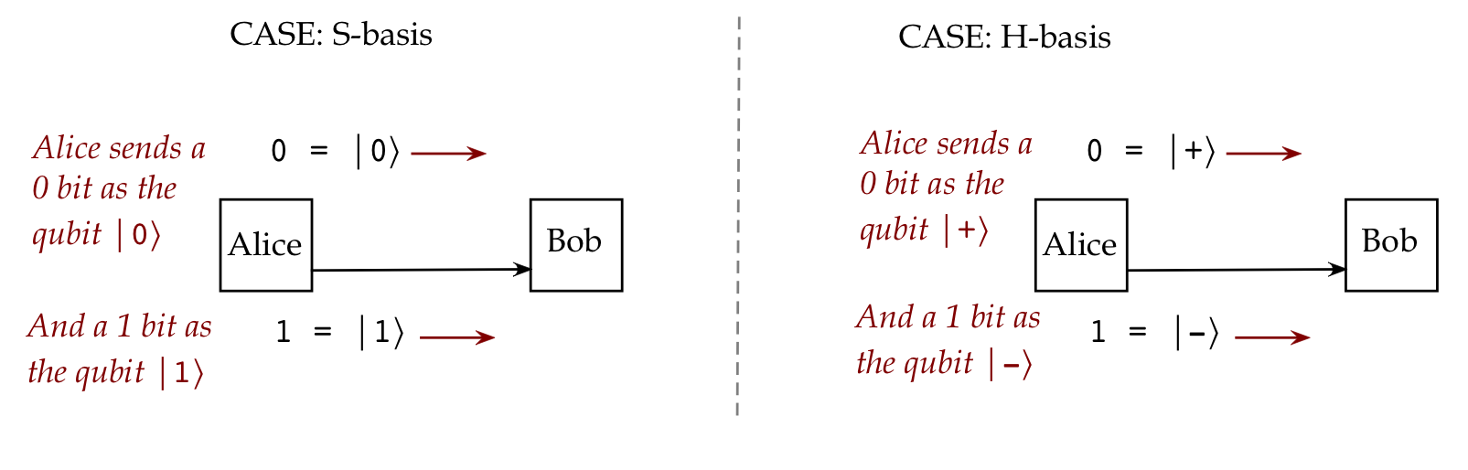
- The security relied on Eve's inability to clone:
- However, Eve knows the protocol: she only needs an operator
to clone four states: \(\kt{0}, \kt{1}, \kt{+}, \kt{-}\).
- For example:
- Now, there's good and bad news. Let's start with the good.
- Consider again a supposed unitary operator that clones:
$$\eqb{
U \parenl{ \kt{x} \kt{0} } \eql \kt{x} \kt{x} \\
U \parenl{ \kt{y} \kt{0} } \eql \kt{y} \kt{y} \\
}$$
- The inner product of the two right sides is:
$$\eqb{
\parenl{ \kt{x} \kt{x} }^\dagger \parenl{ \kt{y} \kt{y} }
& \eql &
\inrh{ \br{x} \br{x} }{ \kt{y} \kt{y} } \\
& \eql &
\inr{x}{y} \inr{x}{y} \\
& \eql &
\inr{x}{y}^2
}$$
- The inner-product of the two left sides:
$$\eqb{
\parenl{ U (\kt{x} \kt{0}) }^\dagger
\parenl{ U (\kt{y} \kt{0}) }
& \eql &
\parenl{ \br{x}\br{0} } U^\dagger U \parenl{ \kt{y}\kt{0} } \\
& \eql &
\parenl{ \br{x}\br{0} } \parenl{ \kt{y}\kt{0} } \\
& \eql &
\inr{x}{y} \inr{0}{0} \\
& \eql &
\inr{x}{y} \\
}$$
- Both inner products must be equal and so
$$
\inr{x}{y} \eql \inr{x}{y}^2
$$
- This is true only if \(\inr{x}{y}=0\) or \(\inr{x}{y}=1\).
- Thus, if the two vectors are not orthogonal, exact
cloning of both is not possible.
- This is certainly the case with BB-84's use of \(\kt{0}\)
and \(\kt{+}\).
- However, the Buzek-Hillery algorithm shows that it is
possible to clone randomly with a reasonably high chance of success:
- They use a 3rd qubit as a "helper" qubit and design a
3-qubit unitary \(U\) such that:
$$\eqb{
U\kt{0}\kt{0}\kt{0}
& \eql &
\sqrt{ \smf{2}{3} } \kt{0}\kt{0}\kt{0}
+ \sqrt{ \smf{1}{6} } \kt{0}\kt{1}\kt{1}
+ \sqrt{ \smf{1}{6} } \kt{1}\kt{0}\kt{1} \\
U\kt{1}\kt{0}\kt{0}
& \eql &
\sqrt{ \smf{2}{3} } \kt{1}\kt{1}\kt{1}
+ \sqrt{ \smf{1}{6} } \kt{1}\kt{0}\kt{0}
+ \sqrt{ \smf{1}{6} } \kt{0}\kt{1}\kt{0} \\
}$$
- This achieves cloning of the first qubit with probability
\(\frac{2}{3}\) if the state is \(\kt{0}\) or \(\kt{1}\).
- Then, they show that any state in the first qubit
can be cloned in the same way with \(U\):
$$
U\kt{\psi}\kt{0}\kt{0}
\eql
\sqrt{ \smf{2}{3} } \kt{\psi}\kt{\psi}\kt{\psi}
+ \sqrt{ \smf{1}{6} } \kt{\psi}\kt{\psi^\perp}\kt{\psi^\perp}
+ \sqrt{ \smf{1}{6} } \kt{\psi^\perp}\kt{\psi}\kt{\psi^\perp}
$$
- The implication for BB-84?
- Alice and Bob may need more bits to see whether Eve is
tampering.
- Or BB-84 may need to be enhanced in other ways.
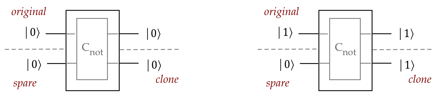
A special and useful case of cloning:
- While a cloning operator does not exist that will work
for general vectors, one can reliably clone special vectors.
- For example, \(\cnot\) gates can be used to clone
standard-basis vectors.
- We already know this for a single standard-basis qubit state:
- This can be extended to cloning any n-qubit standard basis
vector, for example:
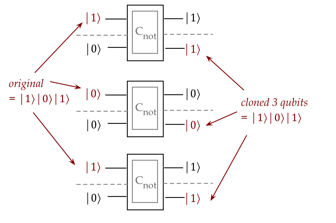
- Note: the cloning is designed specifically for
\(\kt{0}\) as the "spare" qubit.
(It doesn't work if the "spare" was \(\kt{1}\).)
5.11
Quantum teleportation
While perfect cloning is not possible, a transfer
of an unknown quantum state is possible, even across large distances.
This transfer is known as quantum teleportation.
It does not achieve cloning because the original state is destroyed.
And it needs the "help" of additional classical bits.
We'll now outline the steps:
- Step 1: Alice has a qubit in some unknown state \(\ksi\).
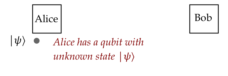
The goal is for Alice to have this state transferred to Bob.
- Let's write the unknown state as:
$$
\ksi \eql \alpha\kt{0} + \beta\kt{1}
$$
- Step 2: Alice and Bob get one qubit each from an
entangled Bell state:
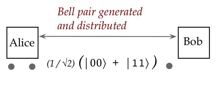
Here, we're using the first Bell state:
$$
\kt{\Phi^+} \eql \isqts{1} \parenl{ \kt{00} + \kt{11} }
$$
- Thus, the three qubits are in state
$$\eqb{
\kt{T} & \eql & \ksi \otimes \kt{\Phi^+} \\
& \eql &
\parenl{ \alpha\kt{0} + \beta\kt{1} }
\otimes
\isqts{1} \parenl{ \kt{00} + \kt{11} } \\
& \eql &
\isqts{1} \parenl{ \alpha\kt{000} + \alpha\kt{011}
+ \beta\kt{100} + \beta\kt{111} }
}$$
- Step 3: Alice applies \(\cnot\) to the two qubits on
her side:
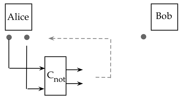
Since this is a 3-qubit system, Alice is really applying
$$\eqb{
& & \hspace{-20pt}
(\cnot \otimes I) \kt{T} \\
& \eql &
(\cnot \otimes I)
\isqts{1} \parenl{ \alpha\kt{000} + \alpha\kt{011}
+ \beta\kt{100} + \beta\kt{111} } \\
& \eql &
\isqts{1}
\parenl{ \alpha\cnot\kt{00}\kt{0} + \alpha\cnot\kt{01}\kt{1}
+ \beta\cnot\kt{10}\kt{0} + \beta\cnot\kt{11}\kt{1} } \\
& \eql &
\isqts{1}
\parenl{ \alpha\kt{000} + \alpha\kt{011}
+ \beta\kt{110} + \beta\kt{101} } \\
& \;\defn\; & \kt{T^\prime}
}$$
Here, we've named the result \(\kt{T^\prime}\).
- Step 4: Alice now applies \(H\otimes I \otimes I\):
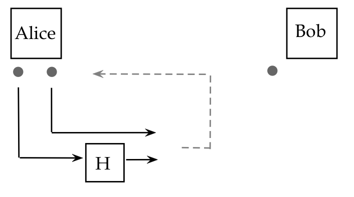
Thus, the net effect is:
$$\eqb{
\kt{T^{\prime\prime}}
& \eql &
(H\otimes I \otimes I) \kt{T^\prime} \\
& \eql &
(H\otimes I \otimes I)
\isqts{1}
\parenl{ \alpha\kt{000} + \alpha\kt{011}
+ \beta\kt{110} + \beta\kt{101} } \\
& \eql &
(H\otimes I \otimes I)
\isqts{1}
\parenl{ \alpha\kt{000} + \alpha\kt{011}
+ \beta\kt{110} + \beta\kt{101} } \\
& \eql &
\smf{1}{2}
\left(
\alpha \kt{000} + \alpha\kt{100} + \alpha\kt{011} + \alpha\kt{111}
\right. \\
& &
\left.
\beta\kt{010} - \beta\kt{110} + \beta\kt{001} - \beta\kt{101}
\right) \\
& \eql &
\smf{1}{2}
\left(
\alpha\kt{000} + \beta\kt{001} + \alpha\kt{011} + \beta\kt{010}
\right. \\
& &
\left.
\alpha\kt{100} - \beta\kt{101} + \alpha\kt{111} - \beta\kt{110}
\right) \\
}$$
Which simplifies to:
$$\eqb{
\kt{T^{\prime\prime}}
& \eql & & \smf{1}{2}
\kt{00} (\alpha\kt{0} + \beta\kt{1}) \\
& & + & \smf{1}{2}
\kt{01} (\alpha\kt{1} + \beta\kt{0}) \\
& & + & \smf{1}{2}
\kt{10} (\alpha\kt{0} - \beta\kt{1}) \\
& & + & \smf{1}{2}
\kt{11} (\alpha\kt{1} - \beta\kt{0}) \\
}$$
- Step 5: Alice measures both her qubits in the
standard basis:
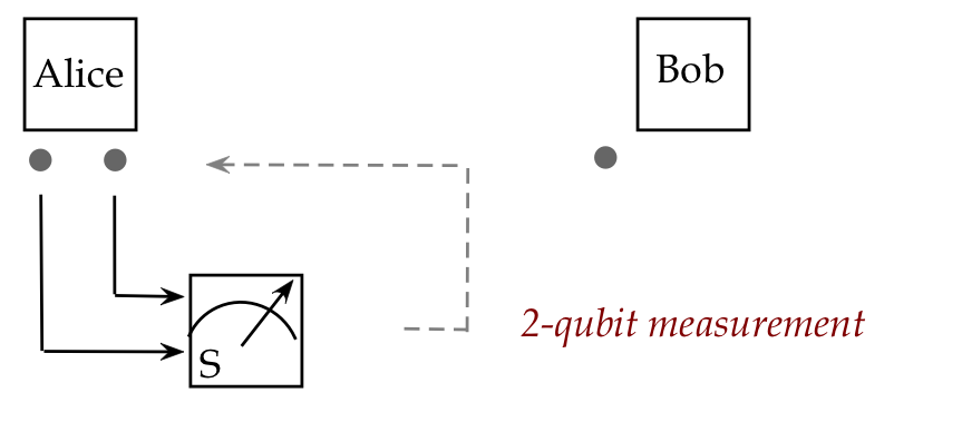
- Alice's 2-qubit measurement occurs with the projectors
$$\eqb{
P_{00} & \eql & \otr{00}{00} \\
P_{01} & \eql & \otr{01}{01} \\
P_{10} & \eql & \otr{10}{10} \\
P_{11} & \eql & \otr{11}{11} \\
}$$
- In the 3-qubit system with \(\kt{T^{\prime\prime}}\) as
the state, the projectors are then
$$\eqb{
P_{00} \otimes I & \eql & \otr{00}{00} \otimes I \\
P_{01} \otimes I & \eql & \otr{01}{01} \otimes I \\
P_{10} \otimes I & \eql & \otr{10}{10} \otimes I \\
P_{11} \otimes I & \eql & \otr{11}{11} \otimes I \\
}$$
- Alice then observes one of four S-basis states:
\(\kt{00}, \kt{01}, \kt{10}\) or \(\kt{11}\).
- However, the four possible 3-qubit outcomes
of Alice's measurement are:
$$\eqb{
\kt{00} & \otimes & (\alpha\kt{0} + \beta\kt{1}) \\
\kt{01} & \otimes & (\alpha\kt{1} + \beta\kt{0}) \\
\kt{10} & \otimes & (\alpha\kt{0} - \beta\kt{1}) \\
\kt{11} & \otimes & (\alpha\kt{1} - \beta\kt{0}) \\
}$$
- That is, Bob will end up with one of the
four qubit states on the right.
- Step 6: Alice communicates a classical value
to tell Bob which basis state resulted from measurement:
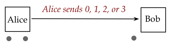
- If the outcome is \(\kt{00}\), she sends "0"
- If \(\kt{01}\), she sends "1"
- If \(\kt{10}\), she sends "2"
- If \(\kt{11}\), she sends "3"
This single message counts as two classical binary digits (bits).
- When Bob receives this information, he'll know
which of four unknown states
his qubit is in, but this is not the goal.
\(\rhd\)
Recall: neither of them know \(\alpha, \beta\).
- Bob will now transform his qubit without measuring
with the goal of transforming it to \(\alpha\kt{0} + \beta\kt{1}\).
- The following 1-qubit transforms achieve the goal:
$$\eqb{
I (\alpha\kt{0} + \beta\kt{1}) & \eql & (\alpha\kt{0} + \beta\kt{1})
& \mbx{if Alice sent "0"} \\
X (\alpha\kt{1} + \beta\kt{0}) & \eql & (\alpha\kt{0} + \beta\kt{1})
& \mbx{if Alice sent "1"} \\
Z (\alpha\kt{0} - \beta\kt{1}) & \eql & (\alpha\kt{0} + \beta\kt{1})
& \mbx{if Alice sent "2"} \\
iY (\alpha\kt{1} - \beta\kt{0}) & \eql & (\alpha\kt{0} + \beta\kt{1})
& \mbx{if Alice sent "3"} \\
}$$
- Step 7: Bob applies one of four transforms depending
on which classical message he receives:
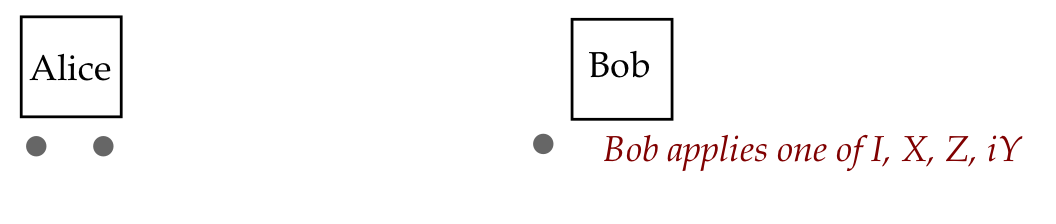
Note: Since this is a 3-qubit system,
Bob is really applying one of
$$\eqb{
(I \otimes I) \otimes I & \mbx{ for "0"} \\
(I \otimes I) \otimes X & \mbx{ for "1"} \\
(I \otimes I) \otimes Z & \mbx{ for "2"} \\
(I \otimes I) \otimes iY & \mbx{ for "3"} \\
}$$
- At this point:
- Bob's qubit is in the state \(\alpha\kt{0} + \beta\kt{1}\),
the original state of Alice's qubit.
- Alice's qubit state is destroyed (measured).
- Notice the key steps:
- Alice performs transforms where the numbers \(\alpha,\beta\)
apply to the entire three-qubit state.
- When she measures, the outcome is a standard vector,
leaving \(\alpha,\beta\) applying to Bob's qubit.
- Bob applies a non-destroying (unitary) transform to
adjust the qubit to Alice's original state.
- He needs to know which transform to apply: this comes
from the classical message.
- Thus, one could say that the state got transported
with the help of a classical message.
What does it all mean?
- Is this a fair use of the "beam me up" term teleportation?
- Some skepticism:
- It's not clear that the approach could work for anything
that constitutes matter.
- Even if matter could be unitarily transformed, how would
the entangled precursor be created?
- Even if a single molecule could be recreated, how can
one recreate the ensemble state of a collection of atoms?
- On the other hand ...
- It is true that only information was transferred.
- A full, unknown quantum state does in fact get recreated.
- Recent experiments
(example)
show that atoms can be created as entangled pairs.
- What do you think?
5.12*
Hermitian theory
Let's recall what we know about Hermitians and measurement so far:
- A Hermitian matrix "packages" projectors along with eigenvalues.
- For example, suppose a multi-qubit measurement consists
of projectors \(P_1, P_2, \ldots, P_k\).
- Then, for any choice of real numbers \(\lambda_1,\ldots,\lambda_k\),
the operator
$$
A \eql \sum_i \lambda_i P_i
$$
is Hermitian.
- In the simplest case, every projector is just an
outer-product
$$
P_i \eql \otr{\phi_i}{\phi_i}
$$
where \(\phi_i\) is a basis-vector of the measuring device.
- In this case, we could write
$$
A \eql \sum_i \lambda_i P_i
\eql \lambda_i \otr{\phi_i}{\phi_i}
$$
Here, the \(\phi_i\)'s now become the eigenvectors of \(A\),
with associated eigenvalues \(\lambda_i\) by this construction.
- Then, the single operator \(A\) contains all the information
for the measurement: the projectors and the eigenvalues that
correspond to real physical observed values.
Constructing multi-qubit Hermitians from smaller Hermitians:
- Recall: one can construct some larger projectors one qubit
at a time:
$$\eqb{
\otr{01}{01}
& \eql &
P_{01}
& \mbx{Projector for \(\kt{01}\) outcome} \\
& \eql &
P_0 \otimes P_1
& \mbx{Tensor product of smaller projectors} \\
& \eql &
\parenl{ I \otimes P_1 } \parenl{ P_0 \otimes I }
& \mbx{Apply \(P_0\) first, then \(P_1\)} \\
& \eql &
\parenl{ I \otimes \otr{1}{1} } \parenl{ \otr{0}{0} \otimes I }
& \mbx{The smaller ones as outerproducts}
}$$
- In the same way, because Hermitians tensor into larger
Hermitians, one can construct a larger Hermitian out of smaller ones:
$$\eqb{
A
& \eql & B \otimes C
& \mbx{2-qubit Hermitian \(A\) from tensoring 1-qubit Hermitians}\\
& \eql & \parenl{ I \otimes C } \parenl{B \otimes I}
& \mbx{Decomposition into stages} \\
}$$
Do the larger Hermitians package the tensored projectors from the
smaller ones?
- Indeed, they do. For example suppose
are two Hermitians that package the projectors for the $$\eqb{
A & \eql & \lambda_0\otr{0}{0} + \lambda_1\otr{1}{1} \\
B & \eql & \gamma_0\otr{0}{0} + \gamma_1\otr{1}{1} \\
}$$
first and second qubits.
- Then,
$$\eqb{
A \otimes B & \eql &
\parenl{ \lambda_0\otr{0}{0} + \lambda_1\otr{1}{1} }
\otimes
\parenl{ \gamma_0\otr{0}{0} + \gamma_1\otr{1}{1} } \\
& \eql &
\lambda_0\gamma_0 \parenl{ \otr{0}{0} \otimes \otr{0}{0} } \\
& &
+ \; \lambda_0\gamma_1 \parenl{ \otr{0}{0} \otimes \otr{1}{1} } \\
& &
+ \; \lambda_1\gamma_0 \parenl{ \otr{1}{1} \otimes \otr{0}{0} } \\
& &
+ \; \lambda_1\gamma_1 \parenl{ \otr{1}{1} \otimes \otr{1}{1} } \\
& \eql &
\lambda_0\gamma_0 \otr{00}{00}
+
\lambda_0\gamma_1 \otr{01}{01}
+
\lambda_1\gamma_0 \otr{10}{10}
+
\lambda_1\gamma_1 \otr{11}{11}
}$$
where we have used Proposition 4.4.
- These are exactly the eigenvectors and eigenvalues
of \(C = A\otimes B\) (Proposition 4.11)
How does any of this matter?
- For quantum computing algorithms,
Hermitians do not really matter because projectors are sufficient.
- Thus, the eigenvalues in the "packaging" do not matter
as long as different projectors have different eigenvalues.
- However, quantum computing hardware uses physical
devices governed by quantum mechanics.
- In this case, the actual physical observed values are
the eigenvalues.
\(\rhd\)
These come from the underlying physics of the system.
- When tensoring smaller systems, the resulting larger
system's eigenvalues can be expressed as products of the
smaller system's eigenvalues.
- Hermitians corresponding to different measurement types
can also be deployed in sequence:
- In this case, they may or may not share eigenvectors.
- If the eigenvectors are the same, the
measurements commute.
- In this case, the second measurement's outcome will be
the same as the first's outcome:
\(\rhd\)
There is certainty in the second outcome.
- Otherwise, the first measurement will result in probabilistic
outcomes for the second:
\(\rhd\)
Heisenberg's uncertainty principle.
- Hermitian theory is useful in analysis:
- For example, one can use the Hermitian sandwich to
calculate averages, what one should see in repeated
measurements of a physical system.
5.13*
Projectors, measurement and tensors - a rearview look
Let's return to measurement and crystallize projective measurement
into a few key concepts:
- First and most important: measurement = subspace projection
- Any measurement features three things:
- A collection of subspaces
- The act of measurement projects the input vector
on to one of the subspaces.
- The resulting normalized projected vector is the outcome (the new state).
Which particular subspace is determined randomly by nature
for each act of measurement,
based on the squared lengths of the projected vectors (the probabilities).
- For example, suppose we measure the first qubit
among three using the 1-qubit basis \(\kt{v},\kt{v^\perp}\).
- How many subspaces are now involved? Two, depending
on the outcome state of the first qubit.
- The other two qubits could potentially be in any states.
- Thus, there are two subspaces at work here:
$$\eqb{
V_1 & \eql & \mbox{span}
\setl{
\kt{v} \otimes \kt{0} \otimes \kt{0},
\kt{v} \otimes \kt{0} \otimes \kt{1},
\kt{v} \otimes \kt{1} \otimes \kt{0},
\kt{v} \otimes \kt{1} \otimes \kt{1}
} \\
V_2 & \eql & \mbox{span}
\setl{
\kt{v^\perp} \otimes \kt{0} \otimes \kt{0},
\kt{v^\perp} \otimes \kt{0} \otimes \kt{1},
\kt{v^\perp} \otimes \kt{1} \otimes \kt{0},
\kt{v^\perp} \otimes \kt{1} \otimes \kt{1}
}
}$$
- Which we could shorten to:
$$\eqb{
V_1 & \eql & \mbox{span}
\setl{
\kt{v,0,0},
\kt{v,0,1},
\kt{v,1,0},
\kt{v,1,1}
} \\
V_2 & \eql & \mbox{span}
\setl{
\kt{v^\perp, 0, 0},
\kt{v^\perp, 0, 1},
\kt{v^\perp, 1, 0},
\kt{v^\perp, 1, 1}
}
}$$
- What are the projectors in the example above?
- Since there are two subspaces, there will be two
projectors.
- A projector for a subspace is the sum of projectors
of its basis vectors.
- Thus, the two subspace projectors are:
$$\eqb{
P_{V_1} & \eql &
\otr{v,0,0}{v,0,0}
\: + \: \otr{v,0,1}{v,0,1}
\: + \: \otr{v,1,0}{v,1,0}
\: + \: \otr{v,1,1}{v,1,1} \\
P_{V_2} & \eql &
\otr{v^\perp,0,0}{v^\perp,0,0}
\: + \: \otr{v^\perp,0,1}{v^\perp,0,1}
\: + \: \otr{v^\perp,1,0}{v^\perp,1,0}
\: + \: \otr{v^\perp,1,1}{v^\perp,1,1}
}$$
- The rest is calculation:
- For input vector \(\ksi\)
$$\eqb{
\mbox{Outcome } &
\smf{1}{\mag{P_{V_1}\ksi}} P_{V_1}\ksi
& \mbox{ occurs with probability } &
\magsq{P_{V_1}\ksi} \\
\mbox{Outcome } &
\smf{1}{\mag{P_{V_2}\ksi}} P_{V_2}\ksi
& \mbox{ occurs with probability } &
\magsq{P_{V_2}\ksi} \\
}$$
- Alternatively, for notational practice, let's also write this as:
$$\eqb{
\mbox{Outcome } &
\smf{1}{\sqrt{\swich{\psi}{P_{V_1}}{\psi}}} P_{V_1}\ksi
& \mbox{ occurs with probability } &
\swich{\psi}{P_{V_1}}{\psi} \\
\mbox{Outcome } &
\smf{1}{\sqrt{\swich{\psi}{P_{V_2}}{\psi}}} P_{V_2}\ksi
& \mbox{ occurs with probability } &
\swich{\psi}{P_{V_2}}{\psi} \\
}$$
- Consider another example: suppose we
performed a Bell-basis measurement on the first two of three qubits:
- Recall the Bell basis:
$$\eqb{
\kt{\Phi^+} & \eql & \isqts{1} \parenl{ \kt{00} + \kt{11} } \\
\kt{\Phi^-} & \eql & \isqts{1} \parenl{ \kt{00} - \kt{11} } \\
\kt{\Psi^+} & \eql & \isqts{1} \parenl{ \kt{01} + \kt{10} } \\
\kt{\Psi^-} & \eql & \isqts{1} \parenl{ \kt{01} - \kt{10} } \\
}$$
- How many subspaces? There are four outcomes for the first two
qubits.
- The third qubit could be in any state.
- Thus, the four projection subspaces are:
$$\eqb{
W_1 & \eql & \mbox{span}
\setl{\kt{\Phi^+, 0}, \kt{\Phi^+, 1} } \\
W_2 & \eql & \mbox{span}
\setl{\kt{\Phi^-, 0}, \kt{\Phi^-, 1} } \\
W_3 & \eql & \mbox{span}
\setl{\kt{\Psi^+, 0}, \kt{\Psi^+, 1} } \\
W_4 & \eql & \mbox{span}
\setl{\kt{\Psi^-, 0}, \kt{\Psi^-, 1} } \\
}$$
- And, therefore, the four projectors are:
$$\eqb{
P_{W_1} & \eql &
\otr{\Phi^+, 0}{\Phi^+, 0} \: + \: \otr{\Phi^+, 1}{\Phi^+, 1} \\
P_{W_2} & \eql &
\otr{\Phi^-, 0}{\Phi^-, 0} \: + \: \otr{\Phi^-, 1}{\Phi^-, 1} \\
P_{W_3} & \eql &
\otr{\Psi^+, 0}{\Psi^+, 0} \: + \: \otr{\Psi^+, 1}{\Psi^+, 1} \\
P_{W_4} & \eql &
\otr{\Psi^-, 0}{\Psi^-, 0} \: + \: \otr{\Psi^-, 1}{\Psi^-, 1} \\
}$$
- Finally, let's examine how tensoring can build
projectors:
- In the first example:
$$\eqb{
P_{V_1} & \eql &
\otr{v}{v} \otimes I \otimes I \\
P_{V_2} & \eql &
\otr{v^\perp}{v^\perp} \otimes I \otimes I \\
}$$
(To prove this, expand \(I\) in Dirac form and work through the algebra.)
- In the second example:
$$\eqb{
P_{W_1} & \eql &
\otr{\Phi^+}{\Phi^+} \otimes I \\
P_{W_2} & \eql &
\otr{\Phi^-}{\Phi^-} \otimes I \\
P_{W_3} & \eql &
\otr{\Psi^+}{\Psi^+} \otimes I \\
P_{W_4} & \eql &
\otr{\Psi^-}{\Psi^-} \otimes I \\
}$$
Here, each is a tensor of a 2-qubit outer-product with
a 1-qubit identity.
- That, in a nutshell, is nearly all of what we need to know
about measurement.
- There is a small variation we will see later called
Pauli measurement that will be useful for one application.
Lastly, a note about tensored Dirac notation:
- Earlier, we wrote the short form
$$
\kt{v} \otimes \kt{0} \otimes \kt{0},
\eql \kt{v,0,0}
$$
- An alternative way to write the same:
$$
\kt{v} \otimes \kt{0} \otimes \kt{0},
\eql \kt{v} \kt{0} \kt{0}
$$
- However, this can make outerproducts confusing, for example:
$$
\kt{v} \kt{0} \kt{0} \br{v}\br{0}\br{0}
$$
This is really intended to be
$$
\parenl{ \kt{v} \kt{0} \kt{0} } \parenl{ \br{v}\br{0}\br{0} }
$$
- It's better to use the comma-separation for outerproducts:
$$
\otr{v,0,0}{v,0,0}
$$
- The \(\kt{v} \kt{0} \kt{0}\) form is more commonly used
when applying operators as in:
$$
(I \otimes I \otimes X) \kt{v} \kt{0} \kt{0}
\eql
\kt{v} \kt{0} \kt{1}
$$
Don't forget: Module-5 solved problems