Module objectives
In this module, our aim is to extend the theory towards multiple
qubits and their interactions:
- Tensor products for vectors
- Tensor products for operators
- Extension of properties: projector, Hermitian, unitary.
- Entanglement
4.1
What do we call a group of interacting qubits?
Let's first examine the same question for classical bits:
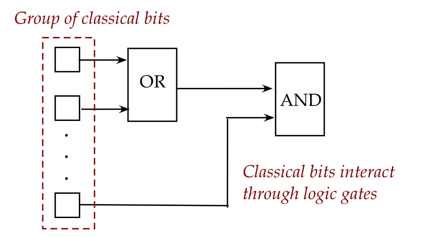
- In classical logic, multiple bits interact through logic gates.
- For example:
- Let's think of the (classical) bit as a device that can
hold one of the values (states) \(0\) or \(1\).
- At any given moment, a bit can either be in state \(0\) or in
state \(1\).
- Interactions are arranged through logic gates.
- What happens to the outputs?
- Some of the outputs can come back and be used to replace
the state of a bit.
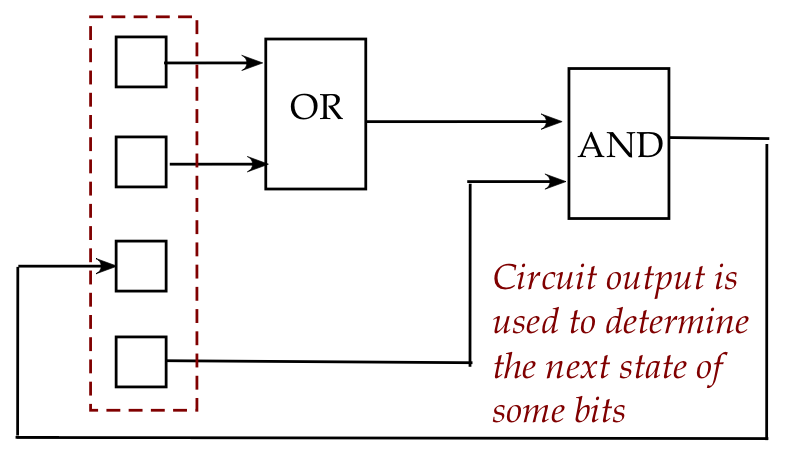
- But alternatively, some outputs can be made to change other
bits (not pictured).
- We typically use the term register for
a group of classical bits that are primed for interaction.
- Note: there's no sense in which a group of bits can be
considered a "larger bit".
Let's now ask the same question about qubits:
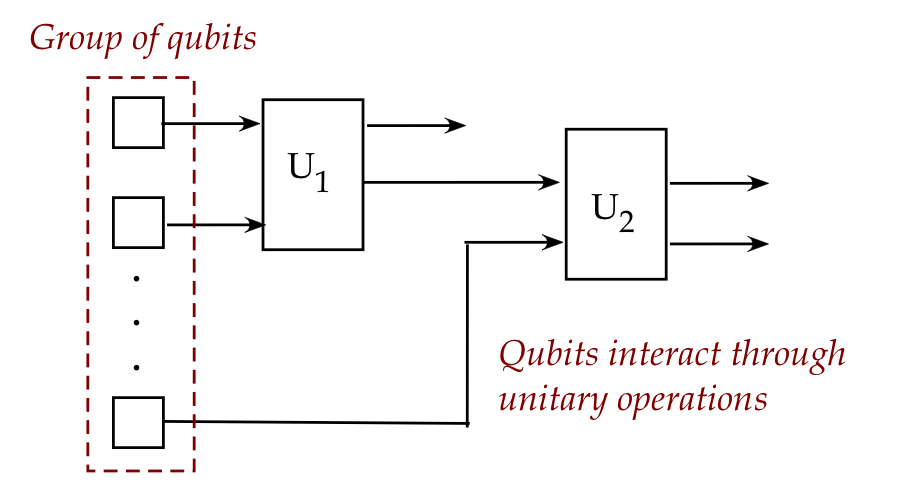
- Here, the devices are qubits and the values (states) they can hold
are complex 2D vectors.
- At any given moment, a qubit's state can be any valid
unit-length 2D vector such as \(\ksi = \alpha\kt{0} + \beta\kt{1}\).
- Interactions between qubits are arranged through unitary
operations that change the qubits directly
(as opposed to changing other qubits.)
- Now for the surprise:
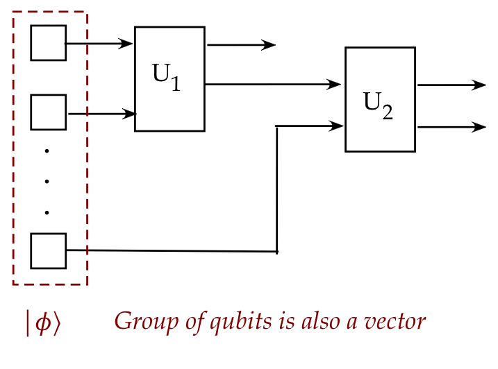
- A group of qubits, each a 2-component vector,
is itself a larger vector.
- The whole group of qubits can be treated as a single vector
with a single combined state.
- This was not possible with classical bits.
Does it matter?
- It certainly does, in many ways.
- First, as we will see in this module, the entire theory
of linear algebra we developed for single qubits extends to
the vectors and unitary operations for multiple qubits.
- But there are surprising implications to this larger vector
for the group of qubits.
- Suppose we use the standard basis to represent the
individual vectors in a three qubit example:
- One possible set of values is: \(\kt{0}, \kt{0}, \kt{0}\).
\(\rhd\)
We write the combined vector as \(\kt{000}\).
- Another possible set is: \(\kt{1}, \kt{0}, \kt{1}\).
\(\rhd\)
The combined vector is \(\kt{101}\).
- In this way, it will turn out that the larger vector space
has an 8-vector basis:
\(\kt{000}, \kt{001}, \kt{010},\ldots, \kt{110},\kt{111}\).
- Now for the first surprising implication:
- With the three-qubit example, because there are 8 basis
vectors, any unit-length linear combination is also a valid state,
e.g.
$$
\frac{1}{\sqrt{8}} (\kt{000} + \kt{001} + \ldots + \kt{111})
$$
- Thus, with \(n\) qubits, any (unit-length) linear combination
of \(2^n\) basis vectors is a potential state.
- Compare with classical:
- Classical: \(n\) bits can hold one of \(2^n\) combinations,
\(\rhd\)
Each state is an n-bit binary combination.
- Quantum: \(n\) qubits can hold one of an uncountable
number linear combinations,
\(\rhd\)
Each state is a linear combination of \(2^n\) basis vectors.
Thus, a single quantum state for n-qubits has the potential
to be exponentially larger than a single classical state!
- We will later see that an equal-weight combination of
all \(2^n\) basis vectors is in fact a starting state common
to many algorithms.
Entanglement: the other surprise
- Consider a two-qubit system in the state
$$
\ksi \eql \isqt{1} (\kt{01} + \kt{10})
$$
(What precisely this means we will see later.)
- Thus, what we can infer is, when measured in the standard
basis:
- First qubit state = \(\kt{0}\) \(\iff\) \(\kt{1}\) = second
qubit state.
- First qubit state = \(\kt{1}\) \(\iff\) \(\kt{0}\) = second
qubit state.
- It can never be that they are both in the same state.
- What is profoundly interesting (and useful) is that
the two qubits above can be physically separated while
maintaining this property.
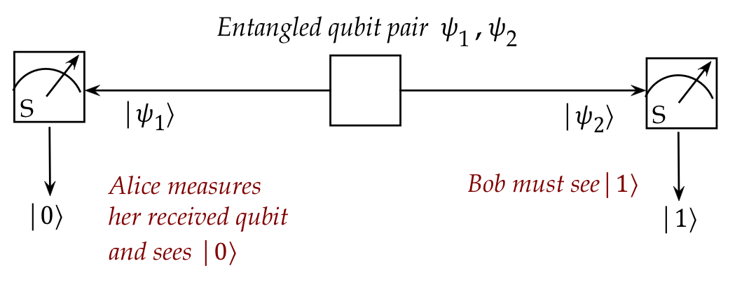
- Then, if Alice measures the first qubit, the outcome exactly
determines what Bob sees with the second qubit.
\(\rhd\)
Instantaneously, no matter the distance between Alice and Bob.
- Indeed, this feature (which Einstein called "spooky")
is exploited in communication protocols.
Thus, the goal of this module is to develop the theory that
connects the larger multi-qubit vector from the individual qubit vectors.
For this, we need a new linear algebra construct:
the tensor product.
4.2
Tensor products of vectors
A tensor product of two vectors (for the two qubit case)
creates a larger vector.
Let's use a simple two-qubit example to see what's needed to build this
larger vector:
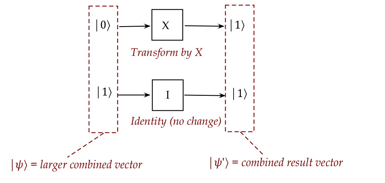
- In this setup:
- The first qubit is flipped via the \(X\) operator.
- The second qubit remains the same
\(\rhd\)
This is the same as applying the identity operator \(I\).
- Looked at individually, we would write
$$\eqb{
X \kt{0}
& \eql &
\mat{0 & 1\\1 & 0} \vectwo{1}{0}
& \eql &
\vectwo{0}{1} \\
I \kt{1}
& \eql &
\mat{1 & 0\\0 & 1} \vectwo{0}{1}
& \eql &
\vectwo{0}{1} \\
}$$
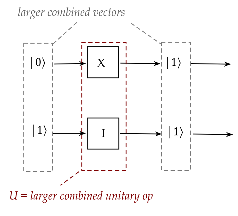
- Suppose we had
- A larger vector \(\ksi\) that described the initial
combined state of the qubits.
- A larger vector \(\kt{\psi^\prime}\) for the result
- A larger unitary operator \(U\) to achieve the combined
transformation
Then, we must have
$$
U \ksi \eql \kt{\psi^\prime}
$$
- As it turns out, this is exactly what will transpire:
$$
U \ksi
\eql
\mat{0 & 0 & 1 & 0\\
0 & 0 & 0 & 1\\
1 & 0 & 0 & 0\\
0 & 1 & 0 & 0}
\mat{0\\ 1\\ 0\\ 0}
\eql
\mat{0\\ 0\\ 0\\ 1}
\eql
\kt{\psi^\prime}
$$
- Recall: the input of the circuit was \(\kt{0}\) and \(\kt{1}\).
- The vector \(\ksi\) is not \(\kt{0}\) and \(\kt{1}\)
stacked one on top of the other. That is,
$$
\ksi \eql \mat{0\\ 1\\ 0\\ 0} \; \neq \;
\left[
\begin{array}{c} 1\\ 0\\\hline 0\\ 1 \end{array}
\right]
$$
- Similarly, with the output of the circuit being
\(\kt{1}\) and \(\kt{1}\),
$$
\kt{\psi^\prime} \; \neq \;
\left[
\begin{array}{c} 0\\ 1\\\hline 0\\ 1 \end{array}
\right]
$$
The larger vector, in fact, is constructed in a different way:
through the tensor product.
- We will devise special notation to combine vectors and
operators:
\(\rhd\)
The tensor symbol \(\otimes\)
- Think of the tensor symbol \(\otimes\) as "combining across qubits"
- We will combine two single-qubit vectors into a larger 2-qubit
vector, as in
$$\eqb{
\ksi & \eql & \kt{0} \otimes \kt{1} \eql \mat{0\\ 1\\ 0\\ 0}\\
\kt{\psi^\prime} & \eql & \kt{1} \otimes \kt{1} \eql \mat{0\\ 0\\ 0\\ 1}\\
}$$
- And we will combine two single-qubit operators into a larger
2-qubit operator, as in:
$$\eqb{
U & \eql & X \otimes I \eql
\mat{0 & 0 & 1 & 0\\
0 & 0 & 0 & 1\\
1 & 0 & 0 & 0\\
0 & 1 & 0 & 0}
}$$
- Just how this tensoring works ... that's the next step.
Next, let's ask: what kinds of properties are desirable or
necessary for tensors?
- The first property, one that we will impose, is distribution
of \(\otimes\) over addition:
- Given individual vectors \(\kt{v_1}, \kt{v_2}, \kt{w}\) the
following needs to be true:
$$
\parenh{\kt{v_1} + \kt{v_2}} \otimes \kt{w}
\eql
\parenh{\kt{v_1} \otimes \kt{w}}
\: + \: \parenh{\kt{v_2} \otimes \kt{w}}
$$
- And symmetrically
$$
\kt{w} \otimes \parenh{\kt{v_1} + \kt{v_2}}
\eql
\parenh{\kt{w} \otimes \kt{v_1}}
\: + \: \parenh{\kt{w} \otimes \kt{v_2}}
$$
- Such a property is verifiable experimentally.
- Once we accept distribution, we see that
$$
2\kt{v} \otimes \kt{w}
\eql
\parenh{\kt{v} + \kt{v}} \otimes \kt{w}
\eql
\parenh{\kt{v} \otimes \kt{w}}
\: + \: \parenh{\kt{v} \otimes \kt{w}}
\eql
2 \parenh{\kt{v} \otimes \kt{w}}
$$
In general, this would also mean
$$
(k \kt{v}) \otimes \kt{w}
\eql
k (\kt{v} \otimes \kt{w})
\eql (\kt{v} \otimes k \kt{w}
$$
for any integer \(k\).
- It would have to be a very strange operation to
only work for integers, so in general:
$$
(\alpha \kt{v}) \otimes \kt{w}
\eql
\alpha (\kt{v} \otimes \kt{w})
\eql (\kt{v} \otimes \alpha \kt{w}
$$
for any complex number \(\alpha\).
- With these requirements on \(\otimes\) we are almost safely
in the comfort zone of traditional linearity:
$$\eqb{
\parenh{ \alpha\kt{v_1} + \beta\kt{v_2} } \otimes \kt{w}
& \eql &
\alpha \parenh{ \kt{v_1} \otimes \kt{w} }
+
\beta \parenh{ \kt{v_2} \otimes \kt{w} } \\
\parenh{ \kt{w} \otimes \alpha\kt{v_1} + \beta\kt{v_2} }
& \eql &
\alpha \parenh{ \kt{w} \otimes \kt{v_1} }
+
\beta \parenh{ \kt{w} \otimes \kt{v_2} }
}$$
- Why did we say almost?
- Recall from above:
$$
\alpha (\kt{v} \otimes \kt{w})
\eql
(\alpha \kt{v}) \otimes \kt{w}
\eql (\kt{v} \otimes \alpha \kt{w})
\neq
(\alpha \kt{v} \otimes \alpha \kt{w})
$$
- That is, the scalar \(\alpha\) when pushed inside the tensor
product attaches to only one of the operands.
- Either the left operand or the right, but not both.
- In fact
$$
(\alpha \kt{v} \otimes \alpha \kt{w})
\eql
\alpha^2 (\kt{v} \otimes \kt{w})
$$
- We can then push two scalars differently, as in:
$$
\alpha\beta \parenh{ \kt{v} \otimes \kt{w} }
\eql
\alpha \kt{v} \otimes \beta \kt{w}
$$
or
$$
\alpha\beta \parenh{ \kt{v} \otimes \kt{w} }
\eql
\beta \kt{v} \otimes \alpha \kt{w}
$$
- This property is called bilinearity.
- With operators, however, the order in bilinearity matters, as in:
$$
\parenh{X \otimes I} \parenh{\kt{0} \otimes \kt{1}}
\eql
\parenh{X \kt{0} \otimes I \kt{1}}
\eql
\parenh{\kt{1} \otimes \kt{1}}
$$
More about this in the next section.
Next, with 2-qubit examples,
let's now figure out how to build the larger vectors:
- We know that a single-qubit vector has two coordinates because
it's a 2D vector, as in:
$$
\kt{1} \eql \vectwo{0}{1}
$$
- Thus, when we combine two such vectors (one per qubit),
we'll have four numbers
\(\rhd\)
That is, a 4-component vector.
- The standard basis for 4-component vectors is:
$$
\mat{1\\ 0\\ 0\\ 0}
\;\;\;\;\;\;\;\;
\mat{0\\ 1\\ 0\\ 0}
\;\;\;\;\;\;\;\;
\mat{0\\ 0\\ 1\\ 0}
\;\;\;\;\;\;\;\;
\mat{0\\ 0\\ 0\\ 1}
$$
- Now, the basis vectors for each individual qubit are
$$
\vectwo{1}{0}
\;\;\;\;\;\;\;\;
\vectwo{0}{1}
$$
- So, somehow the four possible combinations of these
need to produce the four larger basis vectors:
$$
\vectwo{1}{0}
\otimes
\vectwo{1}{0}
\eql
\mat{1\\ 0\\ 0\\ 0}
\;\;\;\;\;\;\;\;
\vectwo{1}{0}
\otimes
\vectwo{0}{1}
\eql
\mat{0\\ 1\\ 0\\ 0}
\;\;\;\;\;\;\;\;
\vectwo{0}{1}
\otimes
\vectwo{1}{0}
\eql
\mat{0\\ 0\\ 1\\ 0}
\;\;\;\;\;\;\;\;
\vectwo{0}{1}
\otimes
\vectwo{0}{1}
\eql
\mat{0\\ 0\\ 0\\ 1}
$$
That is we need to figure out: what rule takes two smaller vectors
to produce the larger?
- The answer comes from bilinearity:
- Let's look at
$$
\vectwo{\alpha_1}{0}
\otimes
\vectwo{\beta_1}{0}
\eql
\alpha_1 \vectwo{1}{0}
\otimes
\beta_1 \vectwo{1}{0}
\eql
\alpha_1 \beta_1 \mat{1\\ 0\\ 0\\ 0}
\eql
\mat{\alpha_1 \beta_1 \\ 0\\ 0\\ 0}
$$
- And
$$
\vectwo{\alpha_1}{0}
\otimes
\vectwo{0}{\beta_2}
\eql
\alpha_1 \vectwo{1}{0}
\otimes
\beta_2 \vectwo{0}{1}
\eql
\alpha_1 \beta_2 \mat{0\\ 1\\ 0\\ 0}
\eql
\mat{0\\ \alpha_1 \beta_2 \\ 0\\ 0}
$$
where we're naming the constants in a certain way to clarify what
comes next.
- Let's do the remaining two:
$$
\vectwo{0}{\alpha_2}
\otimes
\vectwo{\beta_1}{0}
\eql
\alpha_2 \vectwo{0}{1}
\otimes
\beta_1 \vectwo{1}{0}
\eql
\alpha_2 \beta_1 \mat{0\\ 0\\ 1\\ 0}
\eql
\mat{0\\ 0\\ \alpha_2 \beta_1 \\ 0}
$$
and
$$
\vectwo{0}{\alpha_2}
\otimes
\vectwo{0}{\beta_2}
\eql
\alpha_2 \vectwo{0}{1}
\otimes
\beta_2 \vectwo{0}{1}
\eql
\alpha_2 \beta_2 \mat{0\\ 0\\ 0\\ 1}
\eql
\mat{0\\ 0\\ 0\\ \alpha_2 \beta_2}
$$
- Adding on both sides gives us
$$
\vectwo{\alpha_1}{\alpha_2}
\otimes
\vectwo{\beta_1}{\beta_2}
\eql
\mat{\alpha_1 \beta_1\\ \alpha_1 \beta_2\\ \alpha_2 \beta_1\\ \alpha_2 \beta_2}
$$
which, for insight, we can also write as:
$$
\vectwo{\alpha_1}{\alpha_2}
\otimes
\vectwo{\beta_1}{\beta_2}
\eql
\mat{\alpha_1 \mat{\beta_1\\ \beta_2} \\ \alpha_2\mat{\beta_1\\ \beta_2}}
$$
Thus, each element of the first vector multiplies into the
entire other vector, and all these are stacked up.
- We now have our rule for computing
\(\kt{v}\otimes\kt{w}\) for any two 2D vectors
\(\kt{v}\) and \(\kt{w}\).
- The same idea can be generalized to n dimensions:
$$
\vecthree{\alpha_1}{\vdots}{\alpha_n}
\otimes
\vecthree{\beta_1}{\vdots}{\beta_n}
\eql
\mat{ \alpha_1 \mat{\beta_1 \\ \vdots \\ \beta_n} \\
\alpha_2 \mat{\beta_1 \\ \vdots \\ \beta_n} \\
\vdots \\
\alpha_n \mat{\beta_1 \\ \vdots \\ \beta_n} }
\eql
\mat{\alpha_1 \beta_1\\ \vdots \\ \alpha_1 \beta_n \\
\alpha_2 \beta_1\\ \vdots \\ \alpha_2 \beta_n \\ \vdots \\
\alpha_n \beta_1\\ \vdots \\ \alpha_n \beta_n }
$$
- This is called the vector tensor product.
- Note: none of the number-products involve conjugation.
In-Class Exercise 1:
Compute the following tensor products in column format:
- \(\kt{+}\otimes\kt{+}\)
- \(\kt{+}\otimes\kt{0}\)
Inner product:
- Now that we've defined the tensor product to be a vector,
that larger vector will have an inner product
- For example:
- Suppose
$$
\ksi \eql \kt{v}\otimes\kt{w}
$$
is one tensored vector.
- And let
$$
\kt{\phi} \eql \kt{x}\otimes\kt{y}
$$
be another.
- Clearly, since \(\ksi\) and \(\kt{\phi}\) are same-size vectors,
we can compute the inner product
$$
\inr{\psi}{\phi}
$$
- Now, in the example above, one can compute inner products
of the small vectors \(\kt{v}, \kt{w}, \kt{x}, \kt{y}\) in
various combinations.
- Thus, the key question is: can we relate
\(\inr{\psi}{\phi}\) to the inner products of the smaller vectors?
- The answer is: yes
$$
\inr{\psi}{\phi}
\eql
\inrh{ \kt{v} \otimes \kt{w}}{ \kt{x} \otimes \kt{y} }
\eql
\parenh{ \inr{v}{x} } \parenh{ \inr{w}{y} }
$$
- To get some insight into why, let's examine
$$\eqb{
\inrh{ \alpha_1 \kt{0} \otimes \beta_1 \kt{0}}{ \gamma_1
\kt{0} \otimes \delta_1 \kt{0} }
& \eql &
\left( \vectwo{\alpha_1}{0} \otimes \vectwo{\beta_1}{0} \right)^\dagger
\left( \vectwo{\gamma_1}{0} \otimes \vectwo{\delta_1}{0} \right) \\
& \eql &
\left( \mat{\alpha_1 \beta_1 \\ 0 \\ 0 \\ 0} \right)^\dagger
\left( \mat{\gamma_1 \delta_1 \\ 0 \\ 0 \\ 0} \right) \\
& \eql &
\alpha_1^* \beta_1^* \gamma_1 \delta_1
}$$
-
Now we can write the latter as
$$
(\alpha_1^* \gamma_1) \: (\beta_1^* \delta_1)
$$
- This is the direct number-product of the two smaller
inner products:
$$
(\alpha_1^* \gamma_1) \: (\beta_1^* \delta_1)
\eql
\left(
\mat{\alpha_1 \\ 0}^\dagger
\mat{\gamma_1 \\ 0}
\right)
\left(
\mat{\beta_1 \\ 0}^\dagger
\mat{\delta_1 \\ 0}
\right)
\eql
(\inr{v}{x}) \: (\inr{w}{y})
$$
- In this way, one can work out the inner product for
any linear combination of the basis vectors the inner product.
- One minor point about convention:
- When we re-grouped
$$
\alpha_1^* \beta_1^* \gamma_1 \delta_1
\eql
(\alpha_1^* \gamma_1) \: (\beta_1^* \delta_1)
$$
we could have alternatively re-grouped as
$$
\alpha_1^* \beta_1^* \gamma_1 \delta_1
\eql
(\alpha_1^* \delta_1) \: (\beta_1^* \gamma_1)
$$
and defined a different type of inner product.
- But this would deviate from the left-to-right order
we have been using so far.
- Hence the convention is to define the larger
inner product as
$$
\inrh{ \kt{v} \otimes \kt{w}}{ \kt{x} \otimes \kt{y} }
\eql
\parenh{ \inr{v}{x} } \parenh{ \inr{w}{y} }
$$
- We will occasionally also write the larger inner product as
$$
\inrh{ \br{v} \otimes \br{w}}{ \kt{x} \otimes \kt{y} }
$$
where it should be understood that the left side
row-conjugation is performed just once.
- In fact, to avoid a thicket of brackets, one often writes the larger
inner product more simply as:
$$
\inrh{v \otimes w}{ x \otimes y } \eql
\inr{v}{x} \: \inr{w}{y}
$$
In-Class Exercise 2:
Evaluate the inner product
\( \inrh{ \kt{0} \otimes \kt{+}}{ \kt{+} \otimes \kt{0} } \).
4.3
Tensor products of operators
Let's turn to building larger, tensored matrices from smaller ones:
- Let's first describe what we seek:
- Suppose we have a tensor product like
$$
\kt{v} \otimes \kt{w}
$$
- And suppose we have unitary operators acting on each qubit,
as in
$$
A\kt{v} \otimes B\kt{w}
$$
- This will result in a larger vector.
- What we want is to figure out the larger matrix \(C\) such that
$$
C \: (\kt{v} \otimes \kt{w})
\eql
A\kt{v} \otimes B\kt{w}
$$
- What we really need is the relationship between \(C\) and
\(A\) and \(B\).
- The relationship is readily obtained through a bit
of painstaking multiplication.
- Let's start with the smaller products:
- Suppose
$$
\kt{v} = \vectwo{v_1}{v_2}
\;\;\;\;\;\;\;\;
\kt{w} = \vectwo{w_1}{w_2}
$$
and
$$
A \eql \mat{a_{11} & a_{12} \\
a_{21} & a_{22}}
\;\;\;\;\;\;\;\;
B \eql \mat{b_{11} & b_{12} \\
b_{21} & b_{22}}
$$
- Note: the indices \(1\) and \(2\) in \(v_1, v_2\) range over
the elements (coordinates) inside vectors.
- Then
$$\eqb{
A\kt{v} \otimes B\kt{w}
& \eql &
\mat{a_{11}v_1 + a_{12}v_2 \\
a_{21}v_1 + a_{22}v_2 }
\;\;\otimes \;\;
\mat{b_{11}w_1 + b_{12}w_2 \\
b_{21}w_1 + b_{22}w_2} \\
& & \\
& \eql &
\mat{
(a_{11}v_1 + a_{12}v_2) \mat{b_{11}w_1 + b_{12}w_2 \\
b_{21}w_1 + b_{22}w_2} \\
(a_{21}v_1 + a_{22}v_2) \mat{b_{11}w_1 + b_{12}w_2 \\
b_{21}w_1 + b_{22}w_2}
} \\
& & \\
& \eql & \ldots \mbox{ a few steps } \ldots \\
& & \\
& \eql &
\mat{
a_{11} \mat{b_{11} & b_{12} \\
b_{21} & b_{22}}
&
a_{12} \mat{b_{11} & b_{12} \\
b_{21} & b_{22}} \\
a_{21} \mat{b_{11} & b_{12} \\
b_{21} & b_{22}}
&
a_{22} \mat{b_{11} & b_{12} \\
b_{21} & b_{22}}
}
\mat{ v_1 w_1 \\ v_1 w_2 \\ v_2 w_1 \\ v_2 w_2 } \\
& & \\
& \eql &
\mat{
a_{11} \mat{b_{11} & b_{12} \\
b_{21} & b_{22}}
&
a_{12} \mat{b_{11} & b_{12} \\
b_{21} & b_{22}} \\
a_{21} \mat{b_{11} & b_{12} \\
b_{21} & b_{22}}
&
a_{22} \mat{b_{11} & b_{12} \\
b_{21} & b_{22}}
}
\;\; \kt{v} \otimes \kt{w}
}$$
- Thus,
$$
C
\eql
\mat{
a_{11} \mat{b_{11} & b_{12} \\
b_{21} & b_{22}}
&
a_{12} \mat{b_{11} & b_{12} \\
b_{21} & b_{22}} \\
a_{21} \mat{b_{11} & b_{12} \\
b_{21} & b_{22}}
&
a_{22} \mat{b_{11} & b_{12} \\
b_{21} & b_{22}}
}
$$
In terms of the elements of \(A\) and \(B\):
$$
\mat{a_{11} & a_{12} \\
a_{21} & a_{22}}
\;\otimes \;
\mat{b_{11} & b_{12} \\
b_{21} & b_{22}}
\; \eql \;
\mat{
a_{11} \mat{b_{11} & b_{12} \\
b_{21} & b_{22}}
&
a_{12} \mat{b_{11} & b_{12} \\
b_{21} & b_{22}} \\
a_{21} \mat{b_{11} & b_{12} \\
b_{21} & b_{22}}
&
a_{22} \mat{b_{11} & b_{12} \\
b_{21} & b_{22}}
}
$$
- We now have a way to tensor matrices.
- We will use the same notation as we did with vectors and
define
$$
C \eql A \otimes B
$$
- The derivation above also showed that
$$
(A \otimes B) \: (\kt{v} \otimes \kt{w})
\eql
(A \kt{v} \otimes B \kt{w})
$$
which is a form of bilinearity for operators.
- Here, the order of \(A\) and \(B\) matters: in general
$$
A \otimes B \; \neq \; B \otimes A
$$
- The same idea generalizes to n dimensions:
$$
A \otimes B
\eql
\mat{
a_{11}
\mat{b_{11} & \ldots & b_{1n} \\
\vdots & \vdots & \vdots \\
b_{n1} & \vdots & b_{nn}}
& \ldots &
a_{1n}
\mat{b_{11} & \ldots & b_{1n} \\
\vdots & \vdots & \vdots \\
b_{n1} & \vdots & b_{nn}} \\
\vdots & \vdots & \vdots \\
a_{n1}
\mat{b_{11} & \ldots & b_{1n} \\
\vdots & \vdots & \vdots \\
b_{n1} & \vdots & b_{nn}}
& \ldots &
a_{nn}
\mat{b_{11} & \ldots & b_{1n} \\
\vdots & \vdots & \vdots \\
b_{n1} & \vdots & b_{nn}} \\
}
$$
In-Class Exercise 3:
Fill in the missing steps in the matrix tensor derivation above.
In-Class Exercise 4:
Write down the single qubit matrices
\(\otr{0}{0}, \otr{1}{1}\), and then calculate
$$
\otr{0}{0} \otimes I \; + \; \otr{1}{1} \otimes X
$$
where \(X = \mat{0 & 1\\ 1 & 0}\). The result is
one of the most important operators in quantum computing
called \(\cnot\).
In-Class Exercise 5:
Recall that
\(H\) is the Hadamard operator
\(H = \mat{\isqt{1} & \isqt{1}\\
\isqt{1} & -\isqt{1}} \)
- Compute and compare \(H\kt{0} \otimes H\kt{0}\) and
\( \parenl{ H \otimes H } \parenl{ \kt{0} \otimes \kt{0} }\)
- Show that
\( \parenl{ H \otimes H } \parenl{ \kt{0} \otimes \kt{0} }
= \frac{1}{2} \parenl{ \kt{0} \otimes \kt{0} + \kt{0} \otimes \kt{1} +
\kt{1} \otimes \kt{0} + \kt{1} \otimes \kt{1} }\)
Summary so far:
- We have seen how two vectors representing two qubits
can be combined into a single vector for both:
- We've also seen how to combine unitary operators,
which we can think of as:
- What we'd like is to extend the theory so that:
- It naturally handles \(n\) qubits through the same tensor
product, as in:
$$
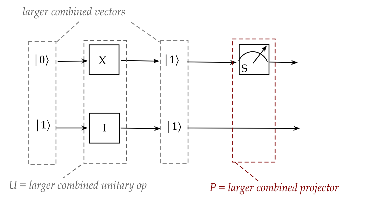
\kt{v} \eql \kt{v_1} \otimes \ldots \otimes \kt{v_n}
$$
- Projectors and Hermitians are also combinable with tensors,
and maintain their properties.
- Then, the projector for measuring multiple-qubits should be
constructible by tensoring smaller 1-qubit projectors:
- The combining and tensoring is flexible enough to allow
various combinations of bits to be operated on:
- For example: if we only wanted to apply an operator to
qubits 1 and 3, but not 2.
We'll proceed in four parts:
- Understanding the vector space that results from
multiple qubits.
- Building larger projectors from smaller ones.
- Building larger Hermitians from smaller ones.
- Showing that unitary properties hold when tensoring
unitary operators.
4.4
Tensoring with differently-sized vectors and bases
We will extend the tensor definition to vectors from different-dimensional spaces:
- Suppose \(\kt{v} = (\alpha_1,\ldots,\alpha_m)\)
and \(\kt{w} = (\beta_1,\ldots,\beta_n)\)
- Here, \(m\) and \(n\) could be different.
- Then
$$
\kt{v} \otimes \kt{w}
\eql
\mat{\alpha_1\\ \vdots\\ \vdots\\ \alpha_m}
\otimes
\vecthree{\beta_1}{\vdots}{\beta_n}
\eql
\mat{ \alpha_1 \mat{\beta_1 \\ \vdots \\ \beta_n} \\
\alpha_2 \mat{\beta_1 \\ \vdots \\ \beta_n} \\
\vdots \\
\alpha_m \mat{\beta_1 \\ \vdots \\ \beta_n} }
\eql
\mat{\alpha_1 \beta_1\\ \vdots \\ \alpha_1 \beta_n \\
\alpha_2 \beta_1\\ \vdots \\ \alpha_2 \beta_n \\ \vdots \\
\alpha_m \beta_1\\ \vdots \\ \alpha_m \beta_n }
$$
- For example
$$
\kt{v} \otimes \kt{w}
\eql
\mat{\alpha_1\\ \alpha_2\\ \alpha_3\\ \alpha_4}
\otimes
\vectwo{\beta_1}{\beta_2}
\eql
\mat{\alpha_1 \mat{\beta_1\\ \beta_2} \\
\alpha_2\mat{\beta_1\\ \beta_2} \\
\alpha_3\mat{\beta_1\\ \beta_2} \\
\alpha_4\mat{\beta_1\\ \beta_2} }
\eql
\mat{\alpha_1\beta_1\\ \alpha_1\beta_2 \\
\alpha_2\beta_1\\ \alpha_2\beta_2 \\
\alpha_3\beta_1\\ \alpha_3\beta_2 \\
\alpha_4\beta_1\\ \alpha_4\beta_2 }
$$
Let's see how this works for tensoring three qubits:
- Suppose
$$
\kt{u} \eql \mat{u_1\\ u_2} \;\;\;\;\;\;
\kt{v} \eql \mat{v_1\\ v_2} \;\;\;\;\;\;
\kt{w} \eql \mat{w_1\\ w_2}
$$
- What we need to do is ensure that
$$
\parenl{ \kt{u} \otimes \kt{v} } \otimes \kt{w}
\eql
\kt{u} \otimes \parenl{ \kt{v} \otimes \kt{w} }
$$
This makes the tensoring of three qubits consistent without
depending on the order of applying tensoring.
- This is indeed the case:
$$\eqb{
\parenl{ \kt{u} \otimes \kt{v} } \otimes \kt{w}
& \eql &
\mat{u_1 v_1\\ u_1v_2\\ u_2v_1\\ u_2v_2}
\otimes \mat{w_1\\ w_2} \\
& \eql &
\mat{u_1 v_1 w_1\\ u_1 v_1 w_2\\ u_1v_2w_1\\ u_1v_2w_2\\
u_2v_1w_1\\ u_2v_1w_2\\ u_2v_2w_1\\ u_2v_2w_2} \\
& \eql &
\mat{u_1 \mat{v_1w_1\\ v_1w_2\\ v_2w_1\\ v_2w_2} \\
u_2 \mat{v_1w_1\\ v_1w_2\\ v_2w_1\\ v_2w_2} } \\
& \eql &
\kt{u} \otimes \parenl{ \kt{v} \otimes \kt{w} }
}$$
- Note: the qubit order does matter:
$$
\kt{u} \otimes \kt{v} \otimes \kt{w}
\; \neq \;
\kt{u} \otimes \kt{w} \otimes \kt{v}
$$
- As an example, let's use this to tensor (standard) basis
basis vectors with three qubits, for example:
$$
\kt{0} \otimes \kt{0} \otimes \kt{0}
\eql
\kt{0} \otimes \parenl{ \kt{0} \otimes \kt{0} }
\eql
\mat{1\\ 0} \otimes \mat{1\\ 0\\ 0\\ 0}
\eql
\mat{1\\ 0\\ 0\\ 0\\ 0\\ 0\\ 0\\ 0}
$$
Another example:
$$
\kt{1} \otimes \kt{0} \otimes \kt{1}
\eql
\parenl{ \kt{1} \otimes \kt{0} } \otimes \kt{1}
\eql
\mat{0\\ 0\\ 1\\ 0} \otimes \mat{0\\ 1}
\eql
\mat{0\\ 0\\ 0\\ 0\\ 0\\ 1\\ 0\\ 0}
$$
- Similarly, the definition of tensoring is easily extended
to differently-dimensioned square matrices, for example:
$$
\mat{a_{11} & a_{12} & a_{13} & a_{14} \\
a_{21} & a_{22} & a_{23} & a_{24} \\
a_{31} & a_{32} & a_{33} & a_{34} \\
a_{41} & a_{42} & a_{43} & a_{44} }
\otimes
\mat{b_{11} & b_{12}\\ b_{21} & b_{22} }
\eql
\mat{
a_{11} \mat{b_{11} & b_{12}\\ b_{21} & b_{22} } & \ldots &
a_{14} \mat{b_{11} & b_{12}\\ b_{21} & b_{22} } \\
\vdots & \vdots & \vdots \\
a_{41} \mat{b_{11} & b_{12}\\ b_{21} & b_{22} } & \ldots &
a_{44} \mat{b_{11} & b_{12}\\ b_{21} & b_{22} } \\
}
$$
- As one would expect, tensoring is associative in this case as well:
$$
(A \otimes B) \otimes C \eql A \otimes (B \otimes C)
$$
Important shorthand notation for the standard basis:
- For one qubit, the basis is \(\kt{0},\kt{1}\).
- For 2 qubits in the standard basis, the shorthand is:
$$\eqb{
\kt{0} \otimes \kt{0} & \eql & \kt{00}\\
\kt{0} \otimes \kt{1} & \eql & \kt{01}\\
\kt{1} \otimes \kt{0} & \eql & \kt{10}\\
\kt{1} \otimes \kt{1} & \eql & \kt{11}\\
}$$
Note:
- There are four tensoring combinations.
- Each results in a vector.
- The four short versions on the right represent these
four combinations.
- In the next section, we'll say more about these
four vectors.
- For 3 qubits, there are \(2^3\) possible combinations (on the left side):
$$\eqb{
\kt{0} \otimes \kt{0} \otimes \kt{0} & \eql & \kt{000}\\
\kt{0} \otimes \kt{0} \otimes \kt{1} & \eql & \kt{001}\\
\kt{0} \otimes \kt{1} \otimes \kt{0} & \eql & \kt{010}\\
\kt{0} \otimes \kt{1} \otimes \kt{1} & \eql & \kt{011}\\
\kt{1} \otimes \kt{0} \otimes \kt{0} & \eql & \kt{100}\\
\kt{1} \otimes \kt{0} \otimes \kt{1} & \eql & \kt{101}\\
\kt{1} \otimes \kt{1} \otimes \kt{0} & \eql & \kt{110}\\
\kt{1} \otimes \kt{1} \otimes \kt{1} & \eql & \kt{111}\\
}$$
The right side has the shorthand notation.
- Some questions that arise at this point:
- Are these 8 vectors mutually orthogonal?
- If so, what is the space for which they form a basis?
- What else is in that space?
4.5
Relationship between the smaller and larger bases
Consider the two qubit case:
Now let's generalize to \(n\) qubits:
- Let \(B_i =\{\kt{v_i}, \kt{v_i^\perp}\}\) be the
set of basis vectors for the i-th qubit's vector space \(V_i\).
- Note: the indices now label vectors not their components.
- Then the space \(V = V_1 \otimes \ldots \otimes V_n\)
has the \(2^n\) vectors
$$
\kt{x_1} \otimes \ldots \otimes \kt{x_n}
$$
where each \(\kt{x_i} \in B_i\)
- That is, for each basis, pick one of the two vectors in that basis.
\(\rhd\)
Put these \(n\) choices into a larger vector
\(\rhd\)
There are \(2^n\) such larger vectors
- Each such larger vector is a one basis vector for
\(V = V_1 \otimes \ldots \otimes V_n\).
For example, with the standard basis and \(n\) qubits,
we'd have these \(2^n\) tensored vectors:
$$\eqb{
\kt{0} \otimes \kt{0} \otimes \ldots \otimes \kt{0}
& \eql & \kt{00\ldots 0}\\
\kt{0} \otimes \kt{0} \otimes \ldots \otimes \kt{1}
& \eql & \kt{00\ldots 1}\\
& \vdots & \\
\kt{1} \otimes \kt{1} \otimes \ldots \otimes \kt{1}
& \eql & \kt{11\ldots 1}\\
}$$
This raises an interesting question:
- Consider the 2-qubit case.
- We can construct a larger vector in two different ways.
- One way: tensor two vectors, one from each space:
$$
\kt{v} \otimes \kt{w}
\eql
\parenh{ \alpha\kt{0} + \beta\kt{1} } \otimes
\parenh{ \gamma\kt{0} + \delta\kt{1} }
$$
For example:
$$\eqb{
& \; &
\parenh{ \isqt{1}\kt{0} + \isqt{1}\kt{1} } \otimes
\parenh{ \isqt{1}\kt{0} + \isqt{1}\kt{1} } \\
& \eql &
\frac{1}{2} (\kt{0} \otimes \kt{0})
+ \frac{1}{2} (\kt{0} \otimes \kt{1})
+ \frac{1}{2} (\kt{1} \otimes \kt{0})
+ \frac{1}{2} (\kt{1} \otimes \kt{1}) \\
& \eql &
\frac{1}{2} (\kt{00} + \kt{01} + \kt{10} + \kt{11})
}$$
Note:
- The result is a linear combination of 2-qubit standard basis vectors.
- Therefore, it's in the 2-qubit space.
- Aside: the last part uses the shorter notation.
- The other way: use the basis of the larger space and build
a linear combination in the larger space:
$$\eqb{
& \; & a_{00} \parenl{ \kt{0} \otimes \kt{0} }
+ a_{01} \parenl{ \kt{0} \otimes \kt{1} }
+ a_{10} \parenl{ \kt{1} \otimes \kt{0} }
+ a_{11} \parenl{ \kt{1} \otimes \kt{1}} \\
& \eql & a_{00} \kt{00}
+ a_{01} \kt{01}
+ a_{10} \kt{10}
+ a_{11} \kt{11}
}$$
where \(a_{00}, a_{01}, a_{10}, a_{11}\)
are any complex numbers so that the vector above is unit-length, i.e.,
$$
\magsq{a_{00}} + \magsq{a_{01}} + \magsq{a_{10}} + \magsq{a_{11}}
\eql 1
$$
For example:
$$
0\, \kt{00} + \isqt{1}\, \kt{01}
+ \isqt{1}\, \kt{10} + 0 \,\kt{11}
\eql
\isqt{1} \parenl{ \kt{01} + \kt{10} }
$$
Here: \(a_{00}=a_{11}=0, a_{01}=a_{10}=\isqt{1}\)
- Consider another example: suppose
$$\eqb{
\kt{v} & \eql & \kt{0} \\
\kt{w} & \eql & \isqt{1} \parenl{ \kt{0} + \kt{1} }
}$$
then
$$\eqb{
\kt{v} \otimes \kt{w} & \eql &
\kt{0} \; \otimes \; \isqt{1} \parenl{ \kt{0} + \kt{1} } \\
& \eql &
\isqt{1} \parenl{ \kt{0}\otimes\kt{0} \:+\: \kt{0}\otimes\kt{1} }\\
& \eql &
\isqt{1} \parenl{ \kt{00} + \kt{01} }
}$$
Which is a linear combination of the basis vectors
\(\setl{ \kt{00}, \kt{01}, \kt{10}, \kt{11} }\)
of the larger space.
-
So, one could say that the vector
$$
\ksi \eql \isqt{1} \parenl{ \kt{00} + \kt{01} }
$$
in the larger 2-qubit space can be constructed by tensoring smaller
vectors in the two 1-qubit spaces.
- The question then is: is this true for all vectors in the
2-qubit space?
- That is, can every 2-qubit vector be expressed as a
tensor product of some pair of 1-qubit vectors?
- The answer: no.
- And with important implications, as we'll see.
In-Class Exercise 6:
Let's explore this non-equivalence. Consider the
first way (tensoring two vectors):
$$
\ksi \eql (\alpha\kt{0} + \beta\kt{1}) \otimes
(\gamma\kt{0} + \delta\kt{1})
$$
and the second way (using the larger basis vectors):
$$
\kt{\phi} \eql
a_{00} \kt{00}
+ a_{01} \kt{01}
+ a_{10} \kt{10}
+ a_{11} \kt{11}
$$
For each \(\kt{\phi}\) below
- \(\kt{\phi} = \isqt{1} (\kt{10} + \kt{11})\)
- \(\kt{\phi} = \isqt{1} (\kt{01} + \kt{10})\)
identify the coefficients \(a_{00},\ldots,a_{11}\), then
reason about whether the equation \(\ksi=\kt{\phi}\) can
be solved for \(\alpha, \beta, \gamma, \delta\).
4.6
Useful properties of tensors
We'll now list and prove a number of properties that
will serve as the foundation for the multi-qubit setting:
- Proposition 4.1:
Tensoring preserves unit length.
Proof:
As a result of the inner product
$$
\inrh{ v \otimes w }{ v \otimes w }
\eql
\inr{v}{v} \: \inr{w}{w}
\eql 1
$$
when \(\kt{v}, \kt{w}\) are unit-length.
Application:
We do not need to worry about normalizing when tensoring.
- Proposition 4.2:
If \(A, B, C, D\) are operators then
$$
(A \otimes B)\: (C \otimes D)
\eql
AC \otimes BD
$$
Proof:
$$\eqb{
\parenl{A \otimes B}\: \parenl{C \otimes D}
\: (\kt{v} \otimes \kt{w})
& \eql &
\parenl{A \otimes B} \: \parenl{C \kt{v} \otimes D \kt{w}}
& \mbx{Bilinearity} \\
& \eql &
\parenl{AC \kt{v} \otimes BD \kt{w}}
& \mbx{Bilinearity again} \\
& \eql &
\parenl{AC \otimes BD} \: (\kt{v} \otimes \kt{w})
& \mbx{Combine operators, and factor out} \\
}$$
Application:
We will use this frequently to combine operators.
- Proposition 4.3:
The operator tensor product \(A \otimes B\) satisfies
$$\eqb{
(A \otimes B) \: \parenh{ \alpha_1 \kt{v_1} \otimes \kt{w_1}
\; + \; \alpha_2 \kt{v_2} \otimes \kt{w_2} }
& \eql &
\alpha_1 A \kt{v_1} \otimes B\kt{w_1} \; + \;
\alpha_2 A \kt{v_2} \otimes B \kt{w_2} \\
(A \otimes B) \: \parenh{ (\alpha_1 \kt{v_1} + \alpha_2 \kt{v_2}) \otimes \kt{w} }
& \eql &
\parenl{ \alpha_1 A \kt{v_1} + \alpha_2 A \kt{v_2} } \otimes B \kt{w} \\
& \eql &
\alpha_1 A \kt{v_1} \otimes B \kt{w} \; + \; \alpha_2 A \kt{v_2} \otimes B \kt{w} \\
}$$
And symmetrically,
$$\eqb{
(A \otimes B) \: \parenl{ \kt{v_1} \otimes \beta_1\kt{w_1}
\; + \; \kt{v_2} \otimes \beta_2\kt{w_2} }
& \eql &
\kt{v_1} \otimes \beta_1 B\kt{w_1} \; + \;
\kt{v_2} \otimes \beta_2 B \kt{w_2} \\
(A \otimes B) \: \parenl{ \kt{v} \otimes (\beta_1\kt{w_1}
+ \beta_2\kt{w_2}) }
& \eql &
A\kt{v} \otimes (\beta_1 B \kt{w_1} + \beta_2 B \kt{w_2}) \\
& \eql &
A\kt{v} \otimes \beta_1 B \kt{w_1} \; + \; A\kt{v} \otimes \beta_2 B \kt{w_2}
}$$
Proof:
See exercise below.
Application:
This says that the tensored operator \(A\otimes B\) is linear,
which we will take advantage of when simplifying quantum operations.
- Note:
We will occasionally reduce the thicket of brackets for readability:
- For example, instead of writing
$$
\inrh{ \br{v} \otimes \br{w} }{ \kt{v} \otimes \kt{w} }
$$
or
$$
\inrh{ \kt{v} \otimes \kt{w} }{ \kt{v} \otimes \kt{w} }
$$
we'll simplify to
$$
\inr{v \otimes w}{v \otimes w}
$$
where it's understood that in an actual problem, we'll expand as
needed, paying attention to whether a vector is in column or
conjugated-row form.
- Similarly, we'll simplify outer products to
$$
\otr{v \otimes w}{v \otimes w}
$$
Here, the tensor is done first and on the right the result is then
transposed and conjugated.
- Proposition 4.4:
For vectors \(\kt{v},\kt{w},\kt{x},\kt{y}\),
$$
\otr{v}{w} \otimes \otr{x}{y}
\eql
\otr{v \otimes x}{ w \otimes y}
$$
Proof:
We'll work through the definitions on both sides, starting with
$$\eqb{
\otr{v}{w}
& \eql &
\mat{v_1\\ \vdots \\ v_n} \mat{w_1^* & \ldots & w_n^*}
& \eql &
\mat{v_1w_1^* & \ldots & v_1w_n^*\\
\vdots & \vdots & \vdots\\
v_nw_1^* & \ldots & v_nw_n^*} \\
\otr{x}{y}
& \eql &
\mat{x_1\\ \vdots \\ x_n} \mat{y_1^* & \ldots & y_n^*}
& \eql &
\mat{x_1y_1^* & \ldots & x_1y_n^*\\
\vdots & \vdots & \vdots\\
x_ny_1^* & \ldots & x_ny_n^*} \\
}$$
Thus,
$$\eqb{
\otr{v}{w} \otimes \otr{x}{y}
& \eql &
\mat{v_1w_1^* & \ldots & v_1w_n^*\\
\vdots & \vdots & \vdots\\
v_nw_1^* & \ldots & v_nw_n^*}
\otimes
\mat{x_1y_1^* & \ldots & x_1y_n^*\\
\vdots & \vdots & \vdots\\
x_ny_1^* & \ldots & x_ny_n^*} \\
& \eql &
\mat{
v_1w_1^*
\mat{x_1y_1^* & \ldots & x_1y_n^*\\
\vdots & \vdots & \vdots\\
x_ny_1^* & \ldots & x_ny_n^*}
& \ldots &
v_1w_n^*
\mat{x_1y_1^* & \ldots & x_1y_n^*\\
\vdots & \vdots & \vdots\\
x_ny_1^* & \ldots & x_ny_n^*} \\
\vdots & \vdots & \vdots \\
v_nw_1^*
\mat{x_1y_1^* & \ldots & x_1y_n^*\\
\vdots & \vdots & \vdots\\
x_ny_1^* & \ldots & x_ny_n^*}
& \ldots &
v_nw_n^*
\mat{x_1y_1^* & \ldots & x_1y_n^*\\
\vdots & \vdots & \vdots\\
x_ny_1^* & \ldots & x_ny_n^*} \\
}
}$$
Now working from the other side:
$$
\otr{v \otimes x}{ w \otimes y}
\eql
\mat{
v_1x_1 \\ \vdots \\ v_1x_n \\ v_2x_1 \\ \vdots \\ v_2 x_n \\
v_n x_n
}
\mat{
w_1^*y_1^* & \ldots & w_1^*y_n^* & w_2^* y_1^* & \ldots & w_2^*y_n^*
& \ldots & w_n^* y_n^*
}
$$
Comparing row by row, we see that the two sides result in the same matrix.
Application:
This is a very useful result that we'll use for simplification
both here and later.
- Proposition 4.5:
If \(P_v\) and \(P_w\) are projectors for \(\kt{v}\) and \(\kt{w}\)
then \(P_v \otimes P_w\) is the projector for \(\kt{v} \otimes \kt{w}\)
Proof:
$$\eqb{
P_v \otimes P_w
& \eql &
\otr{v}{v} \otimes \otr{w}{w}
& \mbx{Definition of each projector} \\
& \eql &
\otr{v \otimes w}{v \otimes w}
& \mbx{Previous proposition} \\
& \eql &
P_{v \otimes w}
& \mbx{Projector (outerproduct) for \(v\otimes w\)} \\
}$$
Application:
- This is how we will build projectors for the multi-qubit case,
simply by tensoring smaller projectors, for example:
$$\eqb{
\otr{01}{01}
& \eql & \kt{0} \otimes \kt{1} \;\; \br{0} \otimes \br{1}
& \mbx{Expanding short form} \\
& \eql & \otr{0}{0} \; \otimes \otr{1}{1}
& \mbx{Using the useful Prop. 4.4}\\
& \eql & \mat{1 & 0\\0 & 0} \;\otimes\; \mat{0 & 0\\0 & 1}
& \mbx{The 1-qubit projectors as matrices}\\
& \eql & \mat{0 & 0 & 0 & 0 \\
0 & 1 & 0 & 0\\
0 & 0 & 0 & 0\\
0 & 0 & 0 & 0} & \\
}$$
(The projector for 2 qubits has to be a \(4\times 4\) matrix.)
- Let's get a little practice by applying this projector
in two different ways, once with Dirac notation and once with matrices:
Suppose we want to apply the projector \(\otr{01}{01}\)
to the vector \(\kt{+} \otimes \kt{1}\).
Observe that
$$\eqb{
\kt{+} \otimes \kt{1}
& \eql & \parenl{\isqts{1} \kt{0} + \isqts{1} \kt{1}}
\otimes \kt{1}
& \mbx{Write out \(\kt{+}\) in standard basis}\\
& \eql & \isqts{1} \kt{0} \otimes \kt{1}
\; + \; \isqts{1} \kt{1} \otimes \kt{1}
& \mbx{Tensoring distributes over addition}\\
& \eql & \isqts{1} \parenl{\kt{0} \otimes \kt{1}}
\; + \; \isqts{1} \parenl{\kt{1} \otimes \kt{1} }
& \mbx{Factor out constant} \\
& \eql & \isqts{1} \kt{01} \: + \: \isqts{1} \kt{11}
& \mbx{Short form of 2-qubit tensored vectors} \\
}$$
Then,
$$\eqb{
\otr{01}{01} \: \parenl{ \kt{+} \otimes \kt{1} }
& \eql &
\otr{01}{01} \: \parenl{ \isqts{1} \kt{01} + \isqts{1} \kt{11} } \\
& \eql &
\isqts{1} \otr{01}{01} \: \kt{01} \\
& \eql &
\isqts{1} \kt{01}
}$$
For comparison, let's do this in matrix form:
$$
\kt{+} \otimes \kt{1}
\eql
\mat{\isqts{1}\\ \isqts{1}} \otimes \mat{0\\ 1}
\eql
\mat{\isqts{1} \mat{0\\ 1} \\ \isqts{1} \mat{0\\ 1} }
\eql
\mat{0\\ \isqts{1}\\ 0\\ \isqts{1}}
$$
And so
$$\eqb{
\otr{01}{01} \: \parenl{ \kt{+} \otimes \kt{1} }
& \eql &
\mat{0 & 0 & 0 & 0\\
0 & 1 & 0 & 0\\
0 & 0 & 0 & 0\\
0 & 0 & 0 & 0}
\mat{0\\ \isqts{1}\\ 0\\ \isqts{1}} \\
& \eql &
\isqts{1} \mat{0\\ 1\\ 0\\ 0} \\
& \eql &
\isqts{1} \kt{01}
}$$
- Incidentally, although we didn't need it in the proof,
we can see the idempotency at work through bilinearity:
$$\eqb{
P_{v \otimes w}^2 & \eql &
(P_v \otimes P_w) \: (P_v \otimes P_w) & \\
& \eql &
(P_v^2 \otimes P_w^2)
& \mbx{Bilinearity} \\
& \eql &
(P_v \otimes P_w)
& \mbx{Each projector is idempotent} \\
& \eql &
P_{v \otimes w}
& \mbx{Shown earlier} \\
}$$
That is, a projector applied twice is the same as applying it once.
- Proposition 4.6:
Transpose and conjugation distribute over \(\otimes\), that is,
- \( (A \otimes B)^* = A^* \otimes B^* \)
- \( (A \otimes B)^T = A^T \otimes B^T \)
- \( (A \otimes B)^\dagger = A^\dagger \otimes B^\dagger \)
Proof:
- \( (A \otimes B)^* = A^* \otimes B^* \):
$$\eqb{
(A \otimes B)^*
& \eql &
\mat{a_{11}B & \ldots & a_{1n}B\\
\vdots & \vdots & \vdots \\
a_{n1}B & \ldots & a_{n1}B}^* \\
& \eql &
\mat{(a_{11}B)^* & \ldots & (a_{1n}B)^*\\
\vdots & \vdots & \vdots \\
(a_{n1}B)^* & \ldots & (a_{n1}B)^*} \\
& \eql &
\mat{a_{11}^*B^* & \ldots & a_{1n}^*B^*\\
\vdots & \vdots & \vdots \\
a_{n1}^*B^* & \ldots & a_{n1}^*B^*} \\
& \eql &
A^* \otimes B^*
}$$
- \( (A \otimes B)^T = A^T \otimes B^T \): see exercise below.
- \( (A \otimes B)^\dagger = A^\dagger \otimes B^\dagger \):
$$\eqb{
(A \otimes B)^\dagger & \eql &
\parenh{(A \otimes B)^*}^T
& \eql &
\parenh{(A^* \otimes B^*)}^T
& \eql &
(A^*)^T \otimes (B^*)^T
& \eql &
A^\dagger \otimes B^\dagger
}$$
- Proposition 4.7:
If \(A\) and \(B\) are Hermitian, so is \(A \otimes B\).
Proof:
We need to show \( (A \otimes B)^\dagger = (A \otimes B) \).
$$\eqb{
(A \otimes B)^\dagger
& \eql &
(A^\dagger \otimes B^\dagger) \\
& \eql &
(A \otimes B) \\
}$$
- Proposition 4.8:
A tensor product of identity operators is an identity operator.
Proof:
Let \(I_k\) denote a \(k\times k\) identity matrix.
We'll show that \(I_2 \otimes I_2 = I_4\):
$$\eqb{
I_2 \otimes I_2
& \eql &
\mat{1 & 0\\ 0 & 1} \otimes \mat{1 & 0\\ 0 & 1}
& \eql &
\mat{I & 0\\ 0 & I}
& \eql &
\mat{1 & 0 & 0 & 0\\
0 & 1 & 0 & 0\\
0 & 0 & 1 & 0\\
0 & 0 & 0 & 1}
& \eql & I_4
}$$
In this way, \(I_2 \otimes I_4 = I_8\), and so on, so that
\(I \otimes \ldots \otimes I\) is the identity.
- Proposition 4.9:
If \(A\) and \(B\) are unitary, so is \(A \otimes B\).
Proof:
We need to show \( (A \otimes B)^\dagger (A \otimes B) = I \).
$$\eqb{
(A \otimes B)^\dagger (A \otimes B)
& \eql &
(A^\dagger \otimes B^\dagger) (A \otimes B)\\
& \eql &
(A^\dagger A \otimes B^\dagger B) \\
& \eql &
(I \otimes I)\\
& \eql &
I
}$$
Application:
The above three propositions are critical to building
the theory for multiple-qubits.
- Proposition 4.10:
There exist larger operators that cannot be constructed
by tensoring smaller ones.
Proof:
See solved problems
Application:
- While this may sound like a negative result, it is actually
useful.
- The \(\cnot\) unitary operator (also called the \(\cnot\)
gate) is perhaps the most useful such example.
- At the same time, we will later show that a few single-qubit
unitary matrices along with \(\cnot\) are sufficient to
implement any unitary operation.
- Proposition 4.11:
Suppose \(A\) has eigenvectors \(\kt{v_1},\ldots,\kt{v_m}\)
and eigenvalues \(\lambda_1,\ldots,\lambda_m\), and
\(B\) has eigenvectors \(\kt{w_1},\ldots,\kt{w_n}\)
with eigenvalues \(\gamma_1,\ldots,\gamma_n\). Then
\(A\otimes B\) has \(mn\) eigenvectors
\(\kt{v_i}\otimes \kt{w_j}\) with corresponding
eigenvalues \(\lambda_i \gamma_j\).
Proof:
$$\eqb{
(A\otimes B) \: (\kt{v_i}\otimes \kt{w_j})
& \eql &
A\kt{v_i}\otimes B\kt{w_j} \\
& \eql &
\lambda_i \kt{v_i} \otimes \gamma_j \kt{w_j} \\
& \eql &
\lambda_i \gamma_j (\kt{v_i}\otimes \kt{w_j})
}$$
Application:
This is the key to building larger Hermitians from smaller ones:
the eigenvalues of the larger relate to those of the smaller in a
simple way.
- Proposition 4.12:
If the \(\kt{v_i}\)'s are orthonormal and the \(\kt{w_j}\)'s
are orthonormal in the above proposition,
then so are the tensored eigenvectors
\(\kt{v_i}\otimes \kt{w_j}\).
Proof:
See the exercise below.
Application:
- In quantum computing, the actual eigenvalues rarely play a
role, except in the physics of the underlying hardware.
- Nonetheless, we can if needed choose eigenvalues to be
distinct in combining projectors if that's useful for analysis.
- What matters most is that, for Hermitians, the
larger tensored operator has an orthonormal eigenbasis.
- In QM, however, the eigenvalues of Hermitians correspond
to actual (real-valued) physical quantities, and there one
must be careful in combining.
In-Class Exercise 7:
Complete the missing proof steps above
(propositions 4.3, 4.6(ii), 4.12).
Key takeaways:
- First, we should be quite relieved that tensoring preserves
the properties we most want:
- Tensored vectors remain unit-length and tensoring preserves
orthogonality.
- Hermitians remain Hermitians, unitaries remain unitaries,
and projectors remain projectors.
- And each of these apply to tensored qubits in the same way
that the smaller operators apply to single qubits.
- Recall that Hermitians "package" projectors and so,
conveniently, tensored Hermitians package tensored-projectors.
In-Class Exercise 8:
Calculate the matrix form of the projectors
- \(\otr{0 \otimes 0}{0 \otimes 0}\)
- \(\otr{0 \otimes 1}{0 \otimes 1}\)
- \(\otr{1 \otimes 0}{1 \otimes 0}\)
- \(\otr{1 \otimes 1}{1 \otimes 1}\)
4.7
Notational shortcuts
Like it or not, a number of shorthand conventions are
popular in textbooks and the literature.
Different ways of writing tensored vectors:
- There are two ways \(\kt{v} \otimes \kt{w}\) is
commonly shortened.
- The first way: drop the tensor symbol:
$$
\kt{v}\kt{w} \eql \kt{v} \otimes \kt{w}
$$
- Example: write \(\kt{0}\kt{0}\) instead of \(\kt{0}\otimes \kt{0}\)
- Example:
$$
\br{1}\br{1}
\eql
\br{1} \otimes \br{1}
\eql
\mat{0 & 1} \otimes \mat{0 & 1}
\eql
\mat{0 & 0 & 0 & 1}
$$
- This approach is sometimes used with projectors:
- Instead of
$$
\otr{v \otimes w}{v \otimes w}
$$
one can write
$$
\kt{v}\kt{w}\br{v}\br{w}
$$
- Example:
$$
\kt{0}\kt{1}\br{0}\br{1}
\eql
\otr{0 \otimes 1}{0 \otimes 1}
\eql
\mat{0 & 0 & 0 & 0\\
0 & 1 & 0 & 0\\
0 & 0 & 0 & 0\\
0 & 0 & 0 & 0}
$$
- One needs to be careful: we can't group the inner two
$$
\kt{0}\kt{1}\br{0}\br{1}
\; \neq \;
\kt{0}\: \left( \kt{1}\br{0} \right) \: \br{1}
$$
- The second way: use commas inside Dirac brackets:
$$
\kt{v, w} \eql \kt{v} \otimes \kt{w}
$$
- Example: with \(\kt{w} = \alpha\kt{0} + \beta\kt{1}\)
$$
\kt{0, w}
\eql
\mat{1 \\ 0} \otimes \mat{\alpha \\ \beta}
\eql
\mat{\alpha \\ \beta \\ 0\\ 0}
$$
- This version is probably more readable:
$$
\otr{v \otimes w}{v \otimes w}
\eql
\otr{v, w}{v, w}
$$
- In some special cases, we drop the commas altogether:
- For the standard basis, we write
$$\eqb{
\kt{00} & \;\; & \mbox{ instead of } & \;\; & \kt{0, 0}
\; \mbox{ or } \; \kt{0}\kt{0} \; \mbox{ or } \; \kt{0 \otimes 0} \\
\kt{01} & \;\; & \mbox{ instead of } & \;\; & \kt{0, 1}
\; \mbox{ or } \; \kt{0}\kt{1} \; \mbox{ or } \; \kt{0 \otimes 1} \\
\kt{10} & \;\; & \mbox{ instead of } & \;\; & \kt{1, 0}
\; \mbox{ or } \; \kt{1}\kt{0} \; \mbox{ or } \; \kt{1 \otimes 0} \\
\kt{11} & \;\; & \mbox{ instead of } & \;\; & \kt{1, 1}
\; \mbox{ or } \; \kt{1}\kt{1} \; \mbox{ or } \; \kt{1 \otimes 1} \\
}$$
- Some authors will also apply this to a few other well-known
cases, such as
$$
\kt{++} \;\; \mbox{ instead of } \;\; \kt{+,+}
$$
- However, we will drop commas only for the standard basis.
- Finally, let's revisit one of the rather useful
propositions (4.4):
$$
\otr{v}{w} \otimes \otr{x}{y}
\eql
\otr{v \otimes x}{ w \otimes y}
$$
for vectors \(\kt{v},\kt{w},\kt{x},\kt{y}\).
- For example:
$$
\otr{1}{1} \otimes \otr{0}{1}
\eql
\otr{10}{11}
$$
- To remember this:
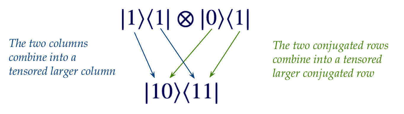
- This expresses the tensored outer-product
\(\otr{1}{1} \otimes \otr{0}{1}\)
as an outer-product of 2-qubit basis vectors: \(\otr{10}{11}\).
In-Class Exercise 9:
Use the just-described approach above to write
\(\otr{0}{0} \otimes \otr{1}{0}\) as a single
outer-product using the 2-qubit basis vectors,
and then confirm your results by working through the matrix versions.
In-Class Exercise 10:
Compute the projector \(\otr{0,+}{0,+}\) in two
ways:
- Write out the column and row forms of \(\kt{0,+}\) and
then tensor.
- Tensor the smaller projectors using Proposition 4.5.
In-Class Exercise 11:
Compute the matrix resulting from adding the operators
\(\otr{0}{1} + \otr{1}{0}\) and apply that to \(\kt{1}\).
4.8
Some important operators and their outer-product form
Let's start familiarizing ourselves with
some important unitary operators that form the foundation
for building quantum computing circuits.
First, let's look at the outer-product form for single qubit operators:
- We'll start with the simplest operator, the identity:
- Of course, we're used to writing
$$
I \eql \mat{1 & 0\\ 0 & 1}
$$
- But it can also be written in outer-product form as:
$$
I \eql \otr{0}{0} + \otr{1}{1}
$$
because
$$\eqb{
\otr{0}{0} + \otr{1}{1}
& \eql &
\mat{1 & 0}\mat{1\\ 0} + \mat{0 & 1}\mat{0\\ 1} \\
& \eql &
\mat{1 & 0\\ 0 & 0} + \mat{0 & 0\\ 0 & 1} \\
& \eql &
\mat{1 & 0\\ 0 & 1} \\
}$$
- We've seen that the "flip" operator \(X\) can be written
as
$$\eqb{
X & \eql & \otr{0}{1} + \otr{1}{0} \\
& \eql &
\mat{0 & 1\\ 0 & 0} + \mat{0 & 0\\ 1 & 0} \\
& \eql &
\mat{0 & 1\\ 1 & 0}
}$$
- Note:
- An outer-product is written in terms of vectors
\(\rhd\)
It's an outer-product of vectors.
- The vectors used are orthonormal basis vectors
\(\rhd\)
This way, algebraic expressions simplify through inner-products
of basis vectors.
- Typically, we use the standard basis vectors, in the examples here.
- The advantage of using the outer-product form is that
expressions can be simplified without expansion into a full-blown matrix.
- Example: let's see how this works with \(X\):
$$\eqb{
X\kt{0} & \eql & \parenl{\otr{0}{1} + \otr{1}{0}} \kt{0}
& \mbx{Substitute outer product form} \\
& \eql & \otr{0}{1}\kt{0} + \otr{1}{0}\kt{0}
& \mbx{Distribution} \\
& \eql & \kt{0}\, \parenl{\inr{1}{0}} + \kt{1}\, \parenl{\inr{0}{0}}
& \mbx{Associativity} \\
& \eql & \kt{1}
& \mbx{Exploit orthonormal inner products} \\
}$$
- The outer-product form is designed to exploit the
simplifications obtained from pairing orthonormal basis vectors
in inner products.
- Example:
$$\eqb{
X \, \parenl{ \alpha\kt{0} + \beta\kt{1} }
& \eql &
\parenl{\otr{0}{1} + \otr{1}{0}} \parenl{ \alpha\kt{0} + \beta\kt{1} }
& \mbx{Look for cases where inner-product = 1} \\
& \eql &
\kt{0} \parenl{\beta\inr{1}{1}} + \kt{1} \parenl{\alpha\inr{0}{0}}
& \mbx{The other two are 0 from orthogonality} \\
& \eql &
\beta\kt{0} + \alpha\kt{1}
&
}$$
Now let's look at a few important operators, along with their Dirac forms.
The four Pauli operators:
$$\eqb{
I & \eql & \otr{0}{0} + \otr{1}{1} & \eql & \mat{1 & 0\\0 & 1} \\
X & \eql & \otr{0}{1} + \otr{1}{0} & \eql & \mat{0 & 1\\1 & 0} \\
Y & \eql & -i\otr{0}{1} + i\otr{1}{0} & \eql & \mat{0 & -i\\i & 0} \\
Z & \eql & \otr{0}{0} - \otr{1}{1} & \eql & \mat{1 & 0\\0 & -1} \\
}$$
- These are useful in quantum computing, and essential to
quantum mechanics.
- Note: in quantum computing, the \(Y\) operator
is sometimes simplified to
$$
Y \eql -\otr{1}{0} + \otr{0}{1} \eql \mat{0 & 1\\-1 & 0}
$$
- The Z operator results in change of relative phase:
$$\eqb{
Z \parenl{ \alpha\kt{0} + \beta\kt{1} }
& \eql & \parenl{ \otr{0}{0} - \otr{1}{1} } \parenl{
\alpha\kt{0} + \beta\kt{1} } \\
& \eql &
\alpha\kt{0} - \beta\kt{1} \\
& \eql &
\alpha\kt{0} + e^{i\pi} \beta\kt{1} \\
}$$
Note:
- Recall that a unit-magnitude constant multiplying into a
qubit state does not change the state, as in
$$
e^{i\theta} (\alpha\kt{0} + \beta\kt{1})
\;\;\;\;\;\; \mbox{ is the same state as } \;\;\;\;\;\;
\alpha\kt{0} + \beta\kt{1}
$$
- But
$$
e^{i\theta} \alpha\kt{0} + \beta\kt{1}
\;\;\;\;\;\; \mbox{ is different from } \;\;\;\;\;\;
\alpha\kt{0} + \beta\kt{1}
$$
and different from \(\alpha\kt{0} + e^{i\theta} \beta\kt{1}\).
- Sometimes the notation
$$
\sigma_I = I
\;\;\;\;\;\;\;
\sigma_X = X
\;\;\;\;\;\;\;
\sigma_Y = Y
\;\;\;\;\;\;\;
\sigma_Z = Z
$$
is used.
- Properties:
- The Pauli operators are both Hermitian and unitary.
- Which means \(X^2 = Y^2 = Z^2 = I\).
(Repeating returns a qubit to its original state.)
- Wolfgang Pauli was one of the first generation key
contributors to the theory of quantum mechanics.
(The others: Planck, Einstein, Heisenberg, Schrodinger, Born,
Dirac, Bohr.)
The Hadamard operator \(H\):
- \(H\) is one of the most important operators in quantum computing.
- In both forms:
$$\eqb{
H & \eql &
\isqt{1} \parenl{ \otr{0}{0} + \otr{1}{0} + \otr{0}{1} - \otr{1}{1} }\\
& \eql &
\isqt{1} \mat{1 & 1\\ 1 & -1} \\
& \eql &
\mat{ \isqt{1} & \isqt{1}\\ \isqt{1} & -\isqt{1} }
}$$
- Again, we can see how the outer-product simplifies application:
$$\eqb{
H \kt{0} & \eql &
\isqt{1} \parenl{ \otr{0}{0} + \otr{1}{0} + \otr{0}{1} - \otr{1}{1} }
\kt{0} \\
& \eql & \isqt{1} \parenl{ \kt{0} + \kt{1} } \\
& \eql & \kt{+}
}$$
- A relationship between \(H\) and the Pauli operators:
$$\eqb{
H & \eql &
\isqt{1} \parenl{ \otr{0}{0} + \otr{1}{0} + \otr{0}{1} - \otr{1}{1} }\\
& \eql &
\isqt{1} \parenl{ (\otr{0}{1} + \otr{1}{0}) + (\otr{0}{0} - \otr{1}{1}) }\\
& \eql &
\isqt{1} \parenl{ X + Z }
}$$
In-Class Exercise 12:
Use both the outer-product and regular matrix approaches
to show \(Z = HXH\).
The outer-product form for 2-qubit operators:
- A 2-qubit operator in matrix form is a \(4\times 4\) matrix.
- Any outer-product of two standard basis vectors gives
us a matrix with a single \(1\), the rest \(0\)'s:
- Any outer-product of a standard basis vector with itself gives
a \(1\) on the diagonal.
- Example:
$$
\otr{10}{10}
\eql
\mat{0 \\ 0 \\ 1 \\ 0}
\mat{0 & 0 & 1 & 0}
\eql
\mat{0 & 0 & 0 & 0\\
0 & 0 & 0 & 0\\
0 & 0 & 1 & 0\\
0 & 0 & 0 & 0}
$$
- A matrix with \(1\) in an off-diagonal location (\(0\)'s elsewhere)
can also be written as an outer-product.
- Example:
$$
\mat{0 & 0 & 0 & 0\\
0 & 0 & 0 & 0\\
0 & 0 & 0 & 1\\
0 & 0 & 0 & 0}
\eql
\mat{0 \\ 0 \\ 1 \\ 0}
\mat{0 & 0 & 0 & 1}
\eql
\otr{10}{11}
$$
- Then, any \(4\times 4\) matrix with \(0\)'s and \(1\)'s can be written
as a sum of such outer-products.
- Example:
$$
I \eql \otr{00}{00} + \otr{01}{01} + \otr{10}{10} + \otr{11}{11}
$$
The \(\cnot\) operator:
4.9
A few special bases
A few bases tend to get used more often than others in quantum
computing:
- The standard basis (single and multiple qubits)
- The Hadamard basis (single and multiple qubits)
- The Bell basis (two qubits)
When does a basis matter?
- There are three cases when the choice of basis matters.
- First, and most importantly:
when measurement occurs, the measuring device always
has an associated basis.
- Thus, for example, if one measures in the Hadamard basis:
- The single-qubit Hadamard basis has: \(\kt{+}, \kt{-}\).
- Then, a qubit state is expressed in this basis:
$$
\psi \eql \alpha \kt{+} + \beta \kt{-}
$$
- After which, we know that an actual measurement will result in:
$$\eqb{
\kt{+} & \;\;\;\;\;\; & \mbox{ with probability } \magsq{\alpha}\\
\kt{-} & \;\;\;\;\;\; & \mbox{ with probability } \magsq{\beta}\\
}$$
- If we measured in Hadamard but expressed in standard, we'd
have to convert to Hadamard to assess probabilities, for example:
- Suppose
$$
\ksi \eql \smm{\frac{\sqrt{2}}{\sqrt{3}}} \kt{0}
+ \smm{\frac{1}{\sqrt{3}}} \kt{1}
$$
- Converting to Hadamard, we see that
$$
\ksi \eql \smm{\frac{\sqrt{2}+1}{\sqrt{6}}} \kt{+}
\; + \; \smm{\frac{\sqrt{2}-1}{\sqrt{6}}} \kt{-}
$$
- Thus, the probabilities associated with measurement outcomes are:
$$\eqb{
\mbox{Observe }\kt{+} & \;\;\;\;\;\;
\mbox{with probability } \smm{\magsq{ \frac{\sqrt{2}+1}{\sqrt{6}} }}\\
\mbox{Observe }\kt{-} & \;\;\;\;\;\;
\mbox{with probability } \smm{\magsq{ \frac{\sqrt{2}-1}{\sqrt{6}} }}\\
}$$
- Alternatively, using the projector approach we could:
- (Step 1) Identify the projectors \(\otr{+}{+}, \otr{-}{-}\)
- (Step 2) Apply each projector. For example, applying \(\otr{+}{+}\):
$$\eqb{
\otr{+}{+} \ksi
& \eql & \inr{+}{\psi} \: \kt{+} \\
& \eql &
\inrh{ \isqts{1}\br{0} + \isqts{1}\br{1}}{
\smm{\frac{\sqrt{2}}{\sqrt{3}}} \kt{0}
+ \smm{\frac{1}{\sqrt{3}}} \kt{1}}
\: \kt{+} \\
& \eql & \smm{\frac{\sqrt{2}+1}{\sqrt{6}}} \kt{+}
}$$
(The same can be done for \(\otr{-}{-}\))
- (Step 3) Compute the projected vector lengths to give
probabilities, for example:
$$
\magsq{ \smm{\frac{\sqrt{2}+1}{\sqrt{6}}} \kt{+} }
\eql
\magsq{ \smm{\frac{\sqrt{2}+1}{\sqrt{6}}} }
$$
(Similarly, the other probability is \(\magsq{ \frac{\sqrt{2}-1}{\sqrt{6}} }\))
- (Step 4) Normalize the projected vectors to give the outcomes,
for example: \(\kt{+}\)
(The other measurement outcome is of course \(\kt{-}\))
- The second case is when one is analyzing a Hermitian:
- Recall: a Hermitian packages projectors.
- And a tensored Hermitian does this across multiple qubits.
- Analysis is always easier when a Hermitian is expressed
in the coordinates of its eigenvector basis.
- In this case, the Hermitian is a diagonal matrix (eigenvalues
on the diagonal).
- We don't see much of this analysis in quantum computing but
it's heavily used in quantum mechanics.
- The third instance where a basis matters is when the vectors
in the basis serve a special purpose.
\(\rhd\)
This is the case with the Bell basis, as we'll see.
The standard basis
- For a single qubit, the standard basis is:
$$
\kt{0} \;\;\;\;\;\; \kt{1}
$$
- For two qubits:
$$
\kt{00},
\;\;\;\;\;\;
\kt{01},
\;\;\;\;\;\;
\kt{10},
\;\;\;\;\;\;
\kt{11}
$$
- For three qubits:
$$
\kt{000}, \;\;\;\;
\kt{001}, \;\;\;\;
\kt{010}, \;\;\;\;
\kt{011}, \;\;\;\;
\kt{100}, \;\;\;\;
\kt{101}, \;\;\;\;
\kt{110}, \;\;\;\;
\kt{111}
$$
- For n-qubits, it's the \(2^n\) vectors
$$
\kt{00\ldots 0},
\;\;\;\;\;\;
\kt{00\ldots 1},
\;\;\;\;\;\;
\ldots
\;\;\;\;\;\;
\kt{11\ldots 1}
$$
- The standard basis is the most commonly used basis
in quantum computing:
- Most states are expressed in this basis.
- And most measurements occur in this basis.
- Decimal shorthand notation:
- The binary strings are interpreted as decimal numbers.
- Thus, the 2-qubit basis is also written as:
\(\kt{0}, \kt{1}, \kt{2}, \kt{3}\)
- The n-qubit:
\(\kt{0}, \kt{1}, \ldots, \kt{2^n-1}\)
- Thus, the 3-qubit basis is written in these two ways:
$$\eqb{
\kt{0} & \eql & \kt{000} \\
\kt{1} & \eql & \kt{001} \\
\kt{2} & \eql & \kt{010} \\
\kt{3} & \eql & \kt{011} \\
\kt{4} & \eql & \kt{100} \\
\kt{5} & \eql & \kt{101} \\
\kt{6} & \eql & \kt{110} \\
\kt{7} & \eql & \kt{111}
}$$
- The decimal shorthand is very useful algebraically, for
example:
$$\eqb{
\ksi & \eql & \smf{1}{2} \parenl{ \kt{00} + \kt{01} + \kt{10} + \kt{11}} \\
& \eql & \smf{1}{2} \parenl{ \kt{0} + \kt{1} + \kt{2} + \kt{3} }\\
& \eql & \smf{1}{2} \sum_{k=0}^3 \kt{k}
}$$
- Notice that the above vector is an equal-coefficient superposition
$$\eqb{
\smf{1}{2} \sum_{k=0}^3 \kt{k}
& \eql &
\smf{1}{\sqrt{4}} \parenl{ \kt{0} + \kt{1} + \kt{2} + \kt{3} }\\
& \eql &
\smf{1}{\sqrt{2^2}} \kt{0} \: + \: \smf{1}{\sqrt{2^2}}\kt{1}
\: + \: \smf{1}{\sqrt{2^2}}\kt{2} \: + \: \smf{1}{\sqrt{2^2}} \kt{3}
}$$
- For \(3\) qubits this becomes
$$
\smf{1}{\sqrt{8}} \parenl{ \kt{0} + \kt{1} + \ldots + \kt{7} }
\eql
\smf{1}{\sqrt{2^3}} \sum_{k=0}^{2^3 - 1} \kt{k}
$$
- We will often see the n-qubit equal-superposition written as:
$$
\smf{1}{\sqrt{2^n}} \sum_{k=0}^{2^n-1} \kt{k}
$$
Or as
$$
\smf{1}{\sqrt{N}} \sum_{k=0}^{N-1} \kt{k}
$$
where \(N = 2^n\).
The Hadamard basis:
- This is typically used in the single-qubit case for measurement.
- The two basis vectors: \(\kt{+}, \kt{-}\)
- These vectors themselves can of course be expressed in
the standard basis:
$$\eqb{
\kt{+} & \eql & \isqts{1} (\kt{0} + \kt{1}) \\
\kt{-} & \eql & \isqts{1} (\kt{0} - \kt{1}) \\
}$$
- We saw one example: polarization.
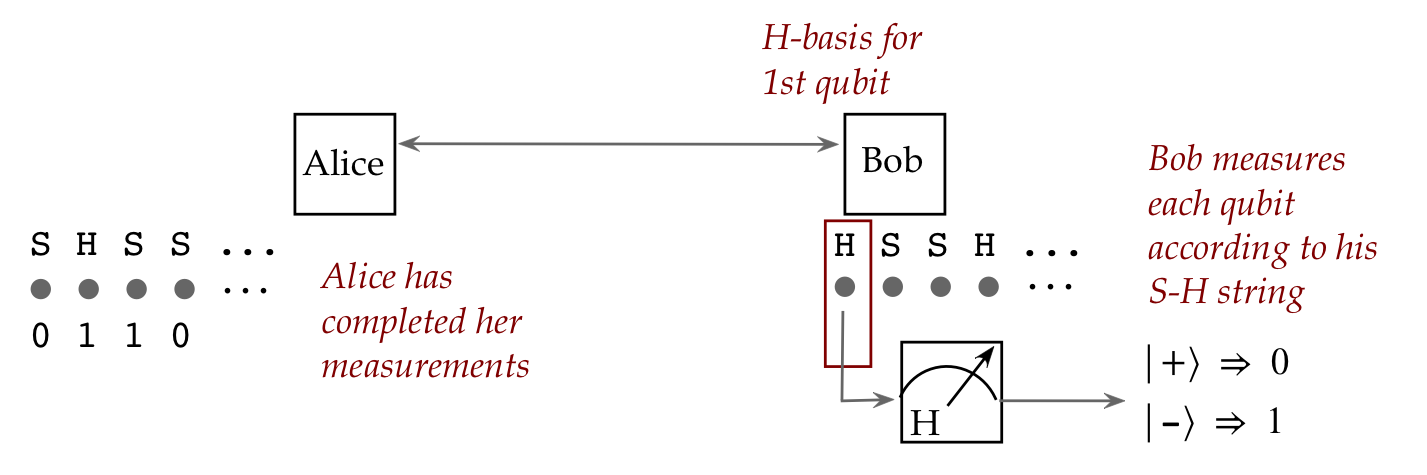
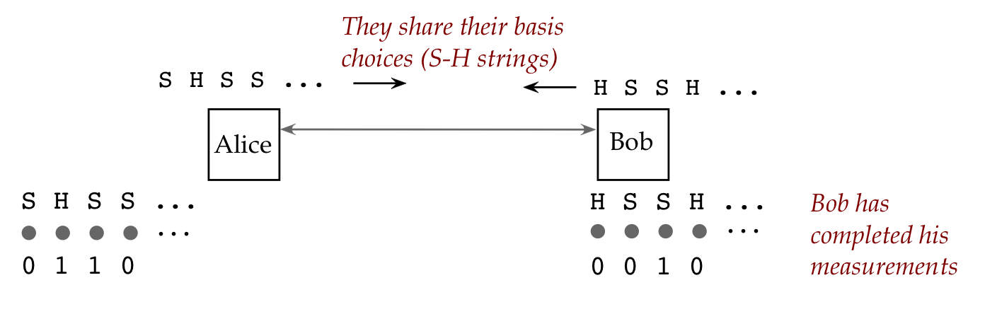
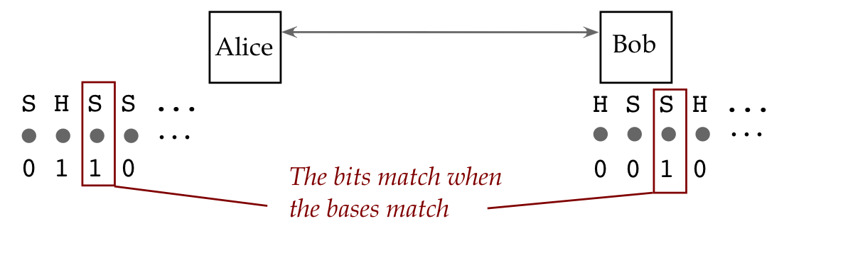
- And we saw its use in the BB-84 key-distribution protocol.
- The Hadamard unitary operator, on the other hand,
is often used in the multiple-qubit case where it is tensored.
The Bell basis:
- This is a 2-qubit basis with the following four vectors:
$$\eqb{
\kt{\Phi^+} & \eql & \isqts{1} \parenl{ \kt{00} + \kt{11} } \\
\kt{\Phi^-} & \eql & \isqts{1} \parenl{ \kt{00} - \kt{11} } \\
\kt{\Psi^+} & \eql & \isqts{1} \parenl{ \kt{01} + \kt{10} } \\
\kt{\Psi^-} & \eql & \isqts{1} \parenl{ \kt{01} - \kt{10} } \\
}$$
- Sometimes these are also named
\(\beta_{00}, \beta_{01}, \beta_{10}, \beta_{11}\).
(We'll use the former.)
- This basis is not really used for measurement but instead,
one or more of these vectors are used as a desirable state to
initiate a computation, as we'll see below.
In-Class Exercise 13:
Show that the four Bell vectors do in fact form a basis
for the 2-qubit vector space.
4.10
Entanglement: a first look
Consider the first Bell vector:
$$
\kt{\Phi^+} \eql \isqts{1} \parenl{ \kt{00} + \kt{11} }
$$
- This is a 2-qubit state.
- Let's ask: are there two 1-qubit states
\(\kt{v}\) and \(\kt{w}\) such that
$$
\kt{\Phi^+} \eql \kt{v} \otimes \kt{w}?
$$
- Let
$$\eqb{
\kt{v} & \eql & \alpha_0 \kt{0} + \alpha_1 \kt{1} \\
\kt{w} & \eql & \beta_0 \kt{0} + \beta_1 \kt{1} \\
}$$
- Then,
$$\eqb{
\kt{v} \otimes \kt{w}
& \eql &
\parenl{ \alpha_0 \kt{0} + \alpha_1 \kt{1} }
\otimes
\parenl{ \beta_0 \kt{0} + \beta_1 \kt{1} } \\
& \eql &
\alpha_0\beta_0 (\kt{0} \otimes \kt{0})
\plss
\alpha_0\beta_1 (\kt{0} \otimes \kt{1})
\plss
\alpha_1\beta_0 (\kt{1} \otimes \kt{0})
\plss
\alpha_1\beta_1 (\kt{1} \otimes \kt{1})\\
& \eql &
\alpha_0\beta_0 \kt{00}
\plss
\alpha_0\beta_1 \kt{01}
\plss
\alpha_1\beta_0 \kt{10}
\plss
\alpha_1\beta_1 \kt{11}
}$$
- Now equate this to \(\kt{\Phi^+}\):
$$
\alpha_0\beta_0 \kt{00}
+
\alpha_0\beta_1 \kt{01}
+
\alpha_1\beta_0 \kt{10}
+
\alpha_1\beta_1 \kt{11}
\eql
\isqts{1} \parenl{ \kt{00} + \kt{11} }
$$
- Notice that the existence of \(\kt{00}\) implies
\(\alpha_0\) and \(\beta_0\) are both nonzero.
- Similarly \(\kt{11}\) implies
\(\alpha_1\) and \(\beta_1\) are both nonzero.
- This would force inclusion of \(\kt{01}\) and \(\kt{10}\)
on the left.
- Thus, no tensoring of 1-qubit vectors can equal \(\kt{\Phi^+}\).
- Yet \(\kt{\Phi^+}\) is a valid 2-qubit state because it's
a linear combination of 2-qubit basis vectors:
$$
\kt{\Phi^+} \eql \isqts{1} \kt{00} + \isqts{1} \kt{11}
$$
What we've discovered is this:
- Let \(B_1\) be the basis vectors \(\kt{0}, \kt{1}\) for the
first qubit, and \(V_1\) be the vector space
$$
V_1 \eql \{ \alpha_0 \kt{0} + \alpha_1 \kt{1} \}
$$
That is, unit-length linear combinations of the basis vectors of
space \(V_1\).
- Let \(B_2\) and \(V_2\) be the corresponding basis, and
vector space for the 2nd qubit:
$$
V_2 \eql \{ \beta_0 \kt{0} + \beta_1 \kt{1} \}
$$
- We construct the 2-qubit vector space by first
putting together its basis \(B_{1,2}\) by tensoring the
basis vectors from \(V_1\) and \(V_2\):
$$\eqb{
B_{1,2} & \eql & \{
\kt{0} \otimes \kt{0}, \;
\kt{0} \otimes \kt{1}, \;
\kt{1} \otimes \kt{0}, \;
\kt{1} \otimes \kt{1},
\} \\
& \eql & \{
\kt{00}, \kt{01}, \kt{10}, \kt{11}
\}
}$$
- Then, the vectors in the space \(V_1 \otimes V_2\)
are linear combinations of these basis vectors:
$$
V_1 \otimes V_2
\eql
\setl{
a_{00} \kt{00} + a_{01} \kt{01} + a_{10} \kt{10} + a_{11} \kt{11}
}
$$
- Now, there are vectors in \(V_1 \otimes V_2\) that
can be expressed as tensors of smaller vectors, one each in
\(V_1\) and \(V_2\), for example:
- Let \(\kt{0}\) be an example vector from \(V_1\) (1st qubit).
- Let
$$
\smf{\sqrt{2}}{\sqrt{3}} \kt{0} + \smf{1}{\sqrt{3}} \kt{1}
$$
be a vector from \(V_2\).
- Now,
$$
\ksi \eql \smf{\sqrt{2}}{\sqrt{3}} \kt{00} + \smf{1}{\sqrt{3}} \kt{01}
$$
is a vector in \(V_1 \otimes V_2\) because it's a linear
combination of basis vectors.
- And yet it's expressible as a tensor of the smaller vectors:
$$\eqb{
\kt{0} \otimes \parenl{ \smf{\sqrt{2}}{\sqrt{3}} \kt{0} +
\smf{1}{\sqrt{3}} \kt{1} }
& \eql &
\smf{\sqrt{2}}{\sqrt{3}} (\kt{0} \otimes \kt{0}) +
\smf{1}{\sqrt{3}} (\kt{0} \otimes \kt{1}) \\
& \eql &
\smf{\sqrt{2}}{\sqrt{3}} \kt{00} +
\smf{1}{\sqrt{3}} \kt{01} \\
& \eql & \ksi
}$$
- At the same time, there are vectors \(\kt{w}\) in
\(V_1 \otimes V_2\) that cannot be expressed as tensored
smaller vectors:
$$
\kt{w} \neq \kt{v_1} \otimes \kt{v_2}
$$
for any \(\kt{v_1}\in V_1, \kt{v_2}\in V_2\).
\(\rhd\)
Example: \(\kt{w} = \kt{\Phi^+} = \isqt{1} \kt{00} + \isqt{1} \kt{11} \)
- Definitions:
- A vector like \(\kt{\Phi^+}\) that cannot be expressed
by tensoring smaller vectors is called an entangled vector.
- A vector like \(\ksi\) that can be expressed as such
is called a separable vector.
- The term entanglement refers both to:
- The phenomenon, as described above.
- Physical implementations where two qubits are deliberately
set up so that the combined 2-qubit state is entangled.
How do we know whether a 2-qubit state is entangled?
- That is, given a generic 2-qubit state
$$
\ksi \eql a_{00} \kt{00} + a_{01} \kt{01} + a_{10} \kt{10} + a_{11} \kt{11}
$$
we want to know if it's entangled.
- If it were separable (not-entangled),
we'd be able to find two vectors \(\kt{v}, \kt{w}\), whose tensor
would give us \(\ksi\):
$$
\ksi \eql \kt{v} \otimes \kt{w}
$$
- Let
$$\eqb{
\kt{v} & \eql & \alpha_0 \kt{0} + \alpha_1 \kt{1} \\
\kt{w} & \eql & \beta_0 \kt{0} + \beta_1 \kt{1}
}$$
represent two generic 1-qubit states.
- If we tensor them, the resulting 2-qubit vector is:
$$\eqb{
& \; &
\parenl{ \alpha_0 \kt{0} + \alpha_1 \kt{1} }
\otimes
\parenl{ \beta_0 \kt{0} + \beta_1 \kt{1} } \\
& \eql &
\alpha_0\beta_0 \kt{00}
\plss
\alpha_0\beta_1 \kt{01}
\plss
\alpha_1\beta_0 \kt{10}
\plss
\alpha_1\beta_1 \kt{11}
}$$
- And if this were to produce
$$
\ksi \eql a_{00} \kt{00} + a_{01} \kt{01} + a_{10} \kt{10} + a_{11} \kt{11}
$$
it must be that
$$\eqb{
\alpha_0\beta_0 & \eql & a_{00} \\
\alpha_0\beta_1 & \eql & a_{01} \\
\alpha_1\beta_0 & \eql & a_{10} \\
\alpha_1\beta_1 & \eql & a_{11} \\
}$$
From which we see that
$$\eqb{
a_{00} a_{11} & \eql & \alpha_0\beta_0 \alpha_1\beta_1 \\
a_{01} a_{10} & \eql & \alpha_0\beta_0 \alpha_1\beta_1 \\
}$$
And so, for separability:
$$
a_{00} a_{11} - a_{01} a_{10} \eql 0
$$
Which gives us a condition to test for (for the 2-qubit case).
- For example, with
$$
\kt{\Phi^+} \eql \isqts{1} \parenl{ \kt{00} + \kt{11} } \\
$$
we see that
$$
a_{00} a_{11} - a_{01} a_{10}
\eql \isqts{1} \isqts{1} - 0
\; \neq \; 0
$$
Which means \(\kt{\Phi^+}\) is not separable (and therefore entangled).
- Similarly, with
$$
\ksi \eql \isqts{1} \parenl{ \kt{00} + \kt{01} } \\
$$
we see that
$$
a_{00} a_{11} - a_{01} a_{10}
\eql \isqts{1}\: 0 \; - \; \isqts{1}\: 0
\eql 0
$$
Which makes \(\ksi\) separable. Intuitively, we see the
separabability as well:
$$
\isqts{1} \parenl{ \kt{00} + \kt{01} }
\eql \kt{0} \otimes \parenl{ \isqts{1}\kt{0} + \isqts{1}\kt{1} }
$$
-
See solved problems
for another example.
An aside about entanglement:
- Entanglement is a complicated sub-topic that is still
under active research.
- There exist tests of entanglement that generalize
to multiple qubits. We will not cover these in the course.
- Entanglement is a property of how tensoring is set up.
- Once we have a tensor product defined, an entangled
vector from the larger space is entangled no matter what bases are used.
- It is possible for a larger system to be constructed
by tensoring subsystems in different ways.
- Then, it's possible for a larger-system state to be
entangled with respect to one subsystem but not the other.
(See the Rieffel book for an example.)
- In this course, the tensor products we will see
won't have this issue.
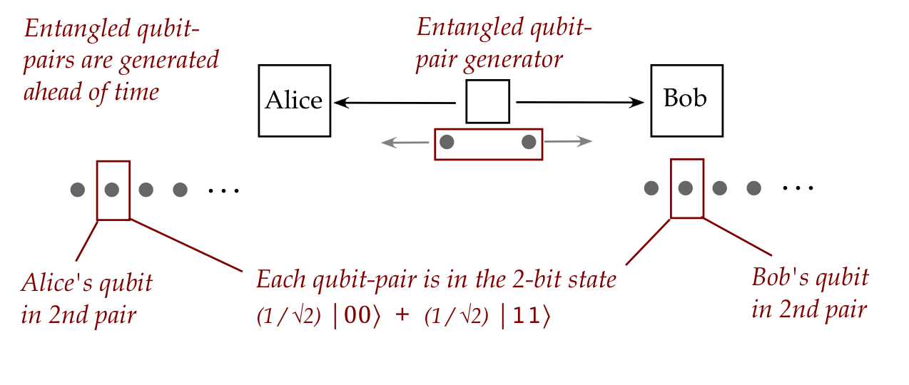
The most important (and weird) consequence of entanglement:
- Consider flying qubits.
- One can create a pair of such qubits in an entangled state:
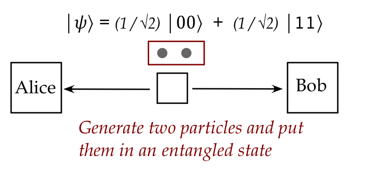
- Then, these qubits can be physically separated and sent in
different directions:
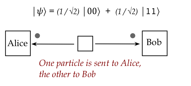
- What's truly astonishing:
- The two particles maintain their entangled state no matter
what the intervening distance.
- The implication:
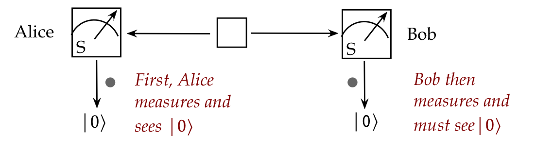
- If Alice measures her qubit and sees \(\kt{0}\),
then Bob's single-qubit measurement performed afterwards
will result in \(\kt{0}\)!
- Note:
- At the time of measurement, Alice won't know which outcome,
\(\kt{0}\) or \(\kt{1}\), will appear.
- But whichever outcome appears, Bob will see the same
even if his measurement occurs much later.
- This is what Einstein termed "spooky action at a distance".
- We will later undertake a more careful analysis of how
entangled particles might have this property:
- Instead of explaining away this property in a straightforward
way, the analysis will only deepen the mystery.
- A pair of entangled particles is sometimes called an EPR
pair, after Einstein-Podolsky-Rosen, whose 1935 paper first
raised the possibility of entangled pairs and "spooky action"
as a way to question whether quantum mechanics was complete.
4.11
The E91 key distribution protocol: a first glimpse
Recall the goal of key distribution:
- Alice and Bob want to create a shared secret key for future
communications.
- This secret key is a (classical) random binary string
like 10100111010101101 ... (long enough, for high security).
- Then, future text messages use the same key to encrypt (on one
side), and decrypt (on the other).
- The actual encryption mechanism can use the key in different
ways.
\(\rhd\)
For example: apply XOR using the key to a binary text message.
- Recall from BB84:
- BB84 has Alice create and send qubits to Bob.
- After that, they apply measurements in different bases.
- Then, they compare basis-choices afterwards, and
when in agreement, use the corresponding qubits.
Note: Eve can intercept the qubits to try and attack.
- The E91 protocol is named after Artur Ekert, who published this
idea in 1991.
- What's interesting:
- No qubits are exchanged.
\(\rhd\)
Eve has nothing to work with!
The E91 protocol:
The protocol relies on what happens when measuring an
entangled pair:
- Let's focus on the cases where their bases match.
- Consider when Alice measures with S-basis:
- Suppose the outcome is \(\kt{0}\).
- Then, Bob's outcome is also \(\kt{0}\) (with certainty).
- This is easy to see with the entangled state:
$$
\kt{\Phi^+} \eql \isqts{1} \parenl{ \kt{00} + \kt{11} }
$$
- If Alice sees \(\kt{0}\), the combined 2-qubit state
is:
$$
\kt{00} \eql \kt{0} \otimes \kt{0}
$$
which means Bob's qubit must be measured as \(\kt{0}\).
- We can summarize this as: when both use the S-basis in
sequence, both interpretations match:
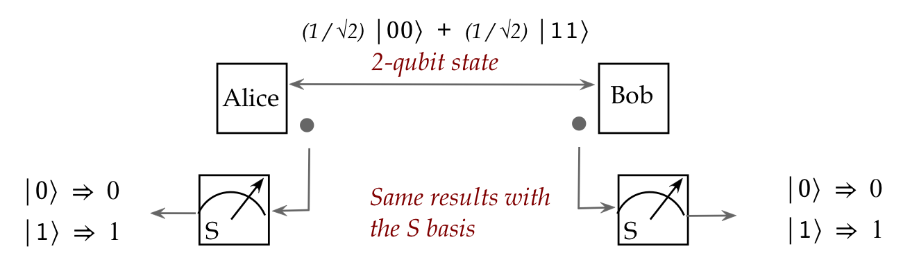
- What is less clear at the moment is that the same
holds with the H-basis:
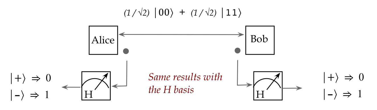
- When Alice uses the H-basis and sees \(\kt{+}\) the
outcome state turns out to be:
$$
\kt{+} \otimes \kt{+}
$$
(We will later see why this is the outcome.)
- Thus, Bob's H-basis measurement leads to the same outcome.
- When we learn about how 2-qubit measurement works, we'll
re-examine this part.
- We will also see why we developed the (more complicated)
theory of projectors.
What can Eve do?
- We assume that the classical channel is secure (perhaps using
a previously generated key).
- Alice and Bob do not communicate qubits
\(\rhd\)
There is nothing for Eve to intercept.
- However, Eve could have tampered with the earlier
generation of entangled pairs.
- As in BB84, Alice and Bob can sacrifice some key bits to
test whether the pairs are properly entangled.
- They perform measurements to see if the results match what
entanglement predicts.
Practicalities:
- The really hard part, in practice, is storing entangled qubits.
- There is active on-going research in photon storage.
- Other approaches seek to entangle a flying qubit with
a stationary qubit, so that stationary qubits can maintain entangled state.
4.12
Matrix exponentials and fractional powers
Recall how we defined the exponential of a complex number:
- The rules of addition and multiplication for real numbers
were extended to complex numbers in a straightforward way.
(See Module 2.)
- But it was not obvious how one exponentiates a complex number
\(z\) to calculate \(e^z\).
- The way forward came about by looking at the Taylor
series expansion for the real function \(e^x\)
$$
e^x \eql
1 + x + \frac{x^2}{2!} + \frac{x^3}{3!} + \ldots
$$
The right side has only arithmetic operations.
- From this, we defined the complex exponential
$$
e^z \;\; \defn \;\;
1 + z + \frac{z^2}{2!} + \frac{z^3}{3!} + \ldots
$$
which eventually led to Euler's relation:
$$
e^{i\theta} \eql
\cos\theta + i \sin\theta
$$
The same approach can be used to define matrix
exponentiation:
- First, let's ask: what arithmetic operations
do we already have with matrices?
Answer:
- We have addition \(A+B\) for matrices \(A, B\).
- We have multiplication \(AB\).
- Scalar multiplication \(\alpha A\)
- From this follows powers of a matrix:
$$
A^k \eql AA \ldots A \;\;\;\;\;\;\;\mbox{ (multiplication \(k\) times)}
$$
- Then, for a matrix \(A\), define
$$
e^A \;\; \defn \;\;
I + A + \frac{A^2}{2!} + \frac{A^3}{3!} + \ldots
$$
The right side uses operations that already exist and so,
if the infinite series converges, we have a working definition.
- It can be shown (not easily) that the infinite series does converge
for complex-valued matrices.
- Two forms of the matrix exponential are commonly used:
- The direct form, as above.
- With an additional scalar variable
$$
e^{\alpha A} \;\; \defn \;\;
I + \alpha A + \frac{\alpha^2 A^2}{2!}
+ \frac{\alpha^3 A^3}{3!} + \ldots
$$
- When the scalar is \(\alpha = i\), we get the complex
matrix exponential \(e^{iA}\)
- This is useful in quantum computing because, if \(A\)
is Hermitian, then \(e^{iA}\) is unitary because
$$
\left( e^{iA} \right)^\dagger e^{iA}
\eql
e^{-iA^\dagger} e^{iA}
\eql
e^{-iA} e^{iA}
\eql
I
$$
Note:
- It's true but not obvious that
\(\left( e^{iA} \right)^\dagger = e^{-iA^\dagger}\).
- In the last part, we get \(e^{i(A-A)}\) where
the exponent is not the number zero, but the zero-matrix.
- In particular, the four Pauli operators \(I, X, Y, Z\) are
Hermitian:
- Then, \(e^{iI}, e^{iX}, e^{iY}, e^{iZ}\) are all unitary matrices.
- Some of these are useful in practice.
We'll merely list a bunch of properties without proof:
- If \(D\) is a (square) diagonal matrix with diagonal entries
\(d_1,\ldots, d_n\), then
$$
e^D \eql
\mat{
e^{d_1} & 0 & 0 & 0\\
0 & e^{d_2} & 0 & 0 & \\
0 & 0 & \ddots & 0\\
0 & 0 & 0 & e^{d_n}
}
$$
- If \(A\) can be written as \(A=S D S^{-1}\) where
\(D\) is diagonal and \(S\) is some matrix with an inverse,
then
$$
e^{S D S^{-1}} \eql S e^D S^{-1}
$$
- \( \left( e^{A} \right)^T = e^{A^T} \)
- \(e^{(z_1 + z_2)A} = e^{z_1A} e^{z_2A}\) for complex
numbers \(z_1, z_2\).
- If \(AB = BA\) then \(e^{A}e^{B} = e^{A+B}\).
- A result that will be useful in quantum computing:
- If \(A^2=I\) then
$$\eqb{
e^{i\theta A}
& \eql &
I + (i\theta) A + (i\theta)^2 \frac{A^2}{2!}
+ (i\theta)^3 \frac{A^3}{3!} + \ldots \\
& \eql &
\parenl{ I - \theta^2 A^2 + \theta^4 A^4 \ldots }
+
\parenl{i\theta A - i^3\theta^3 A^3 + i^5\theta^5 A^5 \ldots } \\
& \eql &
\parenl{ I - \theta^2 I + \theta^4 I \ldots }
+
\parenl{i\theta A - i\theta^3 A^2A + i\theta^5 A^4 A \ldots } \\
& \eql &
\parenl{ 1 - \theta^2 + \theta^4 \ldots }I
+
\parenl{\theta - \theta^3 + \theta^5 \ldots }iA \\
& \eql &
I\cos\theta + iA\sin\theta
}$$
Fractional powers:
- We know how positive integral powers like \(A^k\) work.
- But what about \(A^{\frac{1}{2}}\) or \(A^{\frac{1}{n}}\)
for integer \(n\)?
- The definition is easy:
\(X=A^{\frac{1}{n}}\) if \(X^n = A\).
- But computing such fractional powers is complicated.
- And it isn't clear how many n-th roots exist.
- For example,
$$
\mat{a & b\\ c & -a}^2
\eql
\mat{a^2+bc & 0\\ 0 & a^2+bc}
$$
Which means for any values of \(a,b,c\) such that \(a^2+bc=1\),
the matrix
$$
\mat{a & b\\ c & -a}
\eql
\mat{1 & 0\\ 0 & 1}^{\frac{1}{2}}
$$
Thus, \(I\) has an infinite number of square roots!
- If \(A\) is Hermitian then it can be written as
(Recall: the spectral theorem):
$$
A \eql S D S^{-1}
$$
Then
$$
(S D^{\frac{1}{2}} S^{-1})^2 \eql A
$$
Which means any combination of real-valued diagonal square roots
elements of \(D\) will be a square root of \(A\).
\(\rhd\)
\(A\) has \(2^n\) square roots of the form \(S D^{\frac{1}{2}} S^{-1}\)
4.13*
Aside: commutators, direct sums
We will occasionally use these asides to point out terminology
and concepts that are related but not directly required
for quantum computing.
About commutators:
- We know that matrix multiplication is not commutative,
i.e., in general
$$
A B \; \neq \; B A
$$
- One useful quantification of "how non-commutative" for two
operators \(A\) and \(B\) is the so-called commutator
$$
[A, B] \; \defn \; AB - BA
$$
- Then, clearly, A commutes with B if \([A,B] = 0\).
- One powerful result is that if \([A,B] = 0\),
one can find a common eigenbasis for both \(A\) and \(B\).
- In this case, when \(A\) and \(B\) are measurement
operators, the outcomes of measurement are the same.
- Then, measurement with \(A\) produces predictable outcomes
with \(B\).
- Thus, Heisenberg uncertainty is not present (or zero) for
commuting measurement operators.
- When \([A,B] \neq 0\) Heisenberg's uncertainty principle can
be quantified in terms of a lower bound featuring the commutator \([A,B]\).
Direct sums:
- Just as the tensor product \(\otimes\) is a "sort of" product,
one could ask: is there an equivalent "sort of" sum?
- The answer: yes.
- We'll provide only a quick and dirty intuitive overview.
- Consider the two vectors
$$
\kt{v} \eql \mat{1 \\ 2 \\ 3}
\;\;\;\;\;\;\;\;
\kt{w} \eql \mat{4\\ 5}
$$
- Clearly, they are incompatible for regular addition, coming
from different vector spaces.
- However, one can expand both into
$$
\kt{v} \eql \mat{1 \\ 2 \\ 3\\ 0\\ 0}
\;\;\;\;\;\;\;\;
\kt{w} \eql \mat{0\\ 0\\ 0\\ 4\\ 5}
$$
- They are now addition-compatible
$$
\kt{v} \oplus \kt{w} \eql
\mat{1 \\ 2 \\ 3\\ 4\\ 5}
$$
- In this manner, one can construct the direct sum of
two differently-dimensioned vector spaces \(V\) and \(W\):
- Suppose \(V\) has basis vectors \(\kt{v_1},\ldots,\kt{v_m}\)
\(\rhd\)
Any vector \(v\in V\) has \(m\) elements
- Suppose \(W\) has basis vectors \(\kt{w_1},\ldots,\kt{w_n}\)
\(\rhd\)
Any vector \(w\in W\) has \(n\) elements
- We add trailing \(n\) trailing 0's to every \(v\in V\).
- And prefix \(m\) 0's to every \(w\in W\).
- Now all vectors have \(m+n\) elements.
- Then, a basis for the direct sum space
\(V\oplus W\) are the \(m+n\) vectors
$$
\kt{v_1},\ldots,\kt{v_m}, \kt{w_1},\ldots,\kt{w_n}
$$
- Where is this useful?
- Notice that orthonormal subspaces "direct sum" into the
original space.
- For example, with real vectors, let
$$\eqb{
V & \eql & \;\;\;\; \mbox{all vectors in the x-y plane} \\
W & \eql & \;\;\;\; \mbox{all vectors along z-axis} \\
}$$
Then \(V\oplus W\) is 3D space.
- When we look further into projective measurement, what we'll
see is that measurement outcomes divide into such direct-sum subspaces.
- Thus, the usefulness comes in providing a rigorous
mathematical foundation to measurement.
4.14*
Entanglement: a summary
Entanglement is indeed strange and often confusing.
Let's revisit and summarize entanglement with slightly different notation:
- Consider two qubits where
$$\eqb{
V & \eql & \setl{ \mbox{all possible 1st qubit states} } \\
W & \eql & \setl{ \mbox{all possible 2nd qubit states} } \\
}$$
- We now pick a basis for each, for example:
$$\eqb{
B_V & \eql & \setl{\kt{0}_V, \: \kt{1}_V} & \eql & \mbox{a basis for } V \\
B_W & \eql & \setl{\kt{0}_W, \: \kt{1}_W} & \eql & \mbox{a basis for } W \\
}$$
Here, we've picked the standard basis for each and deliberately
labeled the standard vectors to identify which qubit.
- Now tensor all possible pairs:
$$\eqb{
B_{V,W} & \eql &
\setl{
\kt{0}_V \otimes \kt{0}_W, \:
\kt{0}_V \otimes \kt{1}_W, \:
\kt{1}_V \otimes \kt{0}_W, \:
\kt{1}_V \otimes \kt{1}_W
}
& \mbx{Tensor one basis vector from \(V\) with one from \(W\)}\\
& \eql &
\setl{ \kt{00}, \: \kt{01}, \: \kt{10}, \: \kt{11} }
& \mbx{Short forms}
}$$
- Now consider two sets of vectors:
$$\eqb{
\Omega_{V,W} & \eql & \setl{ \kt{v}\otimes\kt{w}:
\kt{v}\in V, \kt{w}\in W}
& \mbx{All possible tensors of one vector in \(V\) and one in \(W\)}\\
\Omega_{V\otimes W} & \eql &
\mbox{span}\parenl{ \kt{00}, \: \kt{01}, \: \kt{10}, \: \kt{11} }
& \mbx{All possible linear combinations of \(B_{V,W}\) basis vectors}
}$$
- We now ask: are these two sets the same?
- First, note that \(\Omega_{V,W} \subseteq \Omega_{V\otimes W}\):
- We want to argue that any vector in \(\Omega_{V,W}\)
is in \(\Omega_{V\otimes W}\).
- Let
$$\eqb{
\kt{v} & \eql & \alpha\kt{0}_V + \beta\kt{1}_V \\
\kt{w} & \eql & \gamma\kt{0}_W + \delta\kt{1}_W \\
}$$
where we've added subscripts to clarify which basis.
- Then,
$$\eqb{
\kt{v} \otimes \kt{w} & \eql &
\parenl{ \alpha\kt{0}_V + \beta\kt{1}_V }
\otimes
\parenl{ \gamma\kt{0}_W + \delta\kt{1}_W } \\
& \eql &
\alpha\gamma\kt{00} + \alpha\delta\kt{01}
+ \beta\gamma{10} + \beta\delta\kt{11} \\
& \eql &
\mbox{a linear combination of vectors in } B_{V,W}\\
& \in &
\mbox{span}\parenl{ \kt{00}, \: \kt{01}, \: \kt{10}, \: \kt{11} }
}$$
- Which means
$$
\kt{v} \otimes \kt{w} \in \Omega_{V\otimes W}
$$
- Thus, any vector in \(\Omega_{V,W}\)
is in \(\Omega_{V\otimes W}\).
- Such vectors are called separable 2-qubit vectors.
- But
\(\Omega_{V,W} \neq \Omega_{V\otimes W}\):
- There are vectors in \(\Omega_{V\otimes W}\) not in
\(\Omega_{V,W}\)
- Example:
$$
\ksi \eql \isqts{1}\parenl{ \kt{00} + \kt{11} }
$$
- Clearly, this is a linear combination of the 2-qubit
basis vectors.
- But this \(\ksi\) cannot be written as
$$
\ksi \eql \kt{v} \otimes \kt{w}
$$
where \(\kt{v}\in V, \kt{w}\in W\).
- We showed this earlier: no tensor of vectors in
\(V\) and \(W\) produces \(\ksi\).
- Such a vector that's in the larger space \(\Omega_{V\otimes W}\)
but not in \(\Omega_{V,W}\) is entangled.
Could this entanglement be a result of our choice of basis?
- The answer: no
- Suppose instead we had picked bases
$$\eqb{
B^\prime_V & \eql & \setl{\kt{v_1}, \: \kt{v_2} }
& \eql & \mbox{a basis for } V \\
B^\prime_W & \eql & \setl{\kt{w_1}, \: \kt{w_2} }
& \eql & \mbox{a basis for } W \\
}$$
For example:
$$\eqb{
B^\prime_V & \eql & \setl{\kt{+}_V, \: \kt{-}_V} \\
B^\prime_W & \eql & \setl{
\smf{\sqrt{3}}{2}\kt{0}_W - \smf{1}{2}\kt{1}_W, \:
\smf{1}{2}\kt{0}_W + \smf{\sqrt{3}}{2}\kt{1}_W } \\
}$$
- Then, it turns out that tensoring all possible
combinations (four of them) results in the same span:
- Let
$$
B^\prime_{V,W}
\eql \setl{
\kt{v_1}\otimes\kt{w_1}, \:
\kt{v_1}\otimes\kt{w_2}, \:
\kt{v_2}\otimes\kt{w_1}, \:
\kt{v_2}\otimes\kt{w_2}
}
$$
- We could ask whether
$$
\mbox{span}\parenl{
\kt{v_1}\otimes\kt{w_1}, \:
\kt{v_1}\otimes\kt{w_2}, \:
\kt{v_2}\otimes\kt{w_1}, \:
\kt{v_2}\otimes\kt{w_2}
}
$$
is a different set than
$$
\mbox{span}\parenl{ \kt{00}, \: \kt{01}, \: \kt{10}, \: \kt{11} }
$$
- However, it's straightforward to show that
both are equal.
Can entangled states be created?
- We already know they cannot be created from 1-qubit
unitary operators:
- Suppose we have unitary operators \(A\) and \(B\)
for qubits \(1\) and \(2\).
- Then
$$
A\kt{v} \otimes B\kt{w} \eql
\parenl{A \otimes B} \parenl{ \kt{v} \otimes \kt{w} }
$$
- Thus, the 2-qubit operator \(C = A \otimes B\)
creates the separable state \(\kt{v} \otimes \kt{w}\)
- In other words, applying \(A\) and \(B\) does not
create an entangled state.
- Later, we will see how \(\cnot\) creates an entangled state.
A sketch of entanglement history:
- Soon after the development of early quantum mechanics in the 1920's,
Einstein and colleagues pointed out the difficulties with
entangled states.
- At this time, nobody knew for sure whether such states were
possible in nature.
- In the 1950's John Bell devised the theory for an experiment
that could prove or disprove.
- Such experiments began to be carried out in the 1970's,
culminating in careful experiments that eventually received the 2022
Nobel.
- These proved that entanglement exists in nature and can be
created in the lab.
- Meanwhile, in quantum computing, \(\cnot\) was realized
in hardware.
- And protocols were devised (E91) to exploit entanglement.
4.15
Summary
Between this module and the earlier Module 2, we have covered
a lot of new linear algebra:
- Complex numbers and vectors.
- The entirely new and somewhat strange Dirac notation.
- Unit-length simplification, phase equivalence.
- Important types of operators: projector, unitary, Hermitian.
- The sandwich.
- Tensors for vectors, tensors for operators.
- Some well-known bases.
- Entanglement, including an application of this strange phenomenon.
- Matrix exponentials and fractional powers.
Fortunately, this is all the linear algebra we need.
The Dirac notation does take acclimation, and that happens by
doing the (occasionally tedious) exercises, and trying out the
solved problems on your own.
Don't forget: Module-4 solved problems