Module objectives
By quantum linear algebra, we mean the linear
algebra needed for quantum computing.
This module's sole aim is to mathematically set us up for quantum
computing:
- Complex numbers and vectors.
- Dirac notation, which takes getting used to.
- Unit length simplification
- Projector, Hermitian and unitary matrices.
- Change-of-basis.
Some of this material might be a bit dry, but is necessary
before we get to the interesting stuff in later modules.
2.1
Why do we need the linear algebra of complex vectors?
We will over the course develop intuition for why we need
complex-number vectors and certain types of matrices.
And we will see mathematical reasons for why complex vectors
emerge from simple observations and basic assumptions.
For now, we'll provide a high-level operational view as
motivation.
Let's start by recalling how a standard electronic circuit
(in a calculator or computer) performs an arithmetic operation:
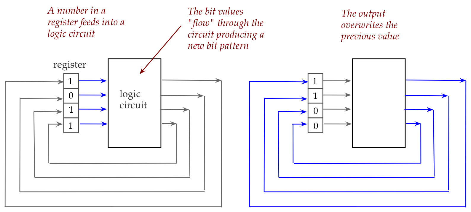
- Here, a binary number sits in a device (called a register) that
holds bits (the number's digits).
- These bits then flow into a logic circuit, which we've seen
earlier consists of a collection of Boolean gates (like AND, OR and
NOT gates).
- The gates together achieve the desired computation (increment,
in the above example), and the resulting number is fed back into the
register.
- This conceptual description is reasonably close to what happens
physically inside a calculator or computer.
The quantum equivalent:
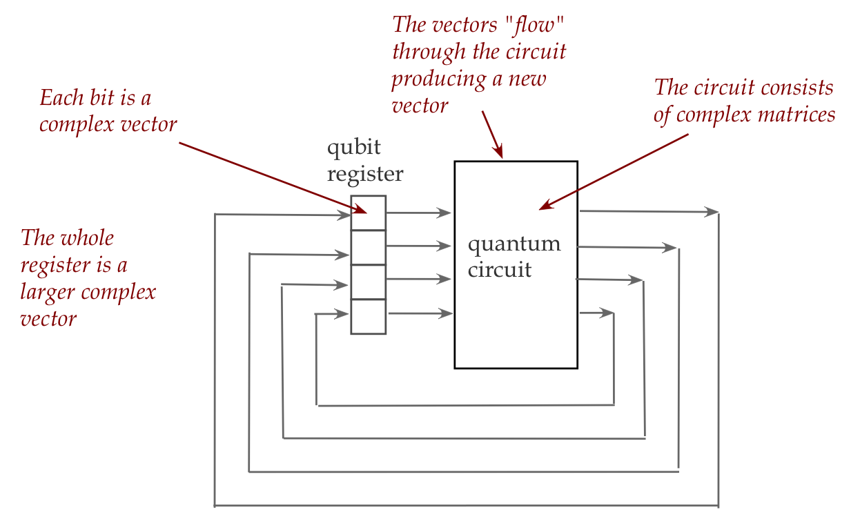
- For the moment we will describe a conceptual view
that is actually implemented in wildly different ways
\(\rhd\)
The actual physical implementation can be quite different
- The starting point is not a binary number but a
(complex) vector:
- We will see that each qubit is actually a small vector.
- A collection of qubits is also a (larger) vector.
- Just as logic gates "act" on regular bits, in a quantum
circuit it is matrices that "act" on vectors.
- There are going to be two fundamentally different kinds
of matrices, and they "act" quite differently.
- One kind is called unitary and acts in the way we're
already familiar with: the matrix multiplies into the input vector.
- The other kind is called Hermitian and the way
it "acts" on a vector is a little strange.
- In a physical realization, of course, there are physical
devices (such as lasers) that achieve the job of these matrices.
Thus, there's no getting around the need to be really comfortable
with the essential linear algebra needed for quantum computing:
the linear algebra of complex vectors with two special types of matrices.
Shall we begin?
2.2
Complex numbers: a review
What are they and where did they come from?
- Consider an equation like \(x^2 = 4\).
\(\rhd\)
We know that \(x=2\) and \(x=-2\) are
solutions (written as \(x = \pm 2\)).
- What about \(x^2 = 2\)?
\(\rhd\)
Doesn't change the concept: \(x = \pm \sqrt{2}\).
- However, \(x^2 = -2\) poses a problem.
\(\rhd\)
No square of a real number is negative
- Suppose we invent the "number" \(\sqrt{-1}\) and give it a
symbol:
$$ i \eql \sqrt{-1} $$
Then using the rules of algebra
$$ (i \sqrt{2})^2 \eql i^2 (\sqrt{2})^2 \eql (\sqrt{-1})^2 (\sqrt{2})^2
\eql (-1) (2) \eql -2 $$
gives a solution to the previous equation.
- In general, a complex number is written
as \(a + ib\) or \(a + bi\)
where \(a\) and \(b\) are real numbers.
- The \(a\) in \(a+ib\) is called the real part.
- \(b\) is called the imaginary part.
- Examples:
| Complex number |
Real part |
Imaginary part |
| \(3 + 4i\) |
\(3\) |
\(4\) |
| \(1.5 + 3.141 \: i\) |
\(1.5\) |
\(3.141\) |
| \(2.718\) |
\(2.718\) |
\(0\) |
| \(8i\) |
\(0\) |
\(8\) |
- Why should this make sense?
- We want to include all real numbers in the set of
complex numbers
\(\rhd\)
This works when \(b=0\) in \(a + ib\)
- However, we need to define arithmetic operations carefully
so that when \(b=0\) the same operations work for real numbers.
- That is,
operations defined on complex numbers should give the expected
results when applied to complex numbers with only real parts
- Luckily, the straightforward algebra works: define
- Addition: \( (a+ib) + (c+id) \defn (a+c) + i(b+d)\)
- Multiplication: \( (a+ib)(c+id) \defn (ac-bd) + i(ad+bc) \)
Notice: we simply treated the real numbers \(a,b,c,d\) and \(i\)
as symbols and used standard algebra (factoring and distribution).
- Recall: the symbol \(\defn\) means "defined as"
- Examples:
$$\eqb{
(4 + 3i) + (3 + 2i) & \eql & 7 + 5i
& & & &\mbx{Add real parts and imag parts separately}\\
(4 + 3i) (3 + 2i) & \eql & (12 - 6) + (8 + 9) i &
& \eql & 6 + 17i
& \mbx{Apply multiplication rule}\\
}$$
- Notice that the multiplication rule satisfies our original
starting point with \(a=0, b=1\):
$$
(0 + i)(0 + i) \eql (0\;0 + 0i + 0i + i^2) \eql i^2 \eql -1
$$
- Multiplication by a real-number scalar:
$$
\beta (a + ib) \eql (\beta a + i(\beta b))
$$
- Subtraction and division:
- Subtraction simply negates the real numbers of the second
complex number, as in:
$$
(a + ib) - (c + id) \eql (a + ib) + ( (-c) + i(-d) )
$$
- Division needs a bit more thought:
$$
\frac{a + ib}{c + id}
\eql
\frac{a + ib}{c + id}
\frac{c - id}{c - id}
\eql
\frac{1}{c^2 + d^2}
(a + ib)(c - id)
$$
Which now becomes a multiplication of two complex numbers, followed
by a scalar multiplication.
Note: we exploited the cancellation in
$$
(c + id) (c - id) \eql c^2 - i^2d^2 + (c)(id) - (c)(id) \eql c^2 + d^2
$$
- Notation:
- We will typically write a complex number symbolically as \(a + ib\)
- But particular values might be written as \(3 + 4i\) because
that's more natural than \(3 + i4\).
- It takes some getting used to, but you should see \(3+4i\) as
one number.
- When reading, your eyes should locate the \(i\) in \(3+4i\)
so that you separately see the imaginary part \(4\).
- About the meaning of a complex number:
- A real number always has physical interpretations, like length.
- A complex number does not directly correspond to anything physical.
- Instead, it's best to think of it as abstraction that leads
to predictive power.
- When we need to predict a physical quantity, we'll be sure to extract
a real number.
- We should also point out a downside to complex numbers:
there's no natural ordering
- We can't say whether \(3+4i\) is less than \(4+3i\) or the other
way around
- Fortunately, this issue is not going to impact our needs.
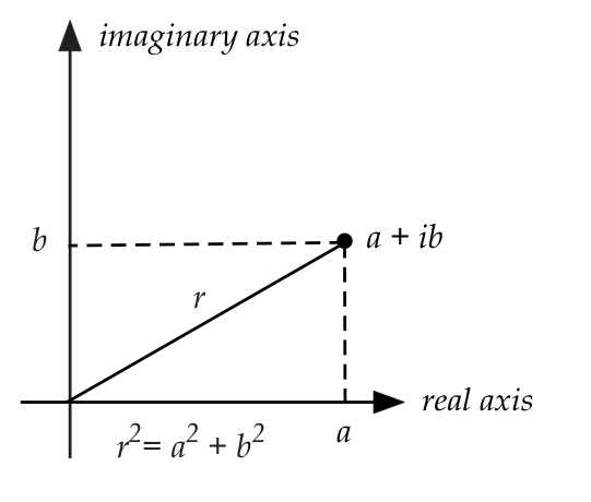
Polar representation of complex numbers:
- One useful graphical representation is obvious when we write
complex number \(z\) as \(z = x + iy\).
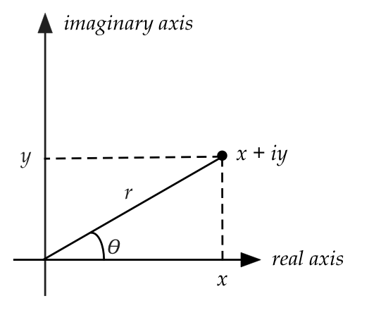
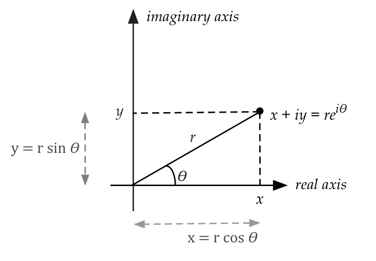
- Given this, one can easily write
$$\eqb{
z & \;\; = \;\; & x + i y \\
& = & r\cos(\theta) + i r \sin(\theta) \\
& = & r \left( \cos(\theta) + i \sin(\theta) \right) \\
}
$$
Once arithmetic has been defined, we can define
functions on complex numbers:
- For example, define for complex number \(z\)
$$
f(z) \eql 2z^2 + 3z + 4 \mbx{Right side has only arithmetic ops}
$$
- An important observation made by Euler:
Suppose you define
$$
e^z \;\; \defn \;\;
1 + z + \frac{z^2}{2!} + \frac{z^3}{3!} + \ldots
$$
analogous to the Taylor series for the real function \(e^x\)
$$
e^x \eql
1 + x + \frac{x^2}{2!} + \frac{x^3}{3!} + \ldots
$$
- Note: the right side has only arithmetic operations.
- Then substituting \(z= i\theta\), and separating
out alternate terms:
$$\eqb{
e^{i\theta} & \;\; = \;\; &
1 + i\theta + \frac{(i\theta)^2}{2!} + \frac{(i\theta)^3}{3!} + \ldots
\\
& \vdots & \mbx{some algebra} \\
& \;\; = \;\; &
\mbox{(series for \(\cos(\theta)\))} +
i \mbox{ (series for \(\sin(\theta)\)) } \\
& \;\; = \;\; &
\cos(\theta) + i \sin(\theta)
}
$$
This (famous and extremely useful) result
$$
e^{i\theta} \eql \cos(\theta) + i \sin(\theta)
$$
is called Euler's relation.
- More generally, \(re^{i\theta} = r(\cos(\theta) + i \sin(\theta))\)
- Think of \(z = re^{i\theta}\) as the polar
representation of the complex number
$$
z \eql x+iy \eql r(cos(\theta) + i \sin(\theta)) \eql re^{i\theta}
$$
- Let's revisit some operations with the polar form
\(z_1 = r_1e^{i\theta_1}\) and \(z_2 = r_2e^{i\theta_2}\)
$$\eqb{
z_1 z_2
&\eql & r_1 r_2 e^{i(\theta_1 + \theta_2)}\\
\frac{z_1}{z_2}
&\eql & \frac{r_1}{r_2} e^{i(\theta_1 - \theta_2)}\\
z_1^{-1} & \eql & \frac{1}{r_1}e^{-i\theta_1} \\
}$$
(Addition requires going back to regular non-polar form.)
- Sometimes an abundance of parentheses can be confusing,
so we often simplify
\(r(\cos(\theta) + i \sin(\theta))\) to
$$
r(\cos\theta + i \sin\theta).
$$
where it's understood that \(\theta\) is the argument to \(\cos\)
and \(\sin\).
- Redundancy in \(\theta\):
- While different values of \(a\) and \(b\) will
result in different complex numbers \(a + ib\), the same is not true
for \(r, \theta\).
- Because, for any integer \(k\)
$$\eqb{
\sin(\theta + 2\pi k) & \eql & \sin\theta \\
\cos(\theta + 2\pi k) & \eql & \cos\theta
}$$
- In polar form
$$\
e^{i(\theta + 2\pi k)} \eql e^{i\theta}
$$
- Thus, for example, \(3e^{i(\frac{\pi}{3} + 6\pi)}\) and
\(3e^{i \frac{\pi}{3}}\) are the same number.
- We will generally prefer to use the smallest angle
when two or more angles are equivalent.
- So, between \(3e^{i(\frac{\pi}{3} + 6\pi)}\) and
\(3e^{i \frac{\pi}{3}}\), we'll use \(3e^{i \frac{\pi}{3}}\).
- This smallest angle is called the principal phase
or principal angle.
- See the solved problems for why this matters.
- Thus, two numbers in polar form
\(r_1e^{i\theta_1}\) and \(r_2e^{i\theta_2}\)
are equal if and only if \(r_1 = r_2\)
and \(\theta_1 = \theta_2 + 2\pi k\) for some integer \(k\).
Conjugates:
- It turns out to be really useful to define something called
a conjugate of a complex number \(z = a+ib\):
$$\eqb{
z^* \;\; & = & \;\; (a + ib)^* \\
\;\; & \defn & \;\; a - ib
}$$
- Then,
$$\eqb{
z z^\ast & \eql & (a + ib)\; (a + ib)^* \\
& \eql & (a + ib)\; (a - ib) \\
& \eql & a^2 + b^2
}$$
Which is a real number.
- The magnitude of a complex number \(z = a+ib\) is
the real number
$$
|z| \;\; \defn \;\; \sqrt{a^2 + b^2} \;\; = \;\; \sqrt{zz^*}
\;\; = \;\; \sqrt{z^* z}
$$
- The magnitude, we have seen, has a geometrical interpretation
to complex numbers: the distance from the origin to
the point representing \(z\).
- Thus, in polar form
$$
\left| re^{i\theta} \right|
\eql
|r| |e^{i\theta}|
\eql
r
$$
because \(|e^{i\theta}|^2 = |\cos\theta + i\sin\theta|^2
= \cos^2\theta + \sin^2\theta = 1\)
- Useful rules to remember about conjugation:
$$\eqb{
(z^*)^* & \eql & z \\
(z_1 + z_2)^* & \eql & z_1^* + z_2^*\\
(z_1 - z_2)^* & \eql & z_1^* - z_2^*\\
(z_1 z_2)^* & \eql & z_1^* z_2^*\\
\left( \frac{z_1}{z_2} \right)^* & \eql & \frac{z_1^*}{z_2^*}
}$$
- And, most importantly, the polar form of
conjugation:
$$\eqb{
(re^{i\theta})^*
& \eql & \left(r \left(\cos\theta + i\sin\theta \right)\right)^* \\
& \eql & r \left(\cos\theta - i\sin\theta \right) \\
& \eql & r \left(\cos\theta + i\sin(-\theta) \right) \\
& \eql & re^{-i\theta}
}$$
Note: we used parens only when needed above.
- Polar conjugation often allows simplification as in:
\(|e^{i\theta}|^2 = (e^{i\theta})^* e^{i\theta} =
e^{-i\theta} e^{i\theta} = 1\)
- We will commonly see the case when \(r=1\) (unit length),
in which case it simplifies to \(e^{-i\theta}\).
- Alternate notation for conjugation:
- Math books often use a "bar" to denote conjugation:
$$\eqb{
\overline{z} \;\; & = & \;\; \overline{a + ib} \\
\;\; & = & \;\; a - ib
}$$
- We will generally prefer the * notation because we'll want
to conjugate entire matrices.
Additional notation:
- Notation for the real and imaginary parts of \(z = a + ib\):
$$\eqb{
\re z \eql a\\
\im z \eql b\\
}$$
- To extract the polar angle, one uses \(\arg\), but
because many angles are equivalent, one gets a set:
$$
\arg z \eql \{\theta: re^{i \theta}=z\}
$$
- When a particular angle is specified, as in
\(2e^{i \frac{\pi}{3}}\),
then the angle (in radians) is often called the phase.
- Notice that multiplication by \(e^{i \phi}\) changes the
phase:
$$
e^{i \phi} \; 2e^{i \frac{\pi}{3}} \eql 2e^{i (\frac{\pi}{3} + \phi)}
$$
This is a notion we will return to frequently in the future.
In-Class Exercise 1:
Review these examples
and then solve:
- Compute \(|z|\) when \(z=4-3i\)
- Express \(3-3i\) in polar form.
- Show that \(\im( 2i(1+4i) - 3i(2-i) ) = -4\)
- Write \(\frac{1}{(1-i)(3+i)}\) in \(a+ib\) form.
- If \(z = i^{\frac{1}{3}}\), what is the phase of \(z^*\) in degrees?
(Hint: there are three cube roots; express \(i\) in polar form to
see why.)
In-Class Exercise 2:
Suppose \(z=z^*\) for a complex number \(z\). What can you
infer about the imaginary part of \(z\)?
2.3
Complex vectors (in old notation)
Because the (forthcoming) Dirac notation takes getting used to, we'll
first look at complex vectors in the notation used in
linear algebra courses.
A vector with complex numbers as elements is a complex vector:
Inner product convention:
- Most math books use a different inner-product definition,
where the right vector is conjugated:
$$
{\bf u} \cdot {\bf v} \eql
u_1 v_1^* + u_2 v_2^* + \ldots +
u_n v_n^*
$$
- However, we will use the convention from physics,
where the left vector is conjugated:
$$
{\bf u} \cdot {\bf v} \eql
u_1^* v_1 + u_2^* v_2 + \ldots +
u_n^* v_n
$$
- Consider the complex numbers \(u_1=(2+3i)\) and
\(v_1=(3+4i)\). Then
$$\eqb{
u_1 v_1^* & \eql & (2+3i) {(3+4i)}^*
& \eql & (2+3i) (3-4i)
& \eql & (18 + i) \\
u_1^* v_1 & \eql & {(2+3i)}^* (3+4i)
& \eql & (2-3i) (3+4i)
& \eql & (18 - i) \\
}$$
- So, the definitions will result in different inner-products
but \({\bf u}\cdot{\bf u} = |{\bf u}|^2\) still holds,
and the real part is the same.
- The convention in physics and quantum computing is to
left-conjugate, and that is what we will do.
- Incidentally, did you notice that in the above
example \( u_1 v_1^* = (u_1^* v_1)^*\)?
2.4
Complex vectors (again) with Dirac notation
Let's first revisit two aspects of real vectors:
- Symbolic convention:
- Most linear algebra textbooks use boldface or arrow notation
for vectors as in:
$$
{\bf u} \eql \vecthree{1}{2+i}{3i}
\;\;\;\;\;\;\;\;
\vec{v} \eql \vecthree{2}{1}{i}
$$
- These are typically subscripted for multiple related vectors,
as in:
$$\eqb{
{\bf w}_1 & \eql & \vecthree{1}{-2}{3}
\;\;\;\;\;\;\;\;
{\bf w}_2 & \eql & \vecthree{2}{0}{1}
}$$
- Dot product:
- The dot product for real vectors is,
not surprisingly, written with a dot:
$$
{\bf w}_1 \cdot {\bf w}_2
\eql
\vecthree{1}{-2}{3} \cdot \vecthree{2}{0}{1}
\eql 5
$$
The result is a number.
- We can treat each real vector as a single-column matrix and instead write
the dot-product as:
$$
{\bf w}_1^T {\bf w}_2
\eql
\mat{1 & -2 & 3} \cdot \vecthree{2}{0}{1}
\eql 5
$$
Here, with a slight abuse of notation, the
\(1\times 1\) result can be interpreted as a number.
- Note: for a complex vector, we'll need to both transpose
and conjugate the left vector:
$$\eqb{
{\bf u} \cdot {\bf v}
& \eql &
({\bf u}^*)^T {\bf v} \\
& \eql &
\left( \mat{1 \\ (2-i) \\ 3i}^* \right)^T \vecthree{2}{1}{i} \\
& \eql &
\left( \mat{1 \\ (2+i) \\ -3i} \right)^T \vecthree{2}{1}{i} \\
& \eql &
\mat{1 & (2+i) & -3i} \vecthree{2}{1}{i} \\
& \eql &
7 + i
}$$
- We could have transposed first and then conjugated:
$$\eqb{
({\bf u}^*)^T {\bf v}
& \eql &
\left( \mat{1 \\ (2-i) \\ 3i}^T \right)^* \vecthree{2}{1}{i} \\
& \eql &
\left( \mat{1 & (2-i) & 3i} \right)^* \vecthree{2}{1}{i} \\
& \eql &
\mat{1 & (2+i) & -3i} \vecthree{2}{1}{i} \\
& \eql &
7 + i
}$$
The first thing to do is to invent notation for
combined tranpose and conjugation: the dagger notation
$$
{\bf u}^\dagger \eql \left[
{u}_1^* \; \ldots \; {u}_n^*
\right]
$$
Then, we can write
$$
({\bf u}^*)^T {\bf v} \eql ({\bf u}^T)^* {\bf v}
\eql {\bf u}^\dagger {\bf v}
$$
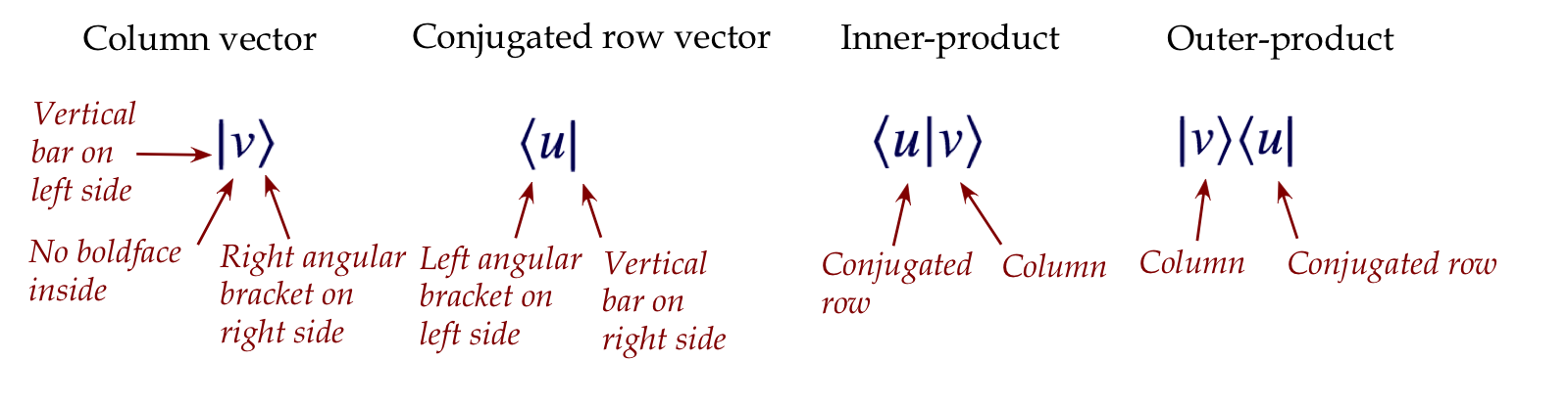
Now on to Dirac notation for vectors:
- A column vector is written as in these examples:
$$
\kt{v} \eql \vecthree{2}{1}{i}
\;\;\;\;\;\;\;\;\;\;\;
\kt{u} \eql \mat{1 \\ (2-i) \\ 3i}
$$
- A conjugated row vector is written as
$$
\br{u} \eql (\kt{u})^\dagger \eql
\mat{1^* & (2-i)^* & (3i)^*}
\eql
\mat{1 & 2+i & -3i}
$$
- And, most crucially, the dot product of
\(\kt{u}\) and \(\kt{v}\) is written as
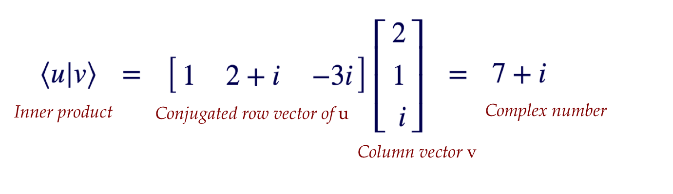
- Symbolically for general vectors
\(\kt{u}=(u_1,\ldots,u_n)\) and
\(\kt{v}=(v_1,\ldots,v_n)\),
$$
\bkt{u}{v}
\eql
\sum_i u_i^* v_i
$$
- This is also commonly called the inner product.
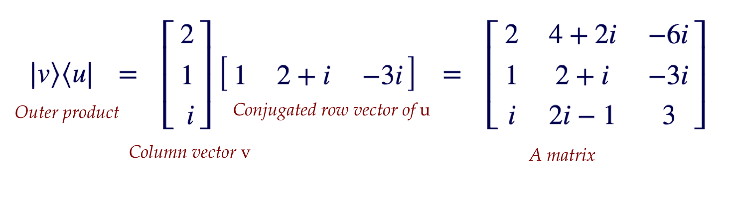
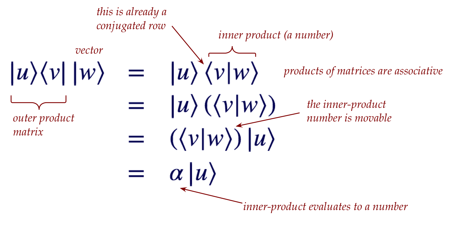
- Next, we'll use the same notation to write an
outer product:
- To summarize:
One needs to be careful with subscripts:
- In traditional notation, we wrote a collection of vectors
\({\bf u}_1, {\bf u}_2, \ldots, {\bf u}_n\) with subscripts not boldfaced.
- In Dirac notation, a collection of \(n\) vectors is
described as: \(\kt{u_1},\kt{u_2},\ldots, \kt{u_n}\)
\(\rhd\)
The subscripts are inside the asymmetric brackets.
- Unfortunately, this can lead to confusion when we
want to describe the individual numbers in a vector, as in:
\(\kt{v} = (v_1,v_2,\ldots,v_n)\)
- Thus, one needs to infer the correct meaning from the context.
Scalars and scalar conjugation:
- First consider an example with real scalars and vectors:
$$
3 \; \vecthree{1}{-2}{3} \eql \vecthree{3}{-6}{9}
$$
Note:
- The result is the same in row form:
$$
3 \; \mat{1 & -2 & 3} \eql \mat{3 & -6 & 9}
$$
- Symbolically, if \({\bf w}=(w_1,w_2,\ldots,w_n)\) is
a real vector and \(\alpha\) is a real number, then:
$$
(\alpha {\bf w})^T \eql \alpha {\bf w}^T
$$
- In our example:
$$
\left( 3 \; \vecthree{1}{-2}{3} \right)^T
\eql
3 \; \mat{1 & -2 & 3}
$$
- But, because we conjugate complex vectors when transposing,
the scalar can get conjugated.
- Let's first look at this symbolically:
- Suppose \(\kt{w}=(w_1,\ldots,w_n)\) is a complex vector and
\(\alpha\) a complex number.
- Then we'll use the notation \(\kt{\alpha w}\)
to mean
$$
\kt{\alpha w}
\eql
\vecthree{\alpha w_1}{\vdots}{\alpha w_n}
\eql \alpha \vecthree{w_1}{\vdots}{w_n}
\eql \alpha \kt{w}
$$
where \(\alpha\) multiplies into each number in the vector.
- In contrast, observe that
$$\eqb{
\br{\alpha w} & \eql &
\mat{(\alpha w_1) & \cdots & (\alpha w_n)}^*\\
& \eql &
\mat{(\alpha w_1)^* & \cdots & (\alpha w_n)^*} \\
& \eql &
\mat{\alpha^* w_1^* & \cdots & \alpha^* w_n^*}\\
& \eql &
\alpha^* \mat{w_1^* & \cdots & w_n^*} \\
& \eql &
\alpha^* \br{w}
}$$
Thus, when a scalar is factored out of a conjugated-row, the
scalar becomes conjugated.
- An example:
- Suppose
$$
\alpha=(2-3i), \;\;\;\;\;\;\;\;
\kt{w} = \vecthree{1}{-2}{3}
$$
- Then, in this case
$$
\br{w} = \mat{1 & -2 & 3}
$$
(The conjugate of a real number is the same real number.)
- Next,
$$
\alpha \kt{w}
\eql
(2-3i) \vecthree{1}{-2}{3}
\eql
\vecthree{2-3i}{-4+6i}{6-9i}
$$
That is, the scalar multiplies each element in the usual way.
- If we conjugate and transpose the result, we get
$$
(\alpha \kt{w})^\dagger
\eql
\left(\vecthree{2-3i}{-4+6i}{6-9i}\right)^\dagger
\eql
\mat{2+3i & -4-6i & 6+9i}
$$
which is NOT equal to \((2-3i)\mat{1 & -2 & 3}\), i.e.,
not equal to \(\alpha \br{w}\)
- But
$$
\mat{2+3i & -4-6i & 6+9i}
\eql
(2+3i) \mat{1 & -2 & 3}
\eql
\alpha^* \br{w}
$$
- That is,
$$
(\alpha \kt{w})^\dagger \eql
\alpha^* \br{w}
$$
- Lastly, for the (squared) magnitude of a vector \(\kt{u}\),
note that
$$
\magsq{\kt{u}} \eql \inr{u}{u}
$$
Why? Recall: that's how we arrived at the definition of inner product!
- When the context makes it clear, we'll simplify the
(not-squared) magnitude notation to \(|u|\).
Vector operations:
- We've already seen scalar multiplication and inner product.
- The only other operation needed is plain old addition, which
is the same as in real vectors, for example:
$$
\vecthree{2}{1}{i} + \vecthree{1}{-2}{3}
\eql \vecthree{3}{-1}{3+i}
$$
- Notationally, we write this in two equivalent ways:
$$
\kt{v + w} \; \defn \; \kt{v} + \kt{w}
$$
Note:
- The right side is easy: it's merely element-by-element
addition of two vectors to give a third.
- The left side is a bit strange because we haven't said
anything about what \(v+w\) means inside the Dirac brackets.
\(\rhd\)
The above definition clarifies.
Scalar "movement":
- There is a type of algebraic simplification we often see
in quantum computing that's worth highlighting.
- We'll do so with real vector examples, but the same idea applies
to complex vectors.
- Consider \(\kt{v}=(3,1)\) and \(\alpha=5\):
- We typically write the scalar multiplication as:
$$
5 \; \vectwo{3}{1}
$$
- We could just as correctly write it as:
$$
\vectwo{3}{1} \; 5
$$
- In this sense, the scalar is "movable" when applied as a multiplier.
- This matters when the scalar itself comes as a result
of an inner product.
- For example, suppose \(\kt{u}=(1,2), \kt{v}=(3,1)\):
- Then, consider the outer-product (matrix) \(\otr{v}{v}\)
times the vector \(\kt{u}\):
$$\eqb{
\left( \otr{v}{v} \right) \; \kt{u}
& \eql &
\left( \vectwo{3}{1} \mat{3 & 1} \right) \; \vectwo{1}{2}\\
& \eql &
\left( \mat{9 & 3\\3 & 1} \right) \; \vectwo{1}{2} \\
& \eql &
\vectwo{15}{5}
}$$
- Instead, observe that we can do this differently by
exploiting matrix-associativity:
$$\eqb{
\left( \otr{v}{v} \right) \; \kt{u}
& \eql &
\kt{v} \left( \inr{v}{u} \right) \\
& \eql &
\vectwo{3}{1} \left( \mat{3 & 1} \vectwo{1}{2} \right) \\
& \eql &
\vectwo{3}{1} \left( 5 \right) \\
& \eql &
5 \; \vectwo{3}{1} \\
& \eql &
\vectwo{15}{5}
}$$
- Symbolically, a movable scalar might represent an
inner-product, which when moved, results in simplification:
$$
\parenl{ \otr{v}{v} } \; \kt{u}
\eql
\kt{v} \parenl{ \inr{v}{u} }
\eql
\parenl{ \inr{v}{u} } \kt{v}
$$
This simplification occurs often enough to be worth memorizing.
Linear combinations:
- Combining scalar multiplication and addition gives us
a linear combination, and some notation for it:
$$
\kt{\alpha u + \beta v} \; \defn \;
\alpha\kt{u} + \beta\kt{v}
$$
- For conjugated rows, we need to conjugate the scalars:
$$
\br{\alpha u + \beta v} \; \defn \;
\alpha^*\br{u} + \beta^*\br{v}
$$
- This leads to two forms of inner products with linear combinations:
$$\eqb{
\inrs{u}{\alpha v + \beta w} & \eql & \alpha\inr{u}{v} + \beta\inr{u}{w}
& \mbx{Linearity on the right}\\
\inrs{\alpha u + \beta v}{w} & \eql & \alpha^*\inr{u}{w} + \beta^*\inr{v}{w}
& \mbx{Conjugate linearity on the left}\\
}$$
Both are important to remember!
- How to read the notation \(\kt{\alpha u + \beta v}\):
- First start with \(u\) and \(v\) as regular column vectors, as in
$$
\kt{u} \eql \vecthree{1}{2-i}{3i}
\;\;\;\;\;\;
\kt{v} \eql \vecthree{2}{1}{i}
$$
- Then compute the column vector \(\alpha u + \beta v\),
for example with \(\alpha=(2-3i), \beta=-1\):
$$
\alpha u + \beta v \eql (2-3i)\vecthree{1}{2-i}{3i}
+ (-1) \vecthree{2}{1}{i}
\eql
\vecthree{-3i}{-8i}{9+5i}
$$
- This is already a column, so we can write it as
$$
\kt{\alpha u + \beta v} \eql \vecthree{-3i}{-8i}{9+5i}
$$
- How to read the notation \(\br{\alpha u + \beta v}\):
- First think of \(\alpha u + \beta v\) as the column
$$
\alpha u + \beta v \eql \vecthree{-3i}{-8i}{9+5i}
$$
- Now conjugate and transpose:
$$
\br{\alpha u + \beta v} \eql \mat{3i & 8i & 9-5i}
$$
- Important:
The above notation for linear combinations is worth re-reading
several times: we will use this frequently throughout the course.
In-Class Exercise 3:
Prove the two results stated above, and one more:
- \(\inrs{u}{\alpha v + \beta w} = \alpha\inr{u}{v} + \beta\inr{u}{w}\)
- \(\inrs{\alpha u + \beta v}{w} = \alpha^*\inr{u}{w} + \beta^*\inr{v}{w}\).
- \(\inr{u}{v} = \inr{v}{u}^*\).
In-Class Exercise 4:
Review these examples
and then solve the following. Given
\(\kt{u}=\mat{\isqt{1}\\ \isqt{i}}, \; \kt{v}=\mat{\isqt{1} \\ \isqt{i}},
\; w=(1,0), \; \alpha=i, \; \beta=-\sqrt{2}i\),
calculate (without converting \(\sqrt{2}\) to decimal format):
- \(\alpha\kt{v}, \kt{\alpha v}, \br{\alpha u}, \; \alpha^*\br{u}\);
- \(\inr{u}{v}\);
- \(\otr{u}{v}\), \(\otr{u}{v}\kt{w}\), and \(\inr{v}{w}\kt{u}\),
and compare the latter two results;
- \(\magsq{\kt{u}}, \inr{u}{u}\);
- \(\inrs{w}{\alpha u + \beta v}\) and
\(\alpha\inr{w}{u} + \beta\inr{w}{v}\);
- \(\inrs{\alpha u + \beta v}{w}\) and
\(\alpha^*\inr{u}{w} + \beta^*\inr{v}{w}\).
Conjugating and transposing a matrix:
- Just as the "dagger" transposes and conjugates a vector,
the same can be applied to a matrix.
- For example:
Let
$$
A \eql \mat{1+i & -i\\
i & 1+i}
$$
Then the transpose is
$$
A^T \eql \mat{1+i & i\\
-i & 1+i}
$$
And the conjugate of the transpose is:
$$
A^\dagger \eql (A^T)^* \eql \mat{1-i & -i\\
i & 1-i}
$$
- The matrix \(A^\dagger\) is called the adjoint of \(A\).
Abbreviated highlights from sections 2.1-3.4
- Complex numbers:
- Either \(z = a + ib\) or \(z = re^{i\theta}\)
- Conjugate: \(z^* = a - ib = re^{-i\theta}\)
- Euler's: \(e^{i\theta} = \cos\theta + i \sin\theta\)
- Rules for arithmetic.
- From which, (complex-valued) functions \(f(z)\)
- Complex vectors:
- Complex numbers as (column) vector elements
$$
\kt{u} \eql \mat{1\\ 2-i\\ 3i}
\;\;\;\;\;\;
\kt{v} = \mat{2 \\ 1\\ i}
$$
- Conjugated row-vector:
$$\eqb{
\br{u} & \eql & \kt{u}^\dagger & \eql & \mat{1 & 2+i & -3i} \\
\br{v} & \eql & \kt{v}^\dagger & \eql & \mat{2 & 1 & -i}
}$$
- Inner-product conjugates left side:
$$
\inr{u}{v} \eql \mat{1 & 2+i & -3i} \mat{2 \\ 1\\ i} \eql 7+i
\;\;\;\; \mbx{A number}
$$
- Squared-magnitude (not length) of a complex vector:
\(\magsq{u} = \inr{u}{u}\)
- Outer-product: column times row
- Scalar rules: \(\kt{\alpha v} = \alpha\kt{v}\) and
\(\br{\alpha v} = \alpha^* \br{v}\)
- Inner products with linear combinations:
$$\eqb{
\inrs{u}{\alpha v + \beta w} & \eql & \alpha\inr{u}{v} + \beta\inr{u}{w}
& \mbx{Linearity on the right}\\
\inrs{\alpha u + \beta v}{w} & \eql & \alpha^*\inr{u}{w} + \beta^*\inr{v}{w}
& \mbx{Conjugate linearity on the left}\\
}$$
2.5
Vector spaces, spans, bases, dimension, orthogonality
We're already familiar with these from prior linear algebra
but let's do a quick review using Dirac notation.
In the definitions below, we assume that the vectors
in any set have the same number of elements:
- It is never the case that we want to put,
for example, \((1,-2,3)\) and \((5,6)\) in the same set.
Definitions:
- Span. Given a collection of vectors
\(\kt{v_1}, \kt{v_2}, \ldots, \kt{v_k}\),
the span of these vectors is the set
of all possible linear combinations of these (with
complex scalars):
$$
\mbox{span}(\kt{v_1}, \kt{v_2}, \ldots, \kt{v_k})
\; \defn \;
\setl{ \alpha_1 \kt{v_1} + \alpha_2 \kt{v_2} + \ldots + \alpha_k\kt{v_k}:
\alpha_i \in \mathbb{C} }
$$
Note: just like \(\mathbb{R}\) is the set of all real numbers,
we use \(\mathbb{C}\) for the set of all complex numbers.
- Vector space.
A vector space \(V\) is a set of vectors such that,
for any subset \(\kt{v_1}, \kt{v_2}, \ldots, \kt{v_k}\)
where \(\kt{v_i} \in V\),
$$
\mbox{span}(\kt{v_1}, \kt{v_2}, \ldots, \kt{v_k})
\; \subseteq \;
V
$$
Think of a vector space as: it contains all the linear combinations
of anything inside it.
- The special vector space \(\mathbb{C}^n\):
$$
\mathbb{C}^n \eql \setl{ \kt{v}=(v_1,\ldots,v_n): v_i
\in\mathbb{C} }
$$
That is, the set of all vectors with \(n\) elements,
where each element is a complex number.
- Thus, for example, \((1, 2+i, 3i) \in \mathbb{C}^3\).
- And \((1,0,1,1,0) \in \mathbb{C}^5\).
- Note: \( \mathbb{C}^3\) is not a subset of \( \mathbb{C}^5\).
- Linear independence.
A collection of vectors \(\kt{v_1}, \kt{v_2}, \ldots, \kt{v_k}\)
is linearly independent if
$$
\alpha_1 \kt{v_1} + \alpha_2 \kt{v_2} + \ldots +
\alpha_k\kt{v_k} \eql 0
$$
implies \(\forall i: \alpha_i = 0\).
- Basis. There are multiple equivalent definitions:
- A basis for a given vector space \(V\),
is a set of vectors \(\kt{v_1}, \kt{v_2}, \ldots, \kt{v_n}\)
from \(V\) such that:
- \(\kt{v_1}, \kt{v_2}, \ldots, \kt{v_n}\) are linearly independent.
- \(V = \mbox{span}(\kt{v_1}, \kt{v_2}, \ldots, \kt{v_n})\)
- A basis for a given vector space \(V\),
is a set of vectors \(\kt{v_1}, \kt{v_2}, \ldots, \kt{v_n}\)
from \(V\) such that any vector \(\kt{u}\in V\)
is uniquely expressible as a linear combination of the \(\kt{v_i}\)'s.
That is, there is only one linear combination
\(\kt{u} = \sum_i \alpha_i \kt{v_i}\).
Note: all bases have the same number of vectors. That is, if one
basis has \(n\) vectors, so does any other basis.
- Dimension.
The dimension of a vector space \(V\) is the number of
vectors in any basis, written as \(\mbox{dim}(V)\).
- As a consequence, if \(\mbox{dim}(V)=n\),
any \(n\) linearly independent vectors from \(V\) forms a basis for \(V\).
- Orthogonal vectors.
Two vectors \(\kt{u}\) and \(\kt{v}\) from a vector space \(V\)
are orthogonal if \(\inr{u}{v} = 0\).
- Note: if \(\inr{u}{v} = 0\), then \(\inr{v}{u} = 0\).
- Orthonormal vectors.
Two vectors \(\kt{u}\) and \(\kt{v}\) from a vector space \(V\)
are orthonormal if \(\inr{u}{v} = 0\) and
\(|u| = |v| = 1\) (that is, each is of unit length).
- Orthonormal basis.
An orthonormal basis \(\kt{v_1}, \kt{v_2}, \ldots, \kt{v_n}\)
for a vector space \(V\) is a basis such that
\(\inr{v_i}{v_j}=0\) and \(\inr{v_i}{v_i}=1\).
Expressing a vector in an orthonormal basis:
- If \(\kt{v_1}, \kt{v_2}, \ldots, \kt{v_n}\) is an
orthonormal basis for \(V\), and \(\kt{u}\in V\) is expressed as
$$
\kt{u} \eql \alpha_1 \kt{v_1} + \ldots + \alpha_n \kt{v_n}
$$
then it's easy to calculate each coefficient \(\alpha_i\) as
$$
\alpha_i \eql \inr{v_i}{u}
$$
- It's worth examining why:
$$\eqb{
\inr{v_i}{u} & \eql &
\inrs{v_i}{\alpha_1 v_1 + \alpha_2 v_2 \ldots + \ldots + \alpha_n v_n}
& \mbx{Expand \(\kt{u}\)}\\
& \eql &
\alpha_1\inr{v_i}{v_1} + \alpha_2 \inr{v_i}{v_2}
+ \ldots + \alpha_n \inr{v_i}{v_n}
& \mbx{Right-linearity of inner-product}\\
& \eql &
\alpha_i\inr{v_i}{v_i}
& \mbx{All others are 0}\\
& \eql &
\alpha_i |v_i|^2 & \\
& \eql &
\alpha_i & \mbx{All \(\kt{v_i}\)'s are unit length}\\
}$$
Note: all but one of the inner products are zero.
- The above result can be summarized as:
If \(\kt{u}\) is expressed in terms of orthonormal
basis \(\kt{v_1}, \kt{v_2}, \ldots, \kt{v_n}\)
$$
\kt{u} \eql \alpha_1 \kt{v_1} + \ldots + \alpha_n \kt{v_n}
$$
then the i-th coefficient is merely the inner product
$$
\alpha_i \eql \inr{v_i}{u}
$$
(Remember this!)
- This simplification is a result of both orthogonality
and unit lengths (the "normal" part in orthonormal).
- Some terminology:
- Writing a vector as a linear combination of basis
vectors
$$
\kt{u} \eql \alpha_1 \kt{v_1} + \ldots + \alpha_n \kt{v_n}
$$
is called expanding a vector in a basis.
- The complex scalars \(\alpha_i\) are called
coefficients or amplitudes.
What's important to know about vectors and bases in quantum computing:
- Nearly all vectors encountered will be unit vectors (magnitude = 1).
- When an exception occurs, we typically normalize the
vector to make it unit-length:
$$
\kt{v} \eql \frac{1}{|u|} \kt{u}
$$
- Nearly all bases will be orthonormal bases.
- These properties simplify expressions and calculations
but at first can be a bit confusing.
In-Class Exercise 5:
Suppose \(\kt{u}=(1,0,0,0), \kt{v}=(0,0,1,0)\)
and \(W=\mbox{span}(\kt{u},\kt{v})\).
- Show that \(\kt{u}, \kt{v}\) are linearly independent.
- What is the dimension of \(W\)?
- Express \(\kt{x}=(-i,0,i+1,0)\) in terms of \(\kt{u},\kt{v})\).
- Is \(\kt{u},\kt{v})\) a basis for \(W\)? Explain.
- Is \(W = \mathbb{C}^k\) for any value of \(k\)?
The standard basis for \(\mathbb{C}^n\):
- Define the \(n\) vectors \(\kt{e_1},\ldots,\kt{e_n}\)
where \(\kt{e_i}=(0,0,\ldots,1,\ldots,0)\)
\(\rhd\)
All \(0\)'s with a \(1\) as the i-th element.
- Example: for \(\mathbb{C}^3\):
$$
\kt{e_1} \eql \vecthree{1}{0}{0}
\;\;\;\;\;\;
\kt{e_2} \eql \vecthree{0}{1}{0}
\;\;\;\;\;\;
\kt{e_3} \eql \vecthree{0}{0}{1}
$$
- This basis is often called the standard basis
and sometimes the computational basis.
- Note: the standard basis itself has no complex numbers.
\(\rhd\)
Any complex vector is nonetheless expressible via complex coefficients.
- Example:
$$
\vecthree{1}{2-i}{3i}
\eql
1 \; \vecthree{1}{0}{0}
\;\; + \;\;
(2-i) \; \vecthree{0}{1}{0}
\;\; + \;\;
(3i) \; \vecthree{0}{0}{1}
$$
- We'll shortly see a somewhat unusual but commonly used
notation for the standard basis.
2.6
More about Dirac notation
At this point you may be wondering why we bother with this
"asymmetric" notation?
There are four reasons. The first two are:
- The notation nicely tracks conjugation and transpose.
- For example, consider an outer-product matrix \(\otr{u}{v}\)
times a vector \(\kt{w}\):
- The asymmetric brackets make the conjugation status obvious.
-
Because the brackets delineate a single vector, one can write
something more elaborate in between as in:
- \(\kt{\mbox{3rd qubit}}\)
- \(\br{A u}\), where the operator \(A\) is applied to the
vector \(u\) and then the result is turned into a conjugated row.
We'll now get to the third reason, which is that a convention
has been developed with the notation that greatly eases descriptions
for quantum computing:
The fourth reason is valuable in quantum mechanics:
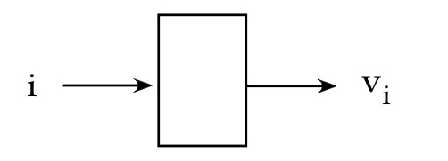
- It turns out that finite-sized vectors generalize to
infinite-sized vectors quite easily:
- A regular vector like \(\kt{v}=(v_1,v_2,\ldots,v_n)\)
has its elements indexed by the integers \(1,2,\ldots,n\).
- Then, when looking at \(v_i\), the \(i\) is an integer
between 1 and n.
- Think of the index i as input, and the element \(v_i\) as output:
- One could define vectors \(\kt{v}=(v_1,v_2,\ldots)\)
where the index set is all the natural numbers: \(1,2,3,\ldots\)
- And one can define vectors with a real-valued index,
where the elements are \(v_x\).
\(\rhd\)
This is really nothing other than the function \(v(x)\).
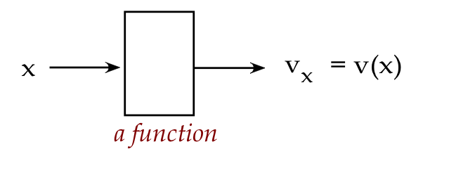
- The Dirac notation is the same for functions:
\(\kt{f(x)}\)
- This fits in with the other kind of generalization that's
needed when going from "finite and discrete" to "infinite and continuous":
\(\rhd\)
An operator is the equivalent generalization of a matrix.
- Again, Dirac notation treats both the same way, allowing
for compact multi-use notation.
Without knowing much more than we've just seen, we can already
work with this notation:
- For example, consider the two vectors
$$
\kt{0} \eql \vectwo{1}{0}
\;\;\;\;\;\;\;\;
\kt{1} \eql \vectwo{0}{1}
$$
- We can easily compute inner products:
$$\eqb{
\inr{0}{0} & \eql & \mat{1 & 0} \vectwo{1}{0} \eql 1 \\
\inr{0}{1} & \eql & \mat{1 & 0} \vectwo{0}{1} \eql 0 \\
\inr{1}{0} & \eql & \mat{0 & 1} \vectwo{1}{0} \eql 0 \\
\inr{1}{1} & \eql & \mat{0 & 1} \vectwo{0}{1} \eql 1 \\
}$$
- And outer products:
$$\eqb{
\otr{0}{0} & \eql & \vectwo{1}{0} \mat{1 & 0} \eql
\mat{1 & 0\\ 0 & 0}\\
\otr{0}{1} & \eql & \vectwo{1}{0} \mat{0 & 1} \eql
\mat{0 & 1\\ 0 & 0}\\
\otr{1}{0} & \eql & \vectwo{0}{1} \mat{1 & 0} \eql
\mat{0 & 0\\ 1 & 0}\\
\otr{1}{1} & \eql & \vectwo{0}{1} \mat{0 & 1} \eql
\mat{0 & 0\\ 0 & 1}\\
}$$
In-Class Exercise 6:
For the vectors \(\kt{00}, \kt{01}, \kt{10}, \kt{11}\)
defined above, compute the outer products
- \(\otr{00}{00}\)
- \(\otr{01}{01}\)
- \(\otr{10}{10}\)
- \(\otr{11}{11}\)
In-Class Exercise 7:
Using the vectors \(\kt{0}, \kt{1}\), compute the vectors
- \(\kt{h_1} = \isqt{1} (\kt{0} + \kt{1})\)
- \(\kt{h_2} = \isqt{1} (\kt{0} - \kt{1})\)
- Show that \(\kt{h_1}, \kt{h_2}\) are orthonormal
(unit length and orthogonal).
- Show that \(\kt{h_1}, \kt{h_2}\) are a basis for
\(\mathbb{C}^2\).
[Hint: start by expressing \(\kt{0}, \kt{1}\)
in terms of \(\kt{h_1}, \kt{h_2}\).]
2.7
Projections and projectors
Because we don't have a convenient way to visualize a 2D
complex vector, let's start with a description
that uses real vectors:
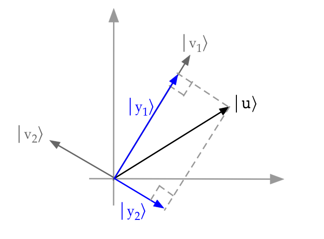
- Here, \(\kt{v_1}, \kt{v_2}\) are orthonormal basis vectors,
and \(\kt{u}\) is a vector.
- The picture shows the projection of \(\kt{u}\) onto
each of \(\kt{v_1}\) and \(\kt{v_2}\).
- Note: when \(\kt{u}\) is unit-length, the projections are
likely to be smaller in length.
- Geometrically with real vectors, a projection is the
shadow cast by one vector on another (with perpendicular light).
- For real vectors, we know (from earlier linear algebra) that:
$$
\kt{y_1}
\eql
\left(
\frac{ \inr{v_1}{u} }{\inr{v_1}{v_1} }
\right) \kt{v_1}
$$
- When \(\kt{v_1}, \kt{v_2}\) are unit-length,
\(\inr{v_i}{v_i} = |v_i|^2 = 1\). Thus
$$
\kt{y_1}
\eql
\inr{v_1}{u} \; \kt{v_1}
$$
Similarly
$$
\kt{y_2}
\eql
\inr{v_2}{u} \; \kt{v_2}
$$
- Most importantly, the two projections geometrically add up
to the original vector:
$$\eqb{
\kt{u} & \eql & \kt{y_1} + \kt{y_2}\\
& \eql &
\inr{v_1}{u} \; \kt{v_1} \; + \; \inr{v_2}{u} \; \kt{v_2}
}$$
What does a projection mean for complex vectors?
- Instead of thinking geometrically, we'll instead focus on
this question:
What (stretched) parts of \(\kt{v_1}, \kt{v_2}\) add up to \(\kt{u}\)?
- So, let's imagine (complex) numbers \(\alpha_1, \alpha_2\)
where
$$
\alpha_1 \kt{v_1} + \alpha_2 \kt{v_2} \eql \kt{u}
$$
- We need to solve for the \(\alpha\)'s. Take
the inner product with \(\kt{v_1}\) on both sides:
$$\eqb{
& &
\inrs{v_1}{\alpha_1 v_1 + \alpha_2 v_2}
& \eql & \inr{v_1}{u}
& \mbx{Use right-side linearity}\\
& \implies &
\alpha_1\inr{v_1}{v_1} + \alpha_2 \inr{v_1}{v_2}
& \eql & \inr{v_1}{u}
& \mbx{\(\inr{v_1}{v_1}=1, \inr{v_1}{v_2}=0\)}\\
& \implies &
\alpha_1
& \eql & \inr{v_1}{u} & \\
}$$
(Recall: the \(v_i\)'s are orthonormal.)
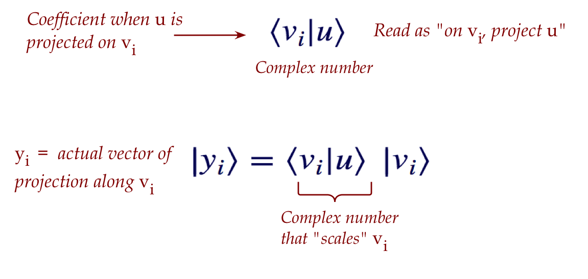
- Thus, the coefficient-of-projection \(\alpha_i\)
is simply the inner product \(\inr{v_i}{u}\).
- In general, we'll have an orthonormal basis
\(\kt{v_1}, \kt{v_2}, \ldots, \kt{v_n}\), where for
each for any vector \(\kt{u}\):
- Example:
- Suppose \(\kt{u}=(\frac{\sqrt{3}}{2}, \frac{1}{2})\)
and \(\kt{v_1}=(\frac{1}{2}, \frac{\sqrt{3}}{2})\)
- Then,
$$\eqb{
\kt{y_1}
& \eql &
\inr{v_1}{u} \; \kt{v_1} \\
& \eql &
\left(
\mat{ \frac{1}{2} & \frac{\sqrt{3}}{2} }
\vectwo{ \frac{\sqrt{3}}{2} }{ \frac{1}{2} }
\right)
\vectwo{ \frac{1}{2} }{ \frac{\sqrt{3}}{2} }
& \eql &
\frac{\sqrt{3}}{2} \;
\vectwo{ \frac{1}{2} }{ \frac{\sqrt{3}}{2} }
& \eql &
\vectwo{ \frac{\sqrt{3}}{4} }{ \frac{3}{4} }
}$$
- Notice that
$$
\magsq{y_1} \eql
\left( \frac{\sqrt{3}}{4} \right)^2
+
\left( \frac{3}{4} \right)^2
\eql \frac{12}{16}
$$
Which is less than unit-length.
- What we will see later: when projections result in
less-than-unit-length vectors, we will normalize (rescale)
them to unit-length.
Projectors or projection matrices:
- Now \(\kt{y_1}\) is the vector that results
from projecting the vector \(\kt{u}\) on \(\kt{v_1}\).
- We know that a matrix multiplying into a vector
transforms it into another vector.
- Thus, one can ask: is there a matrix \(P_1\)
that would achieve this transformation, i.e.
$$
\kt{y_1} \eql P_1 \kt{u}?
$$
- Such a matrix is called a projector matrix.
- Observe that
$$\eqb{
\kt{y_1}
& \eql &
(\inr{v_1}{u}) \; \kt{v_1}
& \mbx{From earlier}\\
& \eql &
\kt{v_1} \; (\inr{v_1}{u})
& \mbx{The scalar in parens can be moved}\\
& \eql &
\left(\otr{v_1}{v_1} \right) \; \kt{u}
& \mbx{Associativity of matrix multiplication}\\
}$$
- But we've seen that the outerproduct \(\otr{v_1}{v_1}\)
is in fact a matrix. So, let's define
$$
P_1 \defn
\otr{v_1}{v_1}
$$
- We have now found our matrix: \(P_1\)
$$
P_1 \kt{u} \eql \otr{v_1}{v_1} \; \kt{u} \eql \kt{y_1}
$$
- Note: \(P_1\) depends only on the basis vector
\(\kt{v_1}\); it does not depend on \(\kt{u}\).
- Just like we dropped boldface notation for vectors, we will
do the same with matrices.
- Generally, we will use unbolded capital letters for matrices,
(the convention in quantum computing/mechanics).
- It does take some getting used to.
- In our example:
$$
\otr{v_1}{v_1}
\eql
\vectwo{ \frac{1}{2} }{ \frac{\sqrt{3}}{2} }
\mat{ \frac{1}{2} & \frac{\sqrt{3}}{2} }
\eql
\mat{
\frac{1}{4} & \frac{\sqrt{3}}{4} \\
\frac{\sqrt{3}}{4} & \frac{3}{4}
}
\; \defn \; P_1
$$
- Then,
$$
P_1 \kt{u}
\eql
\mat{
\frac{1}{4} & \frac{\sqrt{3}}{4} \\
\frac{\sqrt{3}}{4} & \frac{3}{4}
}
\vectwo{ \frac{\sqrt{3}}{2} }{ \frac{1}{2} }
\eql
\vectwo{ \frac{\sqrt{3}}{4} }{ \frac{3}{4} }
\eql
\kt{y_1}
$$
- For our two-vector basis, the other projector is:
$$
P_2 \eql
\otr{v_2}{v_2}
\eql
\vectwo{ \frac{-\sqrt{3}}{2} }{ \frac{1}{2} }
\mat{ - \frac{\sqrt{3}}{2} & \frac{1}{2} }
\eql
\mat{ \frac{3}{4} & -\frac{\sqrt{3}}{4}\\
-\frac{\sqrt{3}}{4} & \frac{1}{4} }
$$
The completeness relation for projectors:
- We'll explain the idea with a two-vector orthonormal basis
\(\kt{v_1}, \kt{v_2}\).
- First, we'll write \(\kt{u}\) as the addition of
\(\kt{u}\)'s projections on \(\kt{v_1}, \kt{v_2}\):
$$\eqb{
I \: \kt{u}
& \eql &
\kt{u} & \mbx{Identity}\\
& \eql &
P_1 \kt{u} + P_2 \kt{u}
& \mbx{A vector is a sum of its projections}\\
& \eql &
\left( P_1 + P_2 \right) \: \kt{u} & \\
}$$
Thus
$$
(P_1 + P_2 - I) \kt{u} \eql {\bf 0}
$$
for all \(\kt{u}\).
- And so, the sum of projectors is the identity matrix:
$$
P_1 + P_2 \eql I
$$
- Let's see this at work with the projectors written as
outerproducts for an \(n\)-vector orthonormal basis:
$$\eqb{
\kt{u}
& \eql &
\parenl{ \inr{v_1}{u} } \: \kt{v_1}
+ \ldots +
\parenl{ \inr{v_n}{u} } \: \kt{v_n}
& \mbx{Each vector with each coefficient}\\
& \eql &
\kt{v_1} \: \parenl{ \inr{v_1}{u} }
+ \ldots +
\kt{v_n} \: \parenl{ \inr{v_n}{u} }
& \mbx{Scalar movement}\\
& \eql &
\parenl{ \otr{v_1}{v_1} } \: \kt{u}
+ \ldots +
\parenl{ \otr{v_n}{v_n} } \: \kt{u}
& \mbx{Associativity}\\
& \eql &
\parenl{ \otr{v_1}{v_1} + \ldots + \otr{v_n}{v_n} }
\: \kt{u}
& \mbx{Factoring}\\
}$$
- That is,
$$
\otr{v_1}{v_1} + \ldots + \otr{v_n}{v_n} \eql I
$$
Or
$$
P_1 + \ldots + P_n \eql I
$$
- Let's work out the completeness relation for the
\(\kt{h_1}, \kt{h_2}\) vectors seen earlier:
- Recall: \(\kt{h_1} = \isqt{1} (\kt{0} + \kt{1})\) and
\(\kt{h_2} = \isqt{1} (\kt{0} - \kt{1})\)
- Then,
$$\eqb{
\otr{h_1}{h_1} + \otr{h_2}{h_2}
& \eql &
\vectwo{\isqt{1}}{\isqt{1}} \mat{\isqt{1} & \isqt{1}}
+
\vectwo{\isqt{1}}{-\isqt{1}} \mat{\isqt{1} & -\isqt{1}} \\
& \eql &
\mat{ \frac{1}{2} & \frac{1}{2}\\
\frac{1}{2} & \frac{1}{2} }
+
\mat{ \frac{1}{2} & -\frac{1}{2}\\
-\frac{1}{2} & \frac{1}{2} } \\
& \eql &
I
}$$
- Notation: Sometimes, for a vector \(\kt{v}\) we'll
use the notation \(P_v\) to denote the projector
\(P_v = \otr{v}{v}\)
In-Class Exercise 8:
For any projector \(\otr{v}{v}\) show that
\( \left( \otr{v}{v} \right)^\dagger = \otr{v}{v}\).
[Hint: you can transpose and then conjugate.]
Note: a matrix \(A\) like \(P_v = \otr{v}{v}\) that
satisfies \(A^\dagger = A\) is called Hermitian, as
we'll see below.
The above result is worth codifying as a formal result:
- Proposition 2.1:
A projector \(P_v = \otr{v}{v}\) equals its own adjoint:
\(P_v^\dagger = P_v\). That is,
\( \left( \otr{v}{v} \right)^\dagger = \otr{v}{v}\).
In-Class Exercise 9:
Using the vectors \(\kt{0}, \kt{1}\), compute the vectors
- \(\kt{y_1} = \isqt{1}\kt{0} + \isqt{i} \kt{1}\)
- \(\kt{y_2} = \isqt{1} \kt{0} - \isqt{i} \kt{1})\)
- Show that \(\kt{y_1}, \kt{y_2}\) are a basis for
\(\mathbb{C}^2\).
- Show the completeness relation for this basis.
Abbreviated highlights from sections 2.5-2.7
- Vector orthogonality (defined as): \(\inr{u}{v} = 0\)
- Orthonormal:
- \(\inr{u}{v} = 0\)
- And \(\mag{u} = \mag{v} = 1\)
- A few important special 2D vectors:
$$\eqb{
\kt{0} & \eql & \mat{1\\ 0} & \;\;\;\;\;\; & \kt{1} & \eql & \mat{0\\ 1}\\
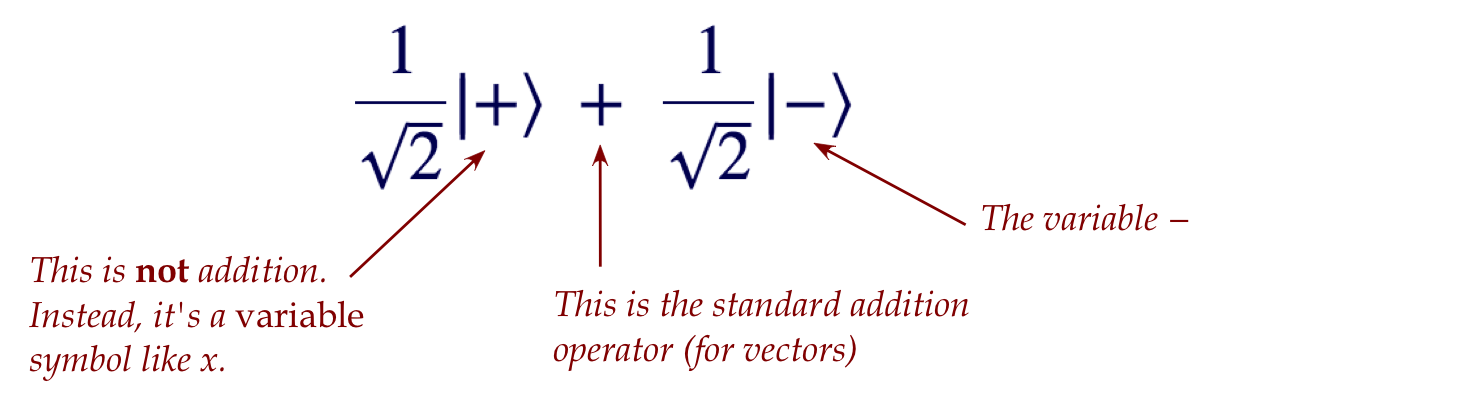
\kt{+} & \eql & \mat{\isqt{1}\\ \isqt{1}} & \;\;\;\;\;\; &
\kt{-} & \eql & \mat{\isqt{1}\\ -\isqt{1}}
}$$
- Projections and projectors:
- Let \(\kt{v_1},\kt{v_2},\ldots\) be an orthonormal basis.
- The projector for \(\kt{v_1}\) (a matrix) is:
$$
P_{v_1} \eql \otr{v_1}{v_1}
$$
- The projection of any \(\kt{u}\) on \(\kt{v_1}\):
$$\eqb{
P_{v_1} \kt{u}
& \eql & \otr{v_1}{v_1} \kt{u} & \mbx{Apply projector} \\
& \eql & \kt{v_1} \; \inr{v_1}{u} & \mbx{Associativity} \\
& \eql & \inr{v_1}{u} \; \kt{v_1} & \mbx{Scalar movement} \\
}$$
The number \(\inr{v_1}{u}\) is the coefficient of projection.
- A vector is the sum of its projections:
$$
\kt{u}
\eql
\parenl{ \inr{v_1}{u} } \: \kt{v_1}
+ \ldots +
\parenl{ \inr{v_n}{u} } \: \kt{v_n}
$$
- Projectors of a basis add up to the identity (completeness relation):
$$
\otr{v_1}{v_1} + \ldots + \otr{v_n}{v_n} \eql I
$$
- Basis orthonormality is key to the simplified expressions above.
Finally, let's summarize projectors through a few pictures (using real vectors):
- First, for any vector \(\kt{v}\), the projector \(\otr{v}{v}\)'s
effect on a vector \(\kt{u}\):
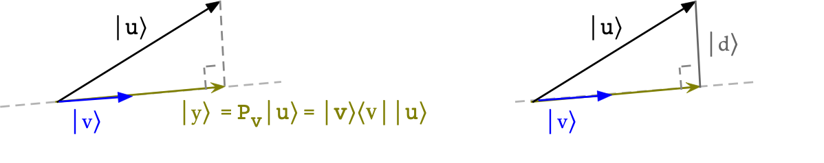
- Think of the projector as some matrix acting on \(\kt{u}\)
to produce some vector \(\kt{y}\):
$$
\otr{v}{v} \; \kt{u} \eql \kt{y}
$$
(Left side of picture)
- Then,
$$
\kt{y} \eql \otr{v}{v} \; \kt{u} \eql \kt{v} \; \inr{v}{u}
\eql \inr{v}{u} \; \kt{v}
$$
- Let's see why \(\otr{v}{v}\) results in the projection:
(Right side of picture)
- If it's a projection, the difference vector \(\kt{d}\)
should be orthogonal to \(\kt{v}\)
- Let's work out the inner product:
$$
\inr{v}{d} \eql
\inrh{v}{ \kt{u} \; - \; \inr{v}{u} \kt{v} }
\eql
\inr{v}{u} \; - \; \inr{v}{u} \; \inr{v}{v}
\eql 0
$$
Which makes it orthogonal.
- Lastly, let's intuit why the projections computed
from an orthonormal basis add up to the original vector \(\kt{u}\):
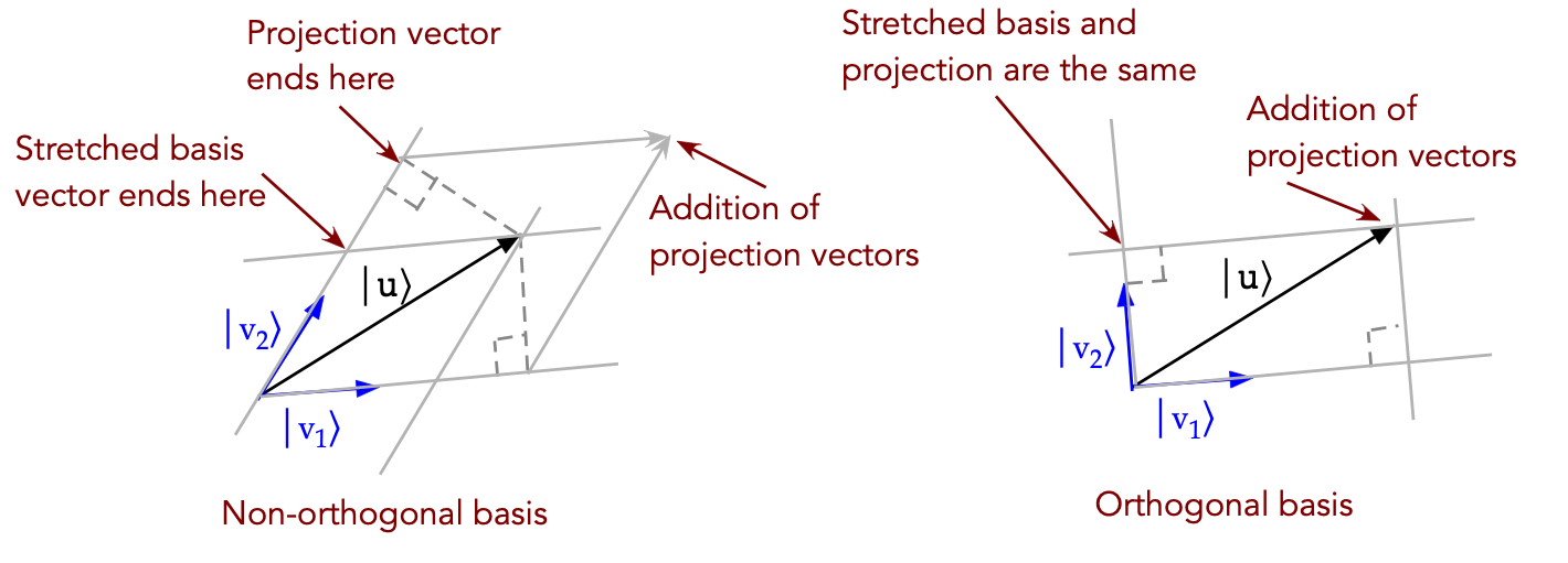
- On the left, we see that projections do not add up to \(\kt{u}\)
if the basis is not orthonormal (parallelogram case)
- On the right, because the parallelogram is a rectangle,
the projections do add up.
2.8
Two important types of operators (matrices): Hermitian and unitary
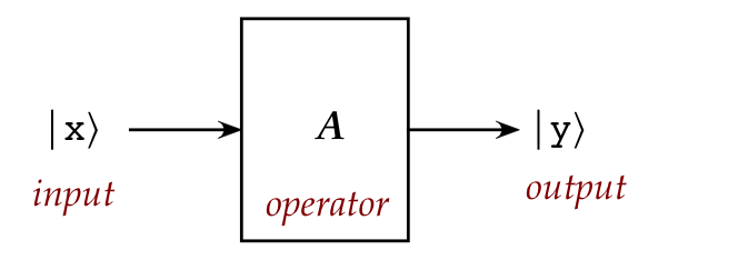
Recall the meaning of the term operator:
The adjoint of a matrix operator:
- Recall: for any matrix \(A\), its adjoint is
the matrix \(A^\dagger\).
- That is: \(A^\dagger\) is the transpose and conjugate
of \(A\).
- Example:
Let
$$
A \eql \mat{1+i & -i\\
i & 1+1}
$$
Then the transpose is
$$
A^T \eql \mat{1+i & i\\
-i & 1+i}
$$
And the conjugate of the transpose is:
$$
A^\dagger \eql (A^T)^* \eql \mat{1-i & -i\\
i & 1-i}
$$
In-Class Exercise 10:
Consider these matrices. (Yes, the latter two have special names.)
$$
A \eql \mat{1 & -i\\
i & 1}
\;\;\;\;\;\;
B \eql \mat{i & 1\\
1 & -i}
\;\;\;\;\;\;
Y \eql \mat{0 & -i\\
i & 0}
\;\;\;\;\;\;
H \eql \mat{\isqt{1} & \isqt{1}\\
\isqt{1} & -\isqt{1}}
$$
Compute
- The adjoints \(A^\dagger, B^\dagger, Y^\dagger, H^\dagger\)
- \(A^\dagger A\), \(Y^\dagger Y\) and \(H^\dagger H\)
- \(A A^\dagger\), \(Y Y^\dagger\) and \(H H^\dagger\)
In computing the adjoint, do we get the same result if
we first apply conjugation and then transpose?
The two kinds of operators we're going to need
are: Hermitian and unitary.
Let's start with Hermitian:
- A Hermitian operator is an operator that
satisfies \(A = A^\dagger\)
- Thus for example
$$
A \eql \mat{1 & -i\\
i & 1}
$$
is Hermitian.
- While
$$
B \eql \mat{i & 1\\
1 & -i}
$$
is not.
- Think of Hermitian as the complex generalization
of a symmetric matrix for real numbers.
\(\rhd\)
A real matrix that's symmetric is Hermitian.
A unitary operator:
- A unitary operator \(A\) is one that satisfies
\(A^\dagger A = A A^\dagger = I\)
\(\rhd\)
That is, \(A^{-1} = A^\dagger\)
- Examples:
- We saw that with
$$
H \eql \mat{\isqt{1} & \isqt{1}\\
\isqt{1} & -\isqt{1}}
$$
\(H^\dagger H = H H^\dagger = I\)
and so \(H\) is unitary.
- But
$$
A \eql \mat{1 & -i\\
i & 1}
$$
is not.
We're going to include a third type of operator that's
closely related to Hermitian operators: projection
- Recall that we used vectors to compute a projection matrix.
- In this spirit of "operator" terminology, we'll call this
a projection operator or projector (as it's sometimes called).
- Recall that when \(\kt{u}\) is projected on \(\kt{v}\), the
resulting vector (along \(\kt{v}\)) is:
$$
\otr{v}{v} \; \kt{u}
$$
- We wrote the outerproduct \(\otr{v}{v}\)
earlier as the projector matrix
$$
P \eql \otr{v}{v}
$$
This is what we mean by the projector or projection operator.
So far all we have are definitions of these three types of
matrices, all of which play a crucial role in anything
quantum-related.
As a preview:
- We'll use unitary matrices to modify qubits.
\(\rhd\)
This will occur by the usual "matrix changes a vector by multiplication"
- Hermitian matrices are quite different:
- They will be used for something called measurement,
a feature unique to quantum systems.
- And we won't be multiplying a vector by a Hermitian matrix
\(\rhd\)
Instead, the matrix will be "applied" to a vector in a rather unusual way
- Projector matrices play a role in the unusual
application of Hermitian matrices, which is why the two
kinds are intimately connected.
Before we get to using these matrices, we'll need to understand
some useful general properties.
As a first step, let's point out something common to all three:
- All three matrices are square.
- Clearly, this is true for any projector:
- A projector is constructed from an outerproduct
of an \(n\times 1\) vector \(\kt{v}\) and a
\(1\times n\) vector \(\br{v}\):
$$
\left( \otr{v}{v} \right)_{n\times n}
$$
- Example:
$$
\vecthree{3}{1}{0} \mat{3 & 1 & 0} \eql
\mat{9 & 3 & 0\\
3 & 1 & 0\\
0 & 0 & 0}
$$
- For a Hermitian operator, the squareness arises from
requiring \(A = A^\dagger\):
- Suppose \(A_{m\times n}\) has m rows, n columns.
- Because \(A^\dagger\) is the conjugate transpose,
\(A^\dagger\) has n rows, m columns.
- The only way we can have \(A = A^\dagger\) is if \(m=n\).
- For unitary operator, the squareness comes from
\(A^{-1} = A^\dagger\):
- We can of course compute \(A^\dagger\) for a non-square
matrix.
- But for this to equal the inverse, we must have
\(A A^\dagger = A^\dagger A = I\).
- Thus, for multiply compatibility on both sides,
\(A\) must be square.
- Because these are the key operators that motivate
the theory, the term operator itself is defined to
be "square".
- This makes sense for matrix operators.
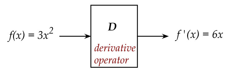
- What about something like the differential operator?
- For more general operators, the generalization of "square"
is the following:
- Consider a vector space \(V\), a set of vectors closed under
linear combinations
\(\rhd\)
Any linear combination of vectors in \(V\) will be in \(V\).
- An operator is something that acts on a vector \(v\in V\)
to produce a vector in \(V\).
- Sometimes this is expressed as: an operator is a mapping
from a vector space to itself.
2.9
Useful properties: adjoints and inner products
Note:
- For the most part, we will use "matrix
proofs" because they are less abstract and amenable to examples.
- More abstract and generalized "slick" proofs do exist,
which we'll use only occasionally.
- Where it makes sense, we'll accompany a proof with an
example to illustrate the main ideas.
- More matrix notation:
- Sometimes we'll use \(a_{ij}\) or \(a_{i,j}\) to denote
the element in row i and column j of a matrix \(A\).
- The above introduces a new symbol, so one often uses
\( (A)_{ij} \) or \( (A)_{i,j} \) directly.
- This has the advantage of conveniently describing the
i-j-th element of a sum as in \( (A+B)_{ij} \).
Let's start with a really useful property when adjoints
occur in an inner-product:
Next, some basic properties of adjoints:
In-Class Exercise 11:
Use
$$
A \eql \mat{1 & -i\\
i & 1}
\;\;\;\;\;\;
B \eql \mat{i & 1\\
1 & -i}
\;\;\;\;\;\;
\alpha = 1+i
$$
as examples in confirming (i)-(iv) above.
2.10
Useful properties: Hermitian operators
Recall the definition of a Hermitian operator:
An operator \(A\) is Hermitian if \(A^\dagger = A\).
Now let's run through some properties:
- Proposition 2.4:
Let \(A, B\) be Hermitian operators. Then
- \(A + B\) is Hermitian
- \(\alpha A\) is Hermitian for real numbers \(\alpha\).
Proof:
For the first part
$$\eqb{
(A + B)^\dagger_{ij}
& \eql & (A + B)^*_{ji}
& \mbx{Conjugate, then transpose} \\
& \eql & (A^* + B^*)_{ji}
& \mbx{Conjugate distributes} \\
& \eql & A^*_{ji} + B^*_{ji}
& \mbx{Matrix addition} \\
& \eql & A^\dagger_{ij} + B^\dagger_{ij}
& \mbx{Definition of conjugate-transpose} \\
& \eql & A_{ij} + B_{ij}
& \mbx{A, B are Hermitian} \\
& \eql & (A+B)_{ij} &
}$$
For the second
$$
(\alpha A)^\dagger_{ij}
\eql (\alpha A)^*_{ji}
\eql (\alpha^* A^*)_{ji}
\eql \alpha A^*_{ji}
\eql \alpha A^\dagger_{ji}
\eql \alpha A_{ij}
\eql (\alpha A)_{ij}
$$
- Example: suppose
$$
Y \eql \mat{0 & -i\\ i & 0}
$$
Then
$$
3Y \eql \mat{0 & -3i\\ 3i & 0}
$$
and
$$
(3Y)^\dagger \eql \mat{0 & -3i\\ 3i & 0}^\dagger
\eql \mat{0 & -3i\\ 3i & 0} \eql 3Y
$$
Which makes \(3Y\) Hermitian.
In-Class Exercise 12:
If \(\alpha\) were not real above, show with an \(2\times 2\) example
that \(\alpha A\) is not Hermitian when \(A\) is Hermitian.
- Proposition 2.5:
The diagonal elements of a Hermitian matrix are real numbers.
Proof:
Let \(a_{kk}\) be the k-th diagonal element of \(A\).
Since the transpose-conjugate of the diagonal remains on the
diagonal, the k-th diagonal element of \(A^\dagger\) is
\(a_{kk}^*\). Then, \(A^\dagger = A\) implies
\(a_{kk}^* = a_{kk}\), which implies \(a_{kk}\) is real.
Example:
Consider
$$
A \eql \mat{\ddots & \cdots & \\
\vdots & a + ib & \vdots\\
& \cdots & \ddots}
$$
and let's focus on one of the diagonal elements shown.
Then the transpose conjugate will end up conjugating this element
$$
A^\dagger \eql \mat{\ddots & \cdots & \\
\vdots & a - ib & \vdots\\
& \cdots & \ddots}
$$
Thus, \(A^\dagger = A\) implies \(a + ib = a - ib\) or \(b=0\).
- Proposition 2.6:
The eigenvalues of a Hermitian operator are real.
Proof:
- Suppose the Hermitian operator \(A\) has eigenvalue \(\lambda\)
for eigenvector \(v\), i.e. \(A\kt{v} = \lambda\kt{v}\).
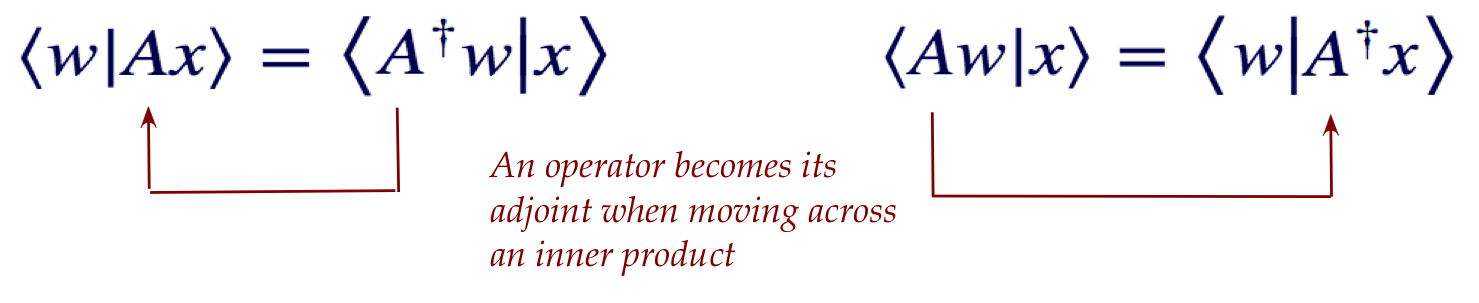
- Recall from earlier, for any operator \(A\) and vectors
\(\kt{w}, \kt{x}\)
$$
\inrs{w}{Ax} \eql \inrs{A^\dagger w}{x}
$$
- For a Hermitian operator, the right side becomes
$$
\inrs{w}{Ax} \eql \inrs{Aw}{x}
$$
- Next, substitute \(w=v, x=v\) to get
$$
\inrs{Av}{v} \eql \inrs{v}{Av}
$$
- Applying the eigenvalue relation on both sides,
$$
\inrs{\lambda v}{v} \eql \inrs{v}{\lambda v}
$$
and factoring out \(\lambda\),
$$
\lambda^* \inr{v}{v} \eql \lambda \inr{v}{v}
$$
- Thus, \(\lambda^* = \lambda\) which makes it real.
Application:
- This turns out to matter when a Hermitian matrix is written
in its eigenbasis, in which case the only non-zero elements
(the eigenvalues) are on the diagonal.
- These eigenvalues correspond to real-world quantities
that are observed (such as energy, for example).
- Proposition 2.7:
Eigenvectors corresponding two distinct eigenvalues
of a Hermitian operator are orthogonal.
Proof:
- Let \(\lambda_1, \lambda_2\) be two distinct eigenvalues
corresponding to eigenvectors \(\kt{v_1}, \kt{v_2}\).
- Then
$$
\inr{Av_1}{v_2} \eql \inr{\lambda_1 v_1}{v_2}
\eql \lambda_1^* \inr{v_1}{v_2}
\eql \lambda_1 \inr{v_1}{v_2}
$$
(The last step because eigenvalues are real.)
- Next,
$$
\inrs{v_1}{Av_2} \eql \inrs{v_1}{\lambda_2 v_2}
\eql \lambda_2 \inr{v_1}{v_2}
$$
- Then, \(\lambda_1 \inr{v_1}{v_2} = \lambda_2 \inr{v_1}{v_2}\)
because
$$
\inrs{Av_1}{v_2} \eql \inrs{v_1}{A^\dagger v_2}
\eql \inrs{v_1}{A v_2}
$$
since \(A = A^\dagger\).
- Thus, subtracting
$$
(\lambda_1 - \lambda_2) \inr{v_1}{v_2} \eql 0
$$
Which means \(\inr{v_1}{v_2} = 0\) since the eigenvalues
are assumed to be distinct.
Application:
- This is critical in quantum mechanics because of the
way measurements work (as we'll see). When a measurement
results one of two different eigenvalues, the resulting
state (an eigenvector) will be exactly one or the other.
- In quantum computing, we will exploit this to reason about
Hermitians.
- Proposition 2.8: (The spectral theorem for
Hermitian operators)
A Hermitian operator \(A\) on an n-dimensional
vector space \(V\) has \(n\) orthonormal eigenvectors
\(\kt{v_1},\ldots,\kt{v_n}\)
with eigenvalues \(\lambda_1,\ldots,\lambda_n\)
such that:
- \(\kt{v_1},\ldots,\kt{v_n}\) form a basis for \(V\).
- \(A\) is a diagonal matrix
$$
\mat{\lambda_1 & 0 & 0 & 0 \\
0 & \lambda_2 & 0 & 0 \\
\vdots & 0 & \ddots & 0 \\
0 & 0 & 0 & \lambda_n
}
$$
when written in the basis \(\kt{v_1},\ldots,\kt{v_n}\).
- \(A = \sum_{i=1}^n \lambda_i \otr{v_i}{v_i}\).
Proof:
The proof is somewhat long and uses induction;
we'll refer you to Axler's book.
- Let's illustrate part-(iii), \(A = \sum_{i=1}^n \lambda_i
\otr{v_i}{v_i}\), with an example:
- Consider the Hermitian (all real-valued, in this case):
$$
A \eql \mat{2 & 1\\ 1 & 2}
$$
with eigenvalues \(\lambda_1 = 1, \lambda_2 = 3\) and
normalized eigenvectors
$$
\kt{v_1} \eql \mat{ \isqt{1} \\ - \isqt{1} }
\;\;\;\;\;\;\;\;
\kt{v_2} \eql \mat{ \isqt{1} \\ \isqt{1} }
$$
where
$$
A\kt{v_1} \eql \mat{2 & 1\\ 1 & 2} \; \mat{ \isqt{1} \\ - \isqt{1} }
\eql 1 \; \mat{ \isqt{1} \\ - \isqt{1} } \eql \lambda_1 \kt{v_1}
$$
and
$$
A\kt{v_2} \eql \mat{2 & 1\\ 1 & 2} \; \mat{ \isqt{1} \\ \isqt{1} }
\eql 3 \; \mat{ \isqt{1} \\ \isqt{1} } \eql \lambda_2 \kt{v_2}
$$
as one would expect.
- Now let's calculate
$$\eqb{
\lambda_1 \otr{v_1}{v_1} \; + \lambda_2 \otr{v_2}{v_2}
& \eql &
1 \mat{ \isqt{1} \\ - \isqt{1} } \mat{ \isqt{1} & - \isqt{1} }
\;\; + \;\;
3 \mat{ \isqt{1} \\ \isqt{1} } \mat{ \isqt{1} & \isqt{1} } \\
& \eql &
\frac{1}{2} \mat{1 & -1\\ -1 & 1}
\;\; + \;\;
\frac{3}{2} \mat{1 & 1\\ 1 & 1} \\
& \eql &
\mat{2 & 1\\ 1 & 2} \\
& \eql & A
}$$
2.11
Useful properties: orthonormality and projector operators
Squared amplitudes add up to 1:
Projectors and Hermitians:
- Proposition 2.10:
A projector is idempotent. That is,
$$
P_v^2 = P_v
$$
so that when a projector is applied twice in succession
the same result obtains.
Proof:
$$\eqb{
P_v^2 & \eql & P_v P_v & \\
& \eql & \otr{v}{v} \: \otr{v}{v}
& \mbx{Each projector is an outer-product}\\
& \eql & \kt{v} \left( \inr{v}{v} \right) \br{v}
& \mbx{Associativity} \\
& \eql & \kt{v} \times 1 \times \br{v}
& \mbx{Inner-product} \\
& \eql & \otr{v}{v} & \\
& \eql & P_v
}$$
Application: this matches intuition
- When we project a vector \(\kt{u}\) onto \(\kt{v}\),
we get a vector along \(\kt{v}\).
- Suppose we call that vector \(\kt{y} = P_v\kt{u}\).
- Applying \(P_v\) twice is the same as applying \(P_v\)
to \(\kt{y}\), i.e., \(P_v P_v \kt{u} = P_v \kt{y}\).
- But the projection of a vector that's already along
\(\kt{v}\) leaves the vector unchanged.
- Thus, \(P_v \kt{y} = \kt{y}\).
- Which means \(P_v P_v \kt{u} = P_v\kt{u}\) or
\(P_v^2 = P_v\)
- Proposition 2.11:
A projector is Hermitian. That is, the projector
\(P_v = \otr{v}{v}\) satisfies \(P^\dagger = P\).
Proof:
See earlier exercise.
Application:
We will see a stronger result below, but we'll need this one
when projectors need to be combined for multiple qubits.
- Proposition 2.12:
The projector \(P_v = \otr{v}{v}\) has eigenvector \(\kt{v}\)
with eigenvalue \(1\).
Proof:
Clearly
$$
P_v\kt{v} \eql \otr{v}{v} \: \kt{v}
\eql \kt{v} \: \inr{v}{v}
\eql \kt{v}
$$
- Proposition 2.13:
For real number \(\lambda\) and projector \(P_v = \otr{v}{v}\),
the operator \(\lambda P_v\) is Hermitian with
eigenvector \(\kt{v}\) and eigenvalue \(\lambda\).
Proof:
The fact that \(\lambda P_v\) is Hermitian follows from the
proposition earlier (Proposition 2.4) that showed that for any real scalar
\(\lambda\) and Hermitian \(A\), the operator \(\lambda A\) is Hermitian.
Next,
$$
(\lambda P_v) \kt{v}
\eql \lambda P_v \kt{v}
\eql \lambda \kt{v}
$$
Which makes \(\kt{v}\) an eigenvector of \(\lambda P_v\)
with eigenvalue \(\lambda\).
- Proposition 2.14:
Let \(P_{v_1},\ldots,P_{v_n}\) be projectors for orthonormal basis
vectors \(\kt{v_1},\ldots,\kt{v_n}\). Next, let
\(\lambda_1,\ldots,\lambda_n\) be real numbers.
Then the real linear combination
$$
A \eql \sum_i \lambda_i P_{v_i} \eql \sum_i \lambda_i \otr{v_i}{v_i}
$$
is a Hermitian operator with eigenvectors
\(\kt{v_1},\ldots,\kt{v_n}\) and corresponding
eigenvalues \(\lambda_1,\ldots,\lambda_n\).
Proof:
The previous proposition shows that each \(\lambda_i P_{v_i}\)
is Hermitian. The sum of Hermitians is Hermitian.
Next,
$$
A\kt{v_i} \eql \parenl{ \sum_k \lambda_k P_{v_k} } \kt{v_i}
\eql \lambda_i P_{v_i} \kt{v_i}
\eql \lambda_i \kt{v_i}
$$
Application:
- This is really part-(iii) of
Proposition 2.8 in the opposite direction,
that the linear combination of projectors for any orthobasis (not
necessarily the eigenbasis) is Hermitian.
- This structure will be the key to understanding one of
the most counter-intuitive aspects of quantum computing: measurement.
Let's emphasize this last point a little differently:
- Suppose we have an orthonormal basis \(\kt{v_1},\ldots,\kt{v_n}\).
- Separately, suppose we have a collection of
real numbers \(\lambda_1,\ldots,\lambda_n\).
- Now, construct the projectors
$$
P_{v_i} \eql \otr{v_i}{v_i}
$$
- Then, construct the operator \(A\) as a linear combination
of the projectors using the \(\lambda_i\)'s as coefficients:
$$
A \eql \sum_i \lambda_i P_{v_i} \eql \sum_i \lambda_i \otr{v_i}{v_i}
$$
- If we do this, then
- \(A\) is Hermitian
- \(A\)'s eigenvectors are the \(\kt{v_i}\)'s with
\(\lambda_i\)'s as corresponding eigenvalues.
- Thus, in some sense, \(A\) "packages" the projectors
into a single operator such that one extracts
the original basis as its eigenvectors.
- As we will see later, this is a critically important concept
in how measurement is analyzed.
2.12
Useful properties: unitary operators
Recall:
A unitary operator \(A\) is one that satisfies
\(A^\dagger A = A A^\dagger = I\)
\(\rhd\)
That is, \(A^{-1} = A^\dagger\)
Example:
- Suppose
$$
A \eql \mat{ \frac{1+i}{2} & \frac{1-i}{2}\\
\frac{1-i}{2} & \frac{1+i}{2}\\ }
$$
- Then
$$
A^\dagger \eql \frac{1}{2}
\mat{ 1-i & 1+i\\
1+i & 1-i\\ }
$$
- We see that
$$
A^\dagger A \eql \frac{1}{2}
\mat{ 1-i & 1+i\\
1+i & 1-i\\ }
\frac{1}{2}
\mat{ 1+i & 1-i\\
1-i & 1+i\\ }
\eql \frac{1}{4} \mat{4 & 0\\0 & 4} \eql I
$$
- An aside: we will meet this particular matrix later
as \(A = \sqrt{X}\) where \(X\) is another well-known matrix.
Let's work through some useful properties of unitary operators
- Proposition 2.15:
A unitary operator preserves inner-products:
\(\inr{Au}{Av} = \inr{u}{v}\).
Proof:
We'll exploit the operator-across-inner-product property here:
$$
\inr{Au}{Av}
\eql \inrs{A^\dagger (Au)}{v}
\eql \inrs{(A^\dagger A)u)}{v}
\eql \inrs{Iu}{v}
\eql \inr{u}{v}
$$
- Proposition 2.16:
A unitary operator preserves lengths:
\(|Au| = |u|\).
Proof:
From the above property
$$
|Au|^2 \eql \inrs{Au}{Au} \eql \inr{u}{u} = |u|^2
$$
- Proposition 2.17:
If \(A\) is unitary so are \(A^\dagger\) and \(A^{-1}\).
Proof:
The definition of unitary is symmetric: \(A\)
is unitary if \(A A^\dagger = A^\dagger A = I\).
Thus, \(A^\dagger\) is also unitary, and because
\(A^{-1} = A^\dagger\), it too is unitary.
- Proposition 2.18:
The columns of \(A\) are orthonormal, as are the rows.
Proof:
- Consider the product \(A^\dagger A = I\) and the i-j-th
element of \(I\).
- This is formed by multiplying the i-th row
of \(A^\dagger\) (conjugate of the i-th column) into the j-th
column of \(A\).
- When \(i\neq j\) we get \(0\), meaning the
i and j columns are orthogonal.
- Similarly, when \(i=j\), we
get a diagonal element of \(I\), which is 1,
meaning each column is of unit length.
The argument for orthonormality of the rows uses the
same arguments with \(AA^\dagger = I\).
- Proposition 2.19:
If \(\kt{v_1},\ldots,\kt{v_n}\) are orthonormal,
so are \(\kt{Av_1},\ldots,\kt{Av_n}\) when \(A\) is unitary.
Proof:
What we need to show is that \(\inrs{Av_i}{Av_j} = 0\) if
\(i\neq j\) and \(\inrs{Av_i}{Av_j} = 1\) if \(i=j\).
This follows from the preservation of
inner products: \(\inrs{Av_i}{Av_j} = \inr{v_i}{v_j}\)
- Another way of saying 2.19: a unitary transformation of an
orthonormal basis produces an orthonormal basis.
- Proposition 2.20:
If \(A, B\) are unitary, then so are \(AB\) and \(BA\).
Proof:
$$
(AB)^\dagger \: (AB)
\eql (B^\dagger A^\dagger) \: (AB)
\eql B^\dagger \: (A^\dagger A) \: B
\eql B^\dagger (I) B
\eql B^\dagger B
\eql I
$$
The proof for \(BA\) is similar.
Application:
- The product rule above is probably the most frequently
applied. Think of \(A\) and \(B\) as two gates that occur
in sequence. The net result is the product, as we will see.
- The other properties above are useful in reasoning
about unitary matrices and building the theory.
In-Class Exercise 13:
Use a \(2\times 2\) example to show that
the sum of two unitary matrices is not necessarily unitary.
2.13
The operator sandwich
Let's now return to applying an operator from the left, and from the right:
- We have seen that
$$
A\kt{v} \eql \kt{Av}
$$
and thus there is no ambiguity in writing either way.
- Similarly, when applying from the right:
$$
\br{Au} \eql \br{u} A^\dagger
$$
which means
$$
\br{A^\dagger u} \eql \br{u} A
$$
- Next, consider the expression
$$
\swich{u}{A}{v}
$$
- If \(A\) were applied to the left of \(\kt{v}\),
this would become:
$$
\swich{u}{A}{v} \eql \inrs{u}{Av}
$$
- If \(A\) were applied to the right of \(\br{u}\):
$$
\swich{u}{A}{v} \eql \inrs{A^\dagger u}{v}
$$
- But both result in the same inner product:
$$
\inr{u}{Av} \eql \inrs{A^\dagger u}{v}
$$
- Thus, the actual calculation could be done either
way.
- We will use the so-called operator sandwich to
write this as
$$
\swich{u}{A}{v}
$$
where it's implied that we have two (equivalent) ways of performing the calculation.
- Note:
- \(\swich{u}{A}{v}\) is still an inner-product, and
will result in a number.
- This result applies to any operator, not just Hermitian and
unitary operators.
Let's see how this works through an example:
- Suppose
$$
A \eql \mat{i & 1\\ 1 & -i}
\;\;\;\;\;\;\;
\kt{u} \eql \vectwo{1}{0}
\;\;\;\;\;\;\;
\kt{v} \eql \vectwo{\isqt{1}}{\isqt{1}}
$$
- We'll first calculate
$$\eqb{
\swich{u}{A}{v}
& \eql & \inr{u}{Av} \\
& \eql &
\mat{1 & 0} \; \left(
\mat{i & 1\\ 1 & -i} \vectwo{\isqt{1}}{\isqt{1}}
\right) \\
& \eql &
\mat{1 & 0} \; \vectwo{\isqt{1+i}}{\isqt{1-i}}\\
& \eql &
\isqt{1+i}
}$$
- And now the other way:
$$
\swich{u}{A}{v}
\eql \inrs{A^\dagger u}{v} \\
$$
First, note that
$$
A^\dagger u
\eql \mat{-i & 1\\ 1 & i} \vectwo{1}{0}
\eql \vectwo{-i}{1}
$$
The inner-product of the conjugated row \(\br{A^\dagger u}\) with \(\kt{v}\)
then is
$$
\inr{A^\dagger u}{v}
\eql
\mat{i & 1} \vectwo{\isqt{1}}{\isqt{1}}
\eql
\isqt{1+i}
$$
Which is, as expected, the same result (number) as before.
How it's used:
- The operator sandwich is used frequently and is yet another
notational and conceptual idea we need to get comfortable with.
- Here's one example with a projector:
- Consider the projection of \(\kt{u}\) on \(\kt{v}\).
- We know that the projector is written as the outer-product
$$
P_v \eql \otr{v}{v}
$$
- Now consider the sandwich
$$
\swich{u}{P_v}{u}
\eql
\br{u} \: \otr{v}{v} \: \kt{u}
\eql
\inr{u}{v} \: \inr{v}{u}
\eql
(\inr{v}{u})^* \: \inr{v}{u}
\eql
\magsq{\inr{v}{u}}
$$
- Thus, \(\swich{u}{P_v}{u}\) is the squared
magnitude of the coefficient in the projection.
- Here's another example with projectors:
- The projected vector when projecting \(\kt{u}\)
along \(\kt{v}\) is: \(P_v\kt{u}\).
- Suppose we want the length of this vector: \(\mag{P_v\kt{u}}\).
- We can write the squared magnitude as:
$$\eqb{
\magsq{P_v\kt{u}}
& \eql &
\left( P_v\kt{u} \right)^\dagger \: P_v\kt{u}
& \mbx{Inner product of \(P_v\kt{u}\) with itself} \\
& \eql &
\left( \br{u} P_v^\dagger \right) \: P_v\kt{u}
& \mbx{Apply adjoint} \\
& \eql &
\br{u} P_v \: P_v\kt{u}
& \mbx{A projector is Hermitian} \\
& \eql &
\swich{u}{P_v}{u}
& \mbx{A projector is idempotent} \\
}$$
This is the same as \(\magsq{\inr{v}{u}}\) derived earlier because
we're working with unit-length vectors.
Let's work through a problem to get some practice:
- The problem: compute \(\swich{u}{P_{v_1}}{u}\) given
\(\kt{u} = \alpha \kt{v_1} + \beta \kt{v_2}\).
- Let's start with
$$\eqb{
P_{v_1} \kt{u}
& \eql &
\otr{v_1}{v_1} \: \parenl{ \alpha \kt{v_1} + \beta \kt{v_2} }
& \mbx{Projector as outer-product} \\
& \eql &
\kt{v_1} \: \parenl{ \alpha \inr{v_1}{v_1} + \beta \inr{v_1}{v_2} }
& \mbx{Right-linearity of inner-product} \\
& \eql &
\kt{v_1} \alpha
& \mbx{Basis vector inner-products} \\
& \eql &
\alpha \kt{v_1} &\\
}$$
- Next,
$$\eqb{
\swich{u}{P_{v_1}}{u}
& \eql &
\br{\alpha v_1 + \beta v_2} \: \alpha \kt{v_1}
& \mbx{Sub for \(\kt{u}\) on left, and above-computed \(P_{v_1}\kt{u}\)} \\
& \eql &
\alpha \inr{\alpha v_1 + \beta v_2}{v_1}
& \mbx{Move second \(\alpha\)} \\
& \eql &
\alpha \left(\alpha^* \inr{v_1}{v_1} + \beta^* \inr{v_2}{v_1} \right)
& \mbx{Left-side linearity} \\
& \eql & \alpha \alpha^*
& \mbx{Basis vector inner-products} \\
& \eql & |\alpha|^2 \\
& \eql & |\inr{v_1}{u}|^2
}$$
- This is typically applied as follows:
- \(\kt{v_1}, \kt{v_2}\) will be an orthonormal basis
- \(\kt{u}\) is some (unit-length) vector
- Which means we can write
$$
\kt{u} \eql \alpha \kt{v_1} + \beta \kt{v_2}
$$
- Then, \(\swich{u}{P_{v_1}}{u}\) gives us the squared-magnitude
of the coefficient \(\alpha\).
- Which is also \(|\inr{v_1}{u}|^2\)
In-Class Exercise 14:
Suppose \(A=\mat{2 & 0\\ 0 & 3}\) and
\(\kt{u} = \alpha \kt{e_1} + \beta \kt{e_2}\). Show that
\(\swich{u}{A}{u} = 2|\alpha|^2 + 3|\beta|^2\)
2.14
A key question: what is the basis of the moment?
In the regular linear algebra we've studied:
- We see multiple bases but we typically
only use coordinates from the standard basis.
- We rarely if ever switch coordinates to a non-standard basis.
- And almost never express a matrix in a non-standard basis.
In quantum computing (and mechanics), on the other hand:
- We use different bases at different times.
- It is essential to know at any time which basis
is being used, and for what.
- When using a non-standard basis we have two options:
- Use the non-standard basis but using coordinates from the
standard basis for calculations.
- Convert to the coordinates of the non-standard basis and
then calculate from there.
We'll illustrate both below.
Let's work through an example to clarify:

- We'll use real numbers so that we can draw vectors (above).
- Here, there are two bases shown:
- The standard basis:
$$
\kt{e_1} \eql \vectwo{1}{0}
\;\;\;\;\;\;\;
\kt{e_2} \eql \vectwo{0}{1}
$$
- Another basis (called the Hadamard basis):
$$
\kt{v_1} \eql \vectwo{\isqt{1}}{\isqt{1}}
\;\;\;\;\;\;\;
\kt{v_2} \eql \vectwo{\isqt{1}}{-\isqt{1}}
$$
Because \(\isqt{1}\approx 0.707\), the coordinates are labeled as such.
- Notice that the diagram shows projections of the vector
$$
\kt{u} \eql \vectwo{\frac{\sqrt{3}}{2}}{\frac{1}{2}}
$$
along \(\kt{e_1}\) (in green) and along \(\kt{v_1}\) (in blue).
- Let
$$\eqb{
\kt{y_1} \; \defn \; \mbox{projection along } \kt{e_1} \\
\kt{w_1} \; \defn \; \mbox{projection along } \kt{v_1} \\
}$$
Let's first use standard-basis coordinates for
calculations:
- The projector for \(\kt{e_1}\) is:
$$
P_{e_1} \eql \otr{e_1}{e_1} \eql
\vectwo{1}{0} \mat{1 & 0}
\eql
\mat{1 & 0\\ 0 & 0}
$$
- Then, the projection of \(\kt{u}\) along \(\kt{e_1}\) is:
$$
\kt{y_1} \eql P_{e_1} \kt{u}
\eql
\mat{1 & 0\\ 0 & 0} \vectwo{\frac{\sqrt{3}}{2}}{\frac{1}{2}}
\eql
\vectwo{\frac{\sqrt{3}}{2}}{0}
$$
- The projector for \(\kt{v_1}\) is:
$$
P_{v_1} \eql \otr{v_1}{v_1} \eql
\vectwo{\isqt{1}}{\isqt{1}}
\mat{\isqt{1} & \isqt{1}}
\eql
\mat{\frac{1}{2} & \frac{1}{2}\\
\frac{1}{2} & \frac{1}{2}}
$$
- And therefore the projection of \(\kt{u}\) along \(\kt{v_1}\) is:
$$
\kt{w_1} \eql P_{v_1} \kt{u}
\eql
\mat{\frac{1}{2} & \frac{1}{2}\\
\frac{1}{2} & \frac{1}{2}}
\vectwo{\frac{\sqrt{3}}{2}}{\frac{1}{2}}
\eql
\vectwo{\frac{\sqrt{3}+1}{4}}{\frac{\sqrt{3}+1}{4}}
$$
This should make sense because \(\kt{v_1}\) is at a \(45^\circ\)
angle and so both coordinates should be the same.
- Let's point out:
- Although \(\kt{v_1}, \kt{v_2}\) is a different basis than
\(\kt{e_1}, \kt{e_2}\), all calculations have been done
using coordinates from \(\kt{e_1}, \kt{e_2}\) (standard-basis).
- We know this because \(\kt{v_1}, \kt{v_2}\) themselves
were written in standard-basis coordinates:
$$
\kt{v_1} \eql \vectwo{\isqt{1}}{\isqt{1}}
\;\;\;\;\;\;\;
\kt{v_2} \eql \vectwo{\isqt{1}}{-\isqt{1}}
$$
- Thus, all the calculations have been done in the standard basis.
Now let's see what it's like to perform calculations in the
other basis, the \(\kt{v_1}, \kt{v_2}\) basis:
- First, we'll ask: what are the coordinates of the
basis vectors \(\kt{v_1}, \kt{v_2}\) in their own basis?
- To get the coordinates of \(\kt{v_1}\) in
the \(\kt{v_1}, \kt{v_2}\) basis, we need to solve
$$
\alpha_1 \kt{v_1} + \alpha_2 \kt{v_2} \eql \kt{v_1}
$$
- That is, what linear combination of the basis vectors
gives us the target vector \(\kt{v_1}\), in this case)?
- Clearly, the solution is \(\alpha_1=1, \alpha_2=0\).
- Similarly, to get the coordinates of \(\kt{v_2}\), we solve
$$
\beta_1 \kt{v_1} + \beta_2 \kt{v_2} \eql \kt{v_2}
$$
to get \(\beta_1=0, \beta_2=1\).
- Thus the coordinates of \(\kt{v_1}, \kt{v_2}\) in the new basis
are:
$$
\kt{v_1} \eql \vectwo{1}{0}
\;\;\;\;\;\;\;
\kt{v_2} \eql \vectwo{0}{1}
$$
- Surprised by this (simple) result? We'll have more to say
about this below.
- Next, let's write \(\kt{u}\) in the \(\kt{v_1}, \kt{v_2}\)
basis:
- We need to solve
$$
\gamma_1 \kt{v_1} + \gamma_2 \kt{v_2} \eql \kt{u}
$$
- How do we solve for \(\gamma_1,\gamma_2\) without knowing
\(\kt{u}\)?
- The key insight is that \(\gamma_1,\gamma_2\) will be the
same no matter which basis is used.
- So, since we know \(\kt{u}\) in the standard basis, we'll
first use the standard basis:
That is,
$$
\gamma_1 \vectwo{\isqt{1}}{\isqt{1}}
+ \gamma_2 \vectwo{\isqt{1}}{-\isqt{1}}
\eql
\vectwo{\frac{\sqrt{3}}{2}}{\frac{1}{2}}
$$
- Which we can write in matrix form:
$$
\mat{\isqt{1} & \isqt{1}\\
\isqt{1} & -\isqt{1}}
\vectwo{\gamma_1}{\gamma_2}
\eql
\vectwo{\frac{\sqrt{3}}{2}}{\frac{1}{2}}
$$
- We could solve this the usual linear-equation way, but
notice that the matrix is unitary, which means the inverse
is the adjoint.
- Thus
$$
\kt{u} \eql
\mat{\isqt{1} & \isqt{1}\\
\isqt{1} & -\isqt{1}}
\vectwo{\frac{\sqrt{3}}{2}}{\frac{1}{2}}
\eql
\vectwo{\frac{\sqrt{3}+1}{2\sqrt{2}}}{\frac{\sqrt{3}-1}{2\sqrt{2}}}
$$
- Now that we know the coordinates of \(\kt{u}\) in the
new basis, let's compute the projection along \(\kt{v_1}\):
- The projector in new coordinates is:
$$
P_{v_1} \eql
\otr{v_1}{v_1}
\eql
\vectwo{1}{0} \mat{1 & 0}
\eql
\mat{1 & 0\\ 0 & 0}
$$
- Applying this to \(\kt{u}\):
$$
\kt{w_1} \eql P_{v_1} \kt{u} \eql
\mat{1 & 0\\ 0 & 0}
\vectwo{\frac{\sqrt{3}+1}{2\sqrt{2}}}{\frac{\sqrt{3}-1}{2\sqrt{2}}}
\eql
\vectwo{\frac{\sqrt{3}+1}{2\sqrt{2}}}{0}
$$
- Again, the result should make sense: in the new coordinates,
we expect the projection to be a scalar multiple of \(\kt{v_1}=(1,0)\).
- That scalar in the \(\kt{v_1}, \kt{v_2}\) coordinates is:
$$
\kt{w_1} \eql
\vectwo{\frac{\sqrt{3}+1}{2\sqrt{2}}}{0}
\eql \smm{\frac{\sqrt{3}+1}{2\sqrt{2}}} \vectwo{1}{0}
\eql \smm{\frac{\sqrt{3}+1}{2\sqrt{2}}} \kt{v_1}
$$
- We should of course get the same scalar in the standard coordinates:
$$
\kt{w_1} \eql
\vectwo{\frac{\sqrt{3}+1}{4}}{\frac{\sqrt{3}+1}{4}}
\eql \smm{\frac{\sqrt{3}+1}{2\sqrt{2}}} \vectwo{\isqt{1}}{\isqt{1}}
\eql \smm{\frac{\sqrt{3}+1}{2\sqrt{2}}} \kt{v_1}
$$
In-Class Exercise 15:
Using \(\kt{v_1}, \kt{v_2}\) as the basis,
- Find the coordinates of \(\kt{e_1}, \kt{e_2}\);
- Then, compute \(\kt{y_2} = P_{e_2}\kt{u}\) in this basis.
- Check your calculations by obtaining \(\kt{y_2}\)
in the standard basis and converting that to the
\(\kt{v_1}, \kt{v_2}\) basis.
Let's make a few comments about bases:
- Let's start by asking: when do we exercise a choice in basis?
- There are only two reasons to use a particular basis:
- When the use of the basis is part of the design:
- This occurs when we seek a particular outcome from a
particular basis.
- When a different basis makes calculations easier, and
insight possible.
- Most often, the first reason will drive our choices.
- That is, we'll do calculations in the standard basis.
- But we'll want projections and such onto vectors in a
non-standard basis.
- We'll calculate these projections with standard-basis coordinates.
- It's equally important to understand that much of the
theory does not need a choice of basis to be made when proving a result.
- To see why, let's go back to our projection picture:
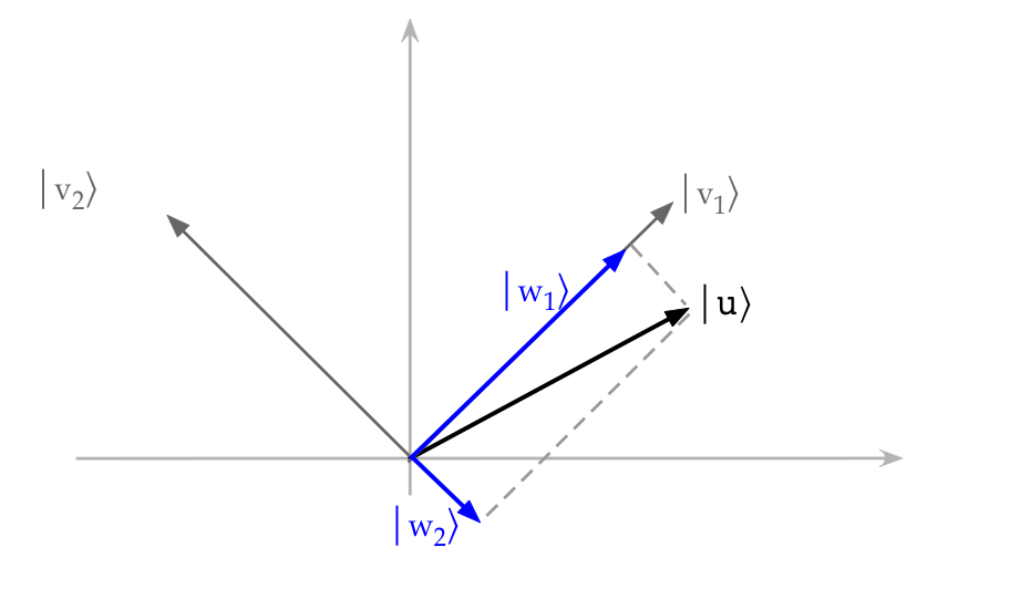
- Here, the (real) vectors are abstract "arrows".
- We "numerify" an arrow when an arrow is written in
terms of basis vectors.
- For example:
$$
\kt{u} \eql
\smm{\frac{\sqrt{3}}{2}} \vectwo{1}{0}
+ \smm{\frac{1}{2}} \vectwo{0}{1}
\eql
\vectwo{\frac{\sqrt{3}}{2}}{\frac{1}{2}}
$$
This provides coordinates in the chosen basis (the standard
basis in this case).
- Next, observe that
- The notion of projection can be
described geometrically (for real vectors) without
any reference to which basis vectors.
- More valuably, the notion of projection can be described
algebraically without reference to a basis, that is,
without "numerifying".
- For example, the projection of \(\kt{u}\) along \(\kt{v_1}\) is just
$$
\otr{v_1}{v_1} \: \kt{u}
$$
whichever basis is used.
- What is (mathematically) interesting is that:
- Much of the theory can be laid out in a basis-free manner.
- And, in fact, can be proved for more general and abstract
forms of vectors.
- For example: functions.
- One defines a vector space as a set of mathematical objects
that satisfy certain rules like addition, scalar multiplication
and so on.
- Certainly, the vectors we've seen satisfy this definition.
- But so do functions, which allows the theory to apply more broadly.
- To perform calculations (numbers!) we of course need to use some
basis.
- The choice of basis is often up to us.
2.15
Getting used to Dirac notation
Because we will see certain Dirac symbols and notation repeatedly,
let's revisit parts of the previous section in this
notation:
- First, we'll relabel the picture
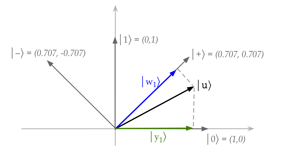
- Next, the standard basis vectors are written as
$$\eqb{
\kt{0} & \eql & \vectwo{1}{0} \\
\kt{1} & \eql & \vectwo{0}{1}
}$$
- The second basis is called the Hadamard basis and
is written as:
$$\eqb{
\kt{+} & \eql & \vectwo{\isqt{1}}{\isqt{1}}\\
\kt{-} & \eql & \vectwo{\isqt{1}}{-\isqt{1}}
}$$
- Observe that
$$\eqb{
\kt{+} & \eql & \vectwo{\isqt{1}}{\isqt{1}}
\eql \smm{\isqt{1}} \vectwo{1}{0} + \smm{\isqt{1}} \vectwo{0}{1}
\eql \smm{\isqt{1}} \kt{0} + \smm{\isqt{1}} \kt{1} \\
\kt{-} & \eql & \vectwo{\isqt{1}}{-\isqt{1}}
\eql \smm{\isqt{1}} \vectwo{1}{0} - \smm{\isqt{1}} \vectwo{0}{1}
\eql \smm{\isqt{1}} \kt{0} - \smm{\isqt{1}} \kt{1} \\
}$$
- The projector for \(\kt{0}\) is:
$$
P_{0} \eql \otr{0}{0} \eql
\vectwo{1}{0} \mat{1 & 0}
\eql
\mat{1 & 0\\ 0 & 0}
$$
And the projector for \(\kt{1}\) is:
$$
P_{1} \eql \otr{1}{1} \eql
\vectwo{0}{1} \mat{0 & 1}
\eql
\mat{0 & 0\\ 0 & 1}
$$
- Similarly, the projector for \(\kt{+}\) is:
$$
P_{+} \eql \otr{+}{+} \eql
\vectwo{\isqt{1}}{\isqt{1}}
\mat{\isqt{1} & \isqt{1}}
\eql
\mat{\frac{1}{2} & \frac{1}{2}\\
\frac{1}{2} & \frac{1}{2}}
$$
In-Class Exercise 16:
This is just a writing exercise to get used to
the new symbols. Rewrite the previous exercise
with the new symbols. That is,
using \(\kt{+}, \kt{-}\) as the basis,
- Find the coordinates of \(\kt{0}, \kt{1}\);
- Then, compute \(\kt{y_2} = P_{1}\kt{u}\) in this basis.
- Check your calculations by obtaining \(\kt{y_2}\)
in the standard basis and converting that to the
\(\kt{+}, \kt{-}\) basis.
2.16*
Operator-matrix and change-of-basis via sandwich and inner product
We'll now work through two useful results:
- If an operator is not in matrix form, then how do we obtain its matrix?
- How do we change coordinates from one basis to another?
Although we've seen the second one before (in the Review), we'll
use our newfound approach with the operator sandwich, and inner
products.
And at the end, we'll explain why this is a powerful tool.
Let's start with the matrix of an operator:
- This may seem an odd objective because ... aren't all operators
already matrices?
- In fact, no. An operator can be specified by text
description.
- For example, let \(A\) be the operator that multiplies
any 2D vector element by 3:
$$
A \kt{\psi} \eql 3 \kt{\psi}
$$
- It turns out, in this case, the matrix is:
$$
A \eql \mat{3 & 0\\ 0 & 3}
$$
This is called the matrix representation of the operator \(A\).
- What we seek: a systematic way to obtain the matrix
representation.
- What we also seek: to directly obtain the matrix of an
operator in a given basis.
- We'll do both with this powerful result:
- Suppose \(\kt{v_1},\ldots,\kt{v_n}\) is the desired basis
in which we want the matrix for operator \(A\).
- Define the numbers
$$
A_{ij} \; \defn\; \swich{v_i}{A}{v_j}
$$
- Then the matrix for \(A\) is simply the matrix with
$$
A_{ij} \eql \mbox{element in row i, column j}
$$
- Proposition 2.21:
The matrix of an operator \(A\) in an orthonormal basis
\(\kt{v_1},\ldots,\kt{v_n}\) is formed by elements
\(A_{ij} \defn \swich{v_i}{A}{v_j}\) in row i and column j.
Proof:
We'll do this in two steps:
- First show that the matrix
$$
\hat{A} \; \defn \; \sum_{i,j} A_{ij} \otr{v_i}{v_j}
$$
produces the same effect as the operator \(A\).
- Then show that the i-j-th element of \(\hat{A}\) is
in fact \(\swich{v_i}{A}{v_j}\).
Let's start with the first step:
- First, suppose
$$
\kt{\phi} \eql A \kt{\psi}
$$
for two vectors \(\kt{\psi}\) and \(\kt{\phi}\).
-
Then, express both in the basis:
$$\eqb{
\kt{\psi} \eql \alpha_1 \kt{v_1} + \ldots + \alpha_n \kt{v_n}\\
\kt{\phi} \eql \beta_1 \kt{v_1} + \ldots + \beta_n \kt{v_n}\\
}$$
where \(\alpha_1,\ldots,\alpha_n\) and \(\beta_1,\ldots,\beta_n\)
are the coordinates, respectively, of each of these vectors.
- Now, any outer-product like \(\otr{v_i}{v_j}\) is a matrix and so
$$
\hat{A} \eql \sum_{i,j} A_{ij} \otr{v_i}{v_j}
$$
which is a linear combination of matrices is a matrix.
- Let's apply this matrix to \(\kt{\psi}\):
$$\eqb{
\hat{A} \kt{\psi}
& \eql &
\left( \sum_{i,j} A_{ij} \otr{v_i}{v_j} \right)
\left( \sum_k \alpha_k \kt{v_k} \right) \\
& \eql &
\sum_i \sum_j \sum_k \alpha_k A_{ij} \otr{v_i}{v_j}\: \kt{v_k}\\
& \eql &
\sum_i \sum_j \sum_k \alpha_k A_{ij} \kt{v_i} \: \inr{v_j}{v_k}\\
& \eql &
\sum_i \sum_j \alpha_j A_{ij} \kt{v_i} \\
}$$
where the last simplification comes from the orthonormality
simplification of the inner-products (the case \(j=k\) and \(j\neq k\)).
- Next, write this last expression as
$$
\sum_i \left( \sum_j A_{ij} \alpha_j \right) \kt{v_i}
$$
Now observe: the sum inside the parentheses is the product
of the i-th row of \(\hat{A}\) and \(\kt{\psi}\)
- Recall that
$$
\kt{\phi} \eql \beta_1 \kt{v_1} + \ldots + \beta_n \kt{v_n}\\
$$
and now compare
$$
\kt{\phi} \eql A \kt{\psi}
$$
with what we just derived
$$
\hat{A} \kt{\psi} \eql
\sum_i \left( \sum_j A_{ij} \alpha_j \right) \kt{v_i}
$$
- Because coefficients in a linear combination of basis
vectors are unique,
$$
\beta_i \eql \left( \sum_j A_{ij} \alpha_j \right)
$$
- And thus, the matrix \(\hat{A}\) produces the same
transformation as the operator \(A\).
Next, for step 2, let's ask: in using \(\hat{A}\) for \(A\),
do we get the i-j-th element as \(\swich{v_i}{A}{v_j}\)?
- Consider \(\swich{v_i}{A}{v_j}\).
- Substitute the matrix \(\hat{A}\):
$$\eqb{
\swich{v_i}{\hat{A}}{v_j}
& \eql &
\swichh{v_i}{\sum_{m,n} A_{m,n} \otr{v_m}{v_m}}{v_j} \\
& \eql &
\swichh{v_i}{\sum_{m} A_{m,j} }{v_m} \\
& \eql &
A_{ij} \\
& \eql &
\swich{v_i}{A}{v_j}
}$$
- So, the i-j-th element of \(\hat{A}\) is in fact
\(\swich{v_i}{A}{v_j}\).
Next, we'll see that a change-of-basis matrix can be written
entirely with inner-products:
- Proposition 2.22:
Let \(\kt{v_1},\ldots,\kt{v_n}\) (v-basis) and
\(\kt{w_1},\ldots,\kt{w_n}\) (w-basis) be two bases and suppose that
vector \(\kt{\psi}\) has coordinates \(\alpha_1,\ldots,\alpha_n\)
in the v-basis and coordinates \(\beta_1,\ldots,\beta_n\)
in the w-basis. Then, the matrix with elements
$$
U_{ij} \eql \inr{w_i}{v_j}
$$
converts coordinates from the v-basis to the w-basis. That is,
$$
\vecthree{\beta_1}{\vdots}{\beta_n}
\eql
\mat{ \inr{w_1}{v_1} & \cdots & \inr{w_1}{v_n} \\
\vdots & \vdots & \vdots \\
\inr{w_n}{v_1} & \cdots & \inr{w_n}{v_n} }
\vecthree{\alpha_1}{\vdots}{\alpha_n}
$$
Proof:
First note that the coordinates (coefficients) can be written as:
$$\eqb{
\alpha_i & \eql & \inr{v_i}{\psi} \\
\beta_i & \eql & \inr{w_i}{\psi} \\
}$$
Next, in the matrix-vector product above, consider the k-th row
times the vector \(\ksi\):
$$\eqb{
& \; &
\inr{w_k}{v_1} \alpha_1 + \ldots + \inr{w_k}{v_n} \alpha_n & \\
& \; &
\eql \inr{w_k}{v_1}\: \inr{v_1}{\psi} + \ldots + \inr{w_k}{v_n}
\inr{v_n}{\psi}
& \mbx{Sub for \(\alpha_i\)} \\
& \; &
\eql \swichh{w_k}{ \sum_i \otr{v_1}{v_1} }{\psi}
& \mbx{Associativity} \\
& \; &
\eql \swichs{w_k}{I}{\psi}
& \mbx{Completeness} \\
& \; &
\eql \beta_k
& \\
}$$
Which is indeed the k-th coordinate in the w-basis.
Whew! Both were detailed multi-step proofs that required
careful attention to sums.
Why is this approach useful?
- First, it's practically useful in calculations, as we'll see
below.
- Second, it's useful when we only have
operator descriptions (as opposed to matrices).
Let's apply what we've learned above:
- Example 1: Consider the operator that multiplies
any 2D vector element by 3:
$$
A \kt{\psi} \eql 3 \kt{\psi}
$$
- The first thing to observe is that any matrix that multiplies
basis vectors by 3 will also multiply any vector by three.
- This means, if we use the approach for deriving the matrix
with basis vectors, it'll apply to all vectors (as desired).
-
Let's derive the matrix using \(A_{ij} = \swich{v_i}{A}{v_j}\)
using the standard basis \(\kt{0}, \kt{1}\):
$$
\mat{ \swich{0}{A}{0} & \swich{0}{A}{1}\\
\swich{1}{A}{0} & \swich{1}{A}{1}}
\eql
\mat{ 3\inr{0}{0} & 3\inr{0}{1} \\
3\inr{0}{1} & 3\inr{1}{1} }
\eql
\mat{ 3 & 0\\
0 & 3}
$$
- Consider how we obtained the first element (top left),
\(\swich{0}{A}{0}\):
- First, apply \(A\) to its right: \(A\kt{0} = 3\kt{0}\).
(We know this from the description of \(A\).)
- This results in \(\swich{0}{A}{0} = \br{0}3\kt{0} =
3\inr{0}{0}\).
- Now check that it works for all vectors \(\ksi=\alpha\kt{0} + \beta\kt{1}\):
$$
A \ksi \eql
\mat{ 3 & 0\\
0 & 3}
\vectwo{\alpha}{\beta}
\eql
\vectwo{3 \alpha}{3 \beta}
\eql
3 \ksi
$$
Which it does.
- Example 2:
Let's write the coordinate conversion matrix going from the
standard to the Hadamard basis:
- Recall the Hadamard basis:
$$\eqb{
\kt{+} & \eql & \isqt{1} \kt{0} + \isqt{1} \kt{1} \\
\kt{-} & \eql & \isqt{1} \kt{0} - \isqt{1} \kt{1}
}$$
Note that, from this, we get
$$\eqb{
\br{+} & \eql & \isqt{1} \br{0} + \isqt{1} \br{1} \\
\br{-} & \eql & \isqt{1} \br{0} - \isqt{1} \br{1}
}$$
- Next, the four inner products that will result in
elements of the conversion matrix:
$$\eqb{
\inr{+}{0}
& \eql &
\inrh{ \isqt{1} \br{0} + \isqt{1} \br{1} }{0}
& \eql &
\isqt{1} \inr{0}{0} + \isqt{1} \inr{1}{0}
& \eql & \isqt{1} \\
\inr{+}{1}
& \eql &
\inrh{ \isqt{1} \br{0} + \isqt{1} \br{1} }{1}
& \eql &
\isqt{1} \inr{0}{1} + \isqt{1} \inr{1}{1}
& \eql & \isqt{1} \\
\inr{-}{0}
& \eql &
\inrh{ \isqt{1} \br{0} - \isqt{1} \br{1} }{0}
& \eql &
\isqt{1} \inr{0}{0} - \isqt{1} \inr{1}{0}
& \eql & \isqt{1} \\
\inr{-}{1}
& \eql &
\inrh{ \isqt{1} \br{0} - \isqt{1} \br{1} }{1}
& \eql &
\isqt{1} \inr{0}{1} - \isqt{1} \inr{1}{1}
& \eql & - \isqt{1} \\
}$$
- Thus, the change-of-basis matrix is:
$$
U \eql
\mat{ \inr{+}{0} & \inr{+}{1}\\
\inr{-}{0} & \inr{-}{1}}
\eql
\mat{ \isqt{1} & \isqt{1}\\
\isqt{1} & -\isqt{1}}
$$
Which matches what we saw earlier.
In-Class Exercise 17:
Suppose \(A\) is an operator that "flips" the Hadamard
basis vectors. That is, \(A\kt{+} = \kt{-}\) and
\(A\kt{-} = \kt{+}\). Use the approach above to
derive the matrix for \(A\) in the \(\kt{+},\kt{-}\) basis.
Then, apply the matrix to \(\ksi=\alpha\kt{0} + \beta\kt{1}\).
Is the resulting vector orthogonal to \(\ksi\)?
Finally, let's reiterate how change-of-basis works for
matrices:
If this change-of-basis stuff seems a bit confusing and a bit much
to absorb at one go ... that's because it is so.
2.17
Orthogonal subspaces
Let's return to the idea of a vector space:
- Suppose \(\kt{v_1},\ldots,\kt{v_n}\) is an orthonormal basis
for n-component complex vectors.
- The set
$$\eqb{
V & \eql &
\mbox{span}\setl{\kt{v_1}, \kt{v_2}, \ldots, \kt{v_n}} \\
& \eql &
\setl{ \alpha_1 \kt{v_1} + \alpha_2 \kt{v_2} + \ldots + \alpha_k\kt{v_n}:
\alpha_i \in \mathbb{C} }
}$$
is a vector space, meaning that all linear combinations of
any subset of vectors in \(V\) is in \(V\).
- Another way of saying this: \(V\) is closed under
linear combinations.
- Now consider just the span of the first two of these vectors:
$$\eqb{
W & \eql & \mbox{span}\setl{ \kt{v_1}, \kt{v_2} } \\
& \eql &
\setl{ \alpha_1 \kt{v_1} + \alpha_2 \kt{v_2}:
\alpha_i \in \mathbb{C} }
}$$
Is this a vector space? Let's test:
- Let's, for example, pick three vectors in \(W\) and ask if
the linear combination is in \(W\):
$$\eqb{
\kt{x_1} & \eql & a_1 \kt{v_1} + a_2 \kt{v_2} \\
\kt{x_2} & \eql & b_1 \kt{v_1} + b_2 \kt{v_2} \\
\kt{x_3} & \eql & c_1 \kt{v_1} + c_2 \kt{v_2} \\
}$$
- A linear combination of these three is:
$$
\kt{z} \eql \beta_1 \kt{x_1} + \beta_2 \kt{x_2} + \beta_3 \kt{x_3}
$$
- We want to ask: is \(\kt{z} \in W\)?
- The exercise below shows that it does.
- Observe:
- Every vector in \(W\) is in \(V\).
- Not every vector in \(V\) is in \(W\).
Thus, we say \(W\) is a subspace of \(V\).
- Now consider the set \(W^\prime\):
$$
W^\prime \eql \mbox{span}\setl{ \kt{v_3}, \ldots, \kt{v_n} } \\
$$
One can see that \(W^\prime\) is also a subspace of \(V\).
- Now, there's a complementary relationship between
\(W\) and \(W^\prime\):
- Suppose \(\kt{x}\in W\) and \(\kt{y}\in W^\prime\).
- Then we can use the basis vectors to express them:
$$\eqb{
\kt{x} & \eql & a_1 \kt{v_1} + a_2 \kt{v_2}\\
\kt{y} & \eql & a_3 \kt{v_3} + \ldots + a_n \kt{v_n}\\
}$$
- Then
$$\eqb{
\inr{x}{y} & \eql &
\inrh{ a_1^* \br{v_1} + a_2^* \br{v_2} }{ a_3 \kt{v_3} + \ldots
+ a_n \kt{v_n} } \\
& \eql & 0
}$$
because the \(\kt{v_i}\)'s are orthogonal.
- Thus, every vector in \(W\) is orthogonal to
every vector in \(W^\prime\).
- Two subspaces that satisfy this property are said to
be orthogonal complements:
- We use the notation \(W^\perp = \) orthogonal complement
subspace to \(W\).
- Here, \(W^\perp = W^\prime\)
- Notice also that
$$
W \cup W^\prime \eql V
$$
That is, if we pull into one set every vector in each of \(W,
W^\prime\) we'll get all the vectors in \(V\).
- This notion can extend to multiple subspaces:
- For example, suppose \(W_3=\mbox{span}\setl{\kt{v_3}},
W_4=\mbox{span}\setl{\kt{v_4}},\ldots, W_n=\mbox{span}\setl{\kt{v_n}}\)
- Then any two of these are orthogonal, and all of them
are orthogonal to \(W=\mbox{span}\setl{\kt{v_1},\kt{v_2}}\).
- And
$$
W \cup W_3 \cup \ldots \cup W_n \eql V
$$
In-Class Exercise 18:
Show that \(\kt{z} \in W\).
Projectors for subspaces:
- Recall the definitions of \(V\) and \(W\) from above:
$$\eqb{
V & \eql &
\mbox{span}\setl{ \kt{v_1}, \kt{v_2}, \ldots, \kt{v_n} } \\
W & \eql & \mbox{span}\setl{ \kt{v_1}, \kt{v_2} } \\
}$$
- Let's pick a generic vector in \(V\) from above:
$$
\kt{u} \eql a_1 \kt{v_1} + a_2 \kt{v_2} + \ldots + a_n \kt{v_n}
$$
- Define the matrix
$$\eqb{
P_{v_1,v_2} & \eql & P_{v_1} + P_{v_2}
& \mbx{Projectors for each of \(\kt{v_1}, \kt{v_2}\)}\\
& \eql & \otr{v_1}{v_1} + \otr{v_2}{v_2}
& \mbx{Each projector is an outer-product}\\
}$$
- Let's apply this to the vector \(\kt{u}\):
$$\eqb{
P_{v_1,v_2} \kt{u}
& \eql &
\parenl{ \otr{v_1}{v_1} + \otr{v_2}{v_2} } \;
\parenl{ a_1 \kt{v_1} + a_2 \kt{v_2} + \ldots + a_n \kt{v_n} }\\
& \eql &
\parenl{ \: a_1 \kt{v_1}\: {\bf \inr{v_1}{v_1}} + a_2 \kt{v_1}\: \inr{v_1}{v_2}
+ \ldots + a_n \kt{v_1}\: \inr{v_1}{v_n} \: }\\
& & \; + \;
\parenl{ \: a_1 \kt{v_1}\: \inr{v_2}{v_1} + a_2 \kt{v_1}\: {\bf\inr{v_2}{v_2}}
+ \ldots + a_n \kt{v_1}\: \inr{v_2}{v_n} \: } \\
& \eql &
a_1 \kt{v_1} + a_2 \kt{v_2}
}$$
(Only the two bolded inner products are non-zero.)
- The result is a vector in \(W\).
- This is called the projection of \(\kt{u}\) onto the subspace \(W\).
- In this way, if \(S \subset V\) is any subspace of \(V\),
with basis \(\kt{s_1},\kt{s_2},\ldots,\kt{s_k}\), then the projector
for this subspace is:
$$
P_S \eql \otr{s_1}{s_2} + \ldots + \otr{s_k}{s_k}
$$
This means that if \(\kt{u}\in V\) is any vector in \(V\), the
vector \(P_S \kt{u} \in S\).
- Important: the projected vectors are not necessarily unit-length.
- Example:
- Suppose \(V = \mbox{span}\setl{ \kt{0}, \kt{1} }\).
- Let \(S = \mbox{span} \setl{ \kt{0} }\) be a subspace.
- Then the projector is \(P_S = \otr{0}{0}\).
- Let
$$
\kt{u} \eql \isqts{1} \kt{0} + \isqts{1} \kt{1}
$$
be a vector in \(V\).
- Then
$$\eqb{
P_S \kt{u} & \eql & \otr{0}{0}
\left(\isqts{1} \kt{0} + \isqts{1} \kt{1} \right)
& \mbx{Apply projector} \\
& \eql &
\isqts{1} \kt{0} \: \inr{0}{0} + \isqts{1} \kt{0} \: \inr{0}{1}
& \mbx{Projector distributes} \\
& \eql & \isqts{1} \kt{0}
& \mbx{Associativity groups inner-products} \\
}$$
(Recall: \(\otr{0}{1} = 0\)).
- Then the length of this result is:
$$
\mag{P_S \kt{u}} \eql \mag{ \isqts{1} \kt{0} } \eql \isqts{1}
$$
- Why are projectors important?
- Projectors are how the critical action of measurement
occurs in quantum computing (and mechanics).
- A stronger understanding of this part of the theory makes it
less mysterious than it first appears to be.
- Next, let's work through an example:
- Recall
$$
\kt{+} = \isqts{1} \kt{0} + \isqts{1} \kt{1}
$$
- Let's apply the projector for \(\mbox{span} \setl{ \kt{+} }\)
to the vector \(\kt{0}\).
- First, the projector:
$$
P_+ \eql \vectwo{ \isqt{1} }{ \isqt{1} } \mat{ \isqt{1} & \isqt{1} }
\eql
\mat{ \frac{1}{2} & \frac{1}{2}\\
\frac{1}{2} & \frac{1}{2}}
$$
- Now apply to \(\kt{0}\):
$$
P_+ \kt{0} \eql
\mat{ \frac{1}{2} & \frac{1}{2}\\
\frac{1}{2} & \frac{1}{2}}
\vectwo{1}{0}
\eql
\vectwo{ \frac{1}{2} }{ \frac{1}{2} }
\eql
\isqts{1} \kt{+}
$$
In-Class Exercise 19:
Write down the projector \(P_{-}\) for the subspace
\(\mbox{span}(\kt{-})\).
- Show that \(P_{-} \kt{0} = \isqt{1} \kt{-}\)
- What is the result of applying \(P_{-}\) to \(\kt{+}\)?
The special case of 2D:
- Consider the 2D vector \(\kt{0}\).
- Let's ask: which unit-length 2D vectors \(\kt{w^\perp}\) are
orthogonal to \(\kt{w}=\kt{0}\)?
- Write
$$
\kt{w^\perp} = \alpha \kt{0} + \beta \kt{1}
$$
in terms of the standard basis.
- For orthogonality,
$$\eqb{
& & \inrs{0}{w^\perp} \eql 0 \\
& \implies & \inrh{0}{\alpha \kt{0} + \beta \kt{1}} \eql 0\\
& \implies & \inrh{0}{\alpha \kt{0} + \beta \kt{1}} \eql 0\\
& \implies & \alpha = 0 \\
& \implies & \kt{w^\perp} = \beta \kt{1}\\
}$$
- For unit-length, we must have
$$\eqb{
& \inr{w^\perp}{w^\perp} & \eql & 1\\
\implies & \inrh{\beta^* \br{1}}{\beta\kt{1}} & \eql & 1 \\
\implies & \beta^*\beta \inr{1}{1} & \eql & 1 \\
\implies & \mag{\beta} \eql 1
}$$
- Thus, \(\beta\) can be any complex number of unit magnitude.
- Example: \(\beta=1\)
\(\rhd\)
\(\kt{w^\perp} = \kt{1}\)
- Notice that all the vectors orthogonal to \(\kt{w}=\kt{0}\) are
along \(\kt{w^\perp}=\kt{1}\).
- In some sense, there's only one vector along which lie
the orthogonal vectors to \(\kt{w}=\kt{0}\).
- This is not true for 3D and higher:
- For example, with real vectors, consider \(\kt{w}=(1,0,0)\)
in 3D.
- Any vector in the y-z plane is perpendicular (orthogonal) to
\(\kt{w}\).
- And there are an infinite number of them in an infinite
number of directions.
- When working with single qubits, this observation will be
useful, so let's generalize and observe the following:
- Suppose \(\kt{v}\) and \(\kt{v^\perp}\) are two basis
vectors for 2D.
- Let \(\kt{w} = a\kt{v} + b\kt{v^\perp}\)
- Then \(\kt{w^\perp} = b^*\kt{v} - a^* \kt{v^\perp}\)
is orthogonal because
$$\eqb{
\inr{w}{w^\perp} & \eql &
\inrh{ a^*\br{v} + b^*\br{v^\perp} }{ b^*\kt{v} - a^* \kt{v^\perp} }\\
& \eql &
a^* b^* \inr{v}{v} - b^* a^* \inr{v^\perp}{v^\perp}\\
& \eql &
0
}$$
In-Class Exercise 20:
Suppose
\(\kt{w} = \frac{\sqrt{3}}{2} \kt{0} - \frac{1}{2} \kt{1}\).
- Show that
\(\kt{w^\perp} = \frac{1}{2} \kt{0} + \frac{\sqrt{3}}{2} \kt{1}\)
is orthogonal and of unit-length.
- Express \(\kt{+}\) in this basis by computing the
coefficients \(\inr{w}{+}\) and \(\inr{w^\perp}{+}\).
- Check your calculations by showing
\(\magsq{\inr{w}{+}} + \magsq{\inr{w^\perp}{+}} = 1\).
In-Class Exercise 21:
- Write down the two projectors \(P_0, P_1\) for \(\kt{0}, \kt{1}\),
respectively. Then compute the matrix product \(P_0 P_1\).
- Write down the two projectors \(P_+, P_{-}\) for \(\kt{+}, \kt{-}\),
respectively. Then compute the matrix product \(P_+ P_{-}\).
Explain the resulting product matrices.
2.18*
A mathematical aside
For the theoretically inclined, we'll point out a few things,
none of which are essential to the course but which might
stimulate further curiosity:
- All the theory laid out in this module was done so with
complex vectors and matrices.
- The theory of vector spaces and linear operators is much
more general, and applies to any set of mathematical objects,
with addition and scalar multiplication, that
satisfies the required vector space properties: commutativity,
associativity, additive identity and inverse, multiplicative
identity, and distributive properties.
- Thus, while we defined an inner-product using complex-vector
inner-product, a more abstract approach starts with an abstract
definition of what an inner-product should satisfy.
- Similarly, a more general form of adjoint operator
(not necessarily a matrix) is defined using the last
relation: the adjoint of an operator \(A\) is an operator
\(A^\dagger\) that satisfies \( \inr{w}{Ax} = \inr{A^\dagger w}{x}\)
for every pair of vectors \(\kt{x}, \kt{w}\).
- The advantage of abstraction is wider applicability,
and the satisfaction of seeing the common features work
for both quantum computing and mechanics.
- The advantage of the vector approach, instead, is that
it's generally easier to work with and understand.
- What we recommend: start from the concrete to develop
skill and concepts, and then move on to the abstract as necessary.
Some theoretical results of interest:
- There is a broader category of operator called normal:
\(A\) is normal if \(AA^\dagger = A^\dagger A\):
- Any Hermitian or unitary operator is also normal.
- Normal operators have an orthonormal basis of eigenvectors.
- Many results have an if-and-only-if character, for example:
- If an operator \(A\) satisfies any
of the properties of unitary operators described above,
it must be unitary.
- Any operator whose eigenvectors form a basis must be normal.
(See Axler's book for proofs)
Abbreviated highlights from sections 2.8-2.18
- 3 types of operators: Hermitian, projectors, unitary
- Hermitian: \(A = A^\dagger\)
- Projector: given a basis \(\kt{v_1},\kt{v_2}\ldots\kt{v_n}\),
a projector for \(\kt{v_i}\) is the outer-product
$$
P_{v_1} \eql otr{v_i}{v_i}
$$
- Unitary: when \(A A^\dagger = A^\dagger A = I\)
- Generalizing from real counterparts:
- Hermitian generalizes real-symmetric
- Projector works the same in complex/real
- Unitary generalizes real-orthonormal
- "Dagger" properties:
- \(\br{Ax} = \br{x} A^\dagger = \kt{A x}^\dagger\)
- \(\br{A^\dagger x} = \br{x} A\)
- \( \inr{w}{Ax} = \inr{A^\dagger w}{x}\)
- \( \inr{Aw}{x} = \inr{w}{A^\dagger x}\)
- \( (A^\dagger)^\dagger = A\)
- \( (\alpha A)^\dagger = \alpha^* A^\dagger\)
- \( (A + B)^\dagger = A^\dagger + B^\dagger\)
- \( (AB)^\dagger = B^\dagger A^\dagger\)
- Hermitian properties: if \(A,B\) are Hermitian
- \(A + B\) is Hermitian.
- \(\alpha A\) is Hermitian for real numbers \(\alpha\).
- \(A\)'s diagonal elements are real numbers.
- \(A\)'s eigenvalues are real numbers.
- (Spectral theorem): one can find orthonormal eigenvectors
that are a basis.
- \(A\) can be written in terms of projectors made from
the eigenvectors: \(A = \sum_{i=1}^n \lambda_i \otr{v_i}{v_i}\).
- Properties of unitary operators: if \(A, B\) are unitary
- \(\inr{Au}{Av} = \inr{u}{v}\) (preserves inner products).
- \(|Au| = |u|\) (preserves lengths).
- \(A^\dagger\) and \(A^{-1}\) are also unitary.
- The columns of \(A\) are orthonormal, as are the rows.
- \(AB\) and \(BA\) are unitary.
- Operator sandwich:
- \(\swich{u}{A}{v} = \inrs{u}{Av} = \inrs{A^\dagger u}{v}\)
- Applied to a projector: \(\swich{u}{P_v}{u} =
\magsq{\inr{v}{u}} = \magsq{P_v\kt{u}} \)
- Basis of the moment:
- Vectors exist as mathematical objects without the numbers in them.
- To put numbers to (i.e., "numerify") a vector, a basis must
be selected.
- It's much easier to select an orthonormal basis (any
orthonormal basis).
- We generally use the standard basis.
- But some books will use the eigenbasis, which makes some
calculations easier.
- Review of important and special 2D vectors:
$$\eqb{
\kt{0} & \eql & \mat{1\\ 0} & & \\
\kt{1} & \eql & \mat{0\\ 1} & & \\
\kt{+} & \eql & \vectwo{ \isqt{1} }{ \isqt{1} }
& \eql & \isqts{1} \mat{1\\ 0} \: + \: \isqts{1} \mat{0\\ 1} \\
\kt{-} & \eql & \vectwo{ \isqt{1} }{ -\isqt{1} }
& \eql & \isqts{1} \mat{1\\ 0} \: - \: \isqts{1} \mat{0\\ 1} \\
}$$
Useful-to-know relationships between these:
$$\eqb{
\kt{+} & \eql & \isqts{1} \kt{0} \: + \: \isqts{1} \kt{1} \\
\kt{-} & \eql & \isqts{1} \kt{0} \: - \: \isqts{1} \kt{1} \\
\kt{0} & \eql & \isqts{1} \kt{+} \: + \: \isqts{1} \kt{-} \\
\kt{1} & \eql & \isqts{1} \kt{+} \: - \: \isqts{1} \kt{-} \\
}$$
2.19
Summary
This was one long module, packed with new concepts and notation
all at once.
Understandably, this will take time to digest and make your own.
The most reliable way is: repetition. The third time you return to
something and read/write/solve, you will be a lot more at ease.
The notion that one can compute using the elements
of complex linear algebra seems alien at this time:
- After all, with regular linear algebra, vectors and matrices
are things you "do math with".
- Writing code for matrices/vectors
involves the usual loops, conditionals, arrays.
- But in quantum computing, there are no such things as loops,
conditionals and arrays.
- Instead, one writes "programs" with vectors and unitary matrices,
with the occasional use of projectors.
At this time, you might be curious about:
- What exactly do complex vectors represent?
- Why did we use such gnarly numbers like \(\isqt{1}\)?
- How do complex vectors feature in algorithms that, for example,
factor integers (Shor's algorithm that breaks conventional crypto).
- Why are complex vectors the fundamental building blocks?
Couldn't a simpler non-complex theory work?
We'll answer these in due time.
The best thing to do right now is to re-read this module so as
to get more comfortable with Dirac notation.
Don't forget:
Module-2 solved problems
Module-2 brief highlights