Module objectives
In this module, we'll look at a single qubit:
- What exactly is a qubit?
- How does one "work" with a qubit?
- How does all the linear algebra come in?
- Applications: polarization, hack-proof communication
3.1
Classical bit vs. quantum qubit
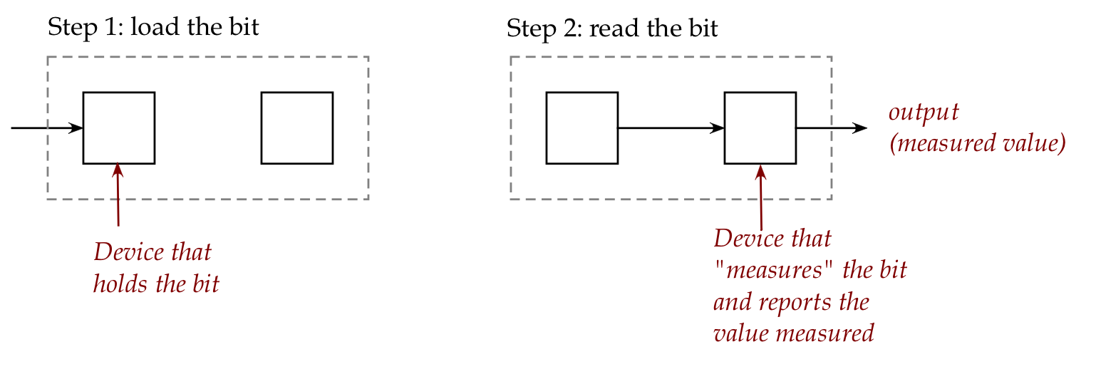
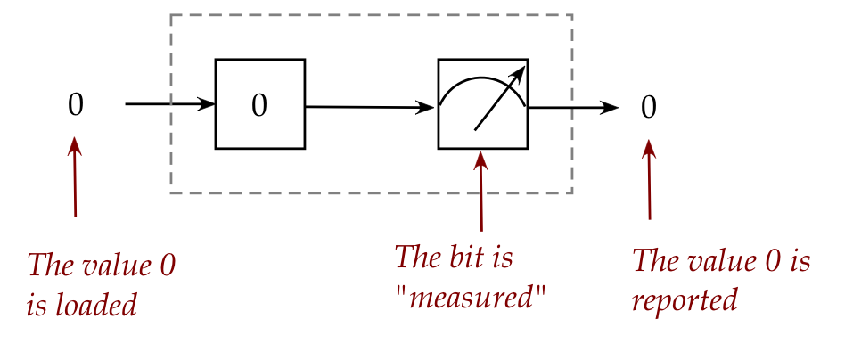
Let's start by examining the behavior of a classical bit:
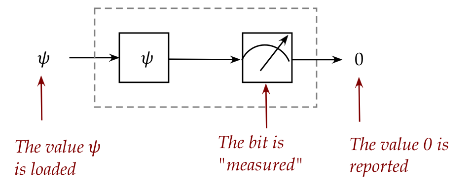
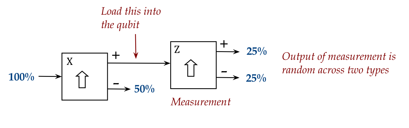
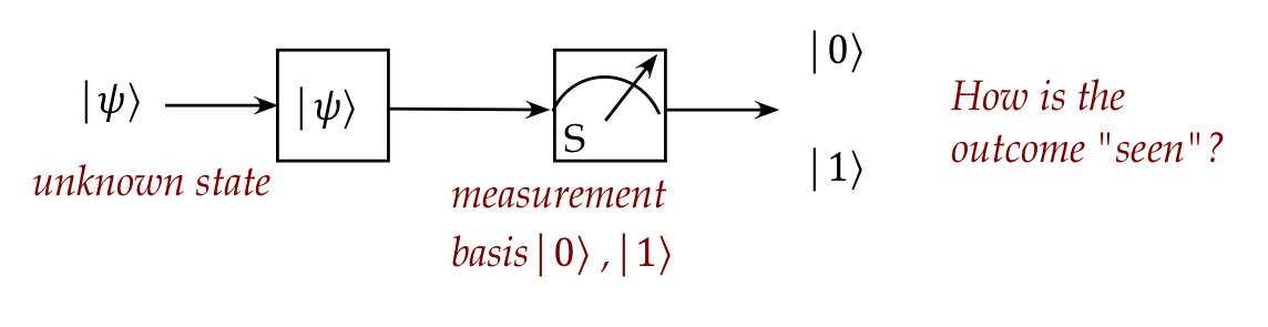
Let's now do the same experiment with a qubit:
- Qubit = Quantum bit
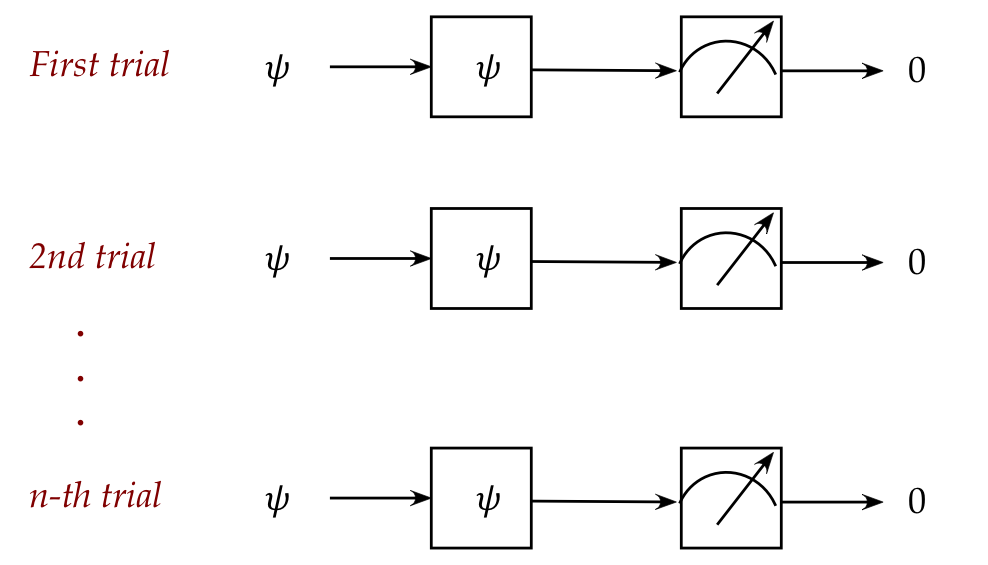
- Here's an example of some trials for a qubit:
Note:
- We now cannot assert a definitive value for the unknown value
\(\ksi\).
- Multiple repetitions do not yield exactly the same value.
- In fact, statistical analysis over many trials shows that
the pattern of output is completely random between
\(\kt{0}\) and \(\kt{1}\)
- The measuring device performs an "S" measurement.
(Whatever that means. We'll clarify later.)
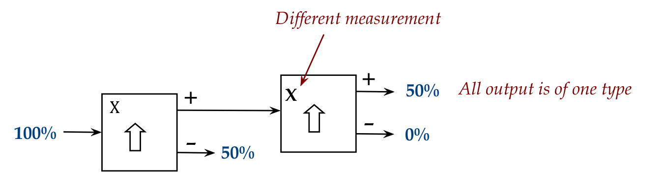
- What if we used a different measuring device?
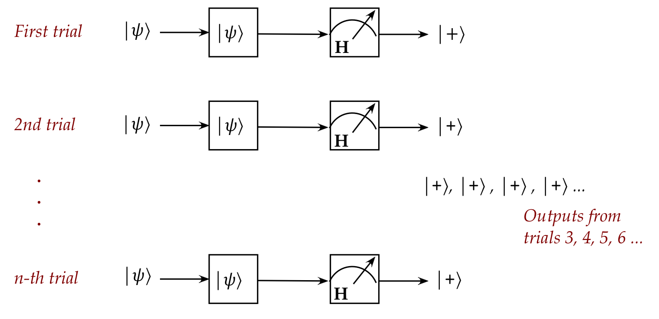
- Here, we have replaced an "S" device with an "H" measurement device.
- This time the output is entirely predictable!
- Does this remind you of anything from Module 1?
- In fact, a Stern-Gerlach apparatus is a qubit:
- There are many such two-level quantum systems that
can serve as qubit technology.
- The SG apparatus is not at all practical.
\(\rhd\)
Other technologies are much more practical and successful.
-
What's useful: the same theory works for all two-level systems (devices).
So, what exactly is a qubit?
- Answer: A qubit is a device that holds a unit-length 2D complex vector as
its value.
- Consider for example, the complex vector
$$
\ksi \eql \vectwo{\alpha}{\beta}
$$
Is \(\ksi\) a qubit value?
- Yes!
- And it's a qubit value for any (unit-vector-length) choice of the complex
numbers \(\alpha, \beta\).
- Example qubit values:
$$
\ksi \: = \: \vectwo{1}{0},
\;\;\;\;\;\;
\ksi \: = \: \vectwo{0}{1},
\;\;\;\;\;\;
\ksi \: = \: \vectwo{\isqt{1}}{\isqt{i}},
\;\;\;\;\;\;
$$
- Note that a qubit vector can be expressed in any desired
basis:
- Example: \(\ksi = (\alpha, \beta)\) in the standard basis:
$$
\ksi \eql \vectwo{\alpha}{\beta}
\eql \alpha \vectwo{1}{0} + \beta \vectwo{0}{1}
\eql \alpha \kt{0} + \beta \kt{1}
$$
- Example: \(\ksi = \kt{0}\) in the Hadamard basis:
$$
\kt{0} \eql \isqts{1} \kt{+} + \isqts{1} \kt{-}
$$
This is important, as we'll soon see.
- Terminology:
- The vector \(\ksi\) that we've called the qubit's
value is more often called the state of the qubit.
- \(\ksi\) is also called the quantum state vector,
and occasionally, the wavefunction.
- \(\ksi\) is also called a ket (we won't use this nomenclature).
- We can already see one implication:
- The set of possible values for a single qubit
is (uncountably) infinite.
$$
\ksi \eql \vectwo{\alpha}{\beta}
\mbx{\(\alpha, \beta\) are complex numbers}
$$
- Let's address the obvious question: do we impose
the set of qubit values and then build hardware to
support such qubits?
- No! This is what qubits are, and the theory follows
from their natural behavior.
- All two-level quantum systems are modeled by 2D complex vectors
\(\rhd\)
This might be unsettling, but this is how nature is.
- There's more that's perplexing, as we'll see.
- We still need to address:
- Where does the randomness come in?
- Why do we get different results with different types of
measurements?
- What does it have to do with complex vectors?
3.2
Nature's indeterminism and the puzzle of measurement
Let's start with the measuring device:
- Think of a qubit measuring device as a 2D orthonormal basis:
- Example 1: Thus, for example, the basis
$$\eqb{
\kt{0} & \eql & \vectwo{1}{0}\\
\kt{1} & \eql & \vectwo{0}{1}\\
}$$
is one measuring device.
- Example 2: The basis
$$\eqb{
\kt{+} & \eql & \vectwo{\isqt{1}}{\isqt{1}}\\
\kt{-} & \eql & \vectwo{\isqt{1}}{-\isqt{1}}\\
}$$
is another measuring device.
- In general, any orthonormal 2D basis
$$\eqb{
\kt{v} &\eql & a \kt{0} + b \kt{1} \\
\kt{v^\perp} &\eql & b^* \kt{0} - a^*\kt{1} \\
}$$
is a single qubit measuring device.
- Note: in 2D, \(\kt{v^\perp}\) is the unique (unit-length)
vector orthogonal to \( \kt{v} \).
- Now, any qubit state \(\ksi\) can be expressed in terms
of a measurement device's basis:
- For example, consider the basis \(\kt{0}, \kt{1}\), and
$$
\ksi \eql \vectwo{\alpha}{\beta}
$$
Then,
$$
\ksi \eql \alpha \kt{0} + \beta \kt{1}
$$
expresses \(\ksi\) in the \(\kt{0}, \kt{1}\) basis.
- Another example:
consider the basis \(\kt{+}, \kt{-}\), and the vector
\(\ksi = \kt{0}\):
$$
\ksi \eql \isqts{1} \kt{+} + \isqts{1} \kt{-}
$$
expresses \(\kt{0}\) in the \(\kt{+}, \kt{-}\) basis.
Now let's explain randomness and measurement outcome:
- The three aspects to a single measurement:
- Every measurement of a qubit value is associated with a
measurement basis.
\(\rhd\)
Example: the basis \(\kt{0}, \kt{1}\)
- A particular measurement outcome will be a random selection
from one of the basis vectors.
\(\rhd\)
Thus, either \(\kt{0}\) or \(\kt{1}\) for the \(\kt{0}, \kt{1}\) basis
- Which basis vector becomes the random outcome is based on these
probabilities:
- Express the qubit's state in the measurement basis.
\(\rhd\)
Example: \(\ksi = \inr{0}{\psi}\kt{0} + \inr{1}{\psi}\kt{1}\)
- This means each basis vector will have a coefficient in
the expression:
\(\rhd\)
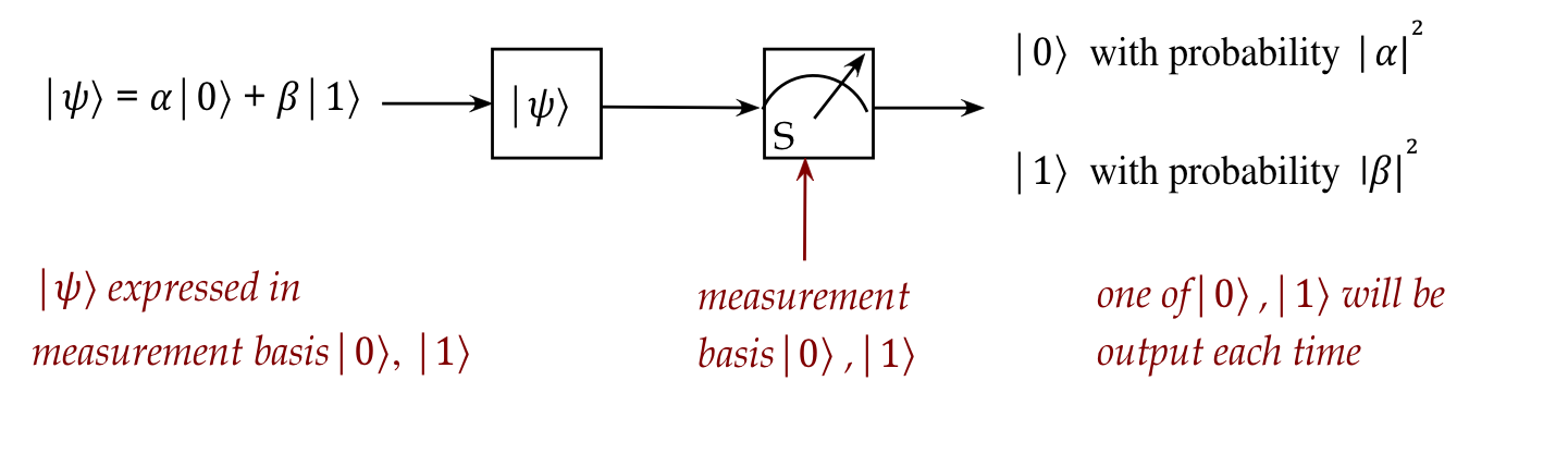
Example: \(\ksi = \alpha \kt{0} + \beta \kt{1}\)
- The probability of seeing a particular basis vector is
squared magnititude of the coefficient.
$$\eqb{
\mbox{Probability outcome is \(\kt{0}\)}
& \eql & \magsq{\alpha}\\
\mbox{Probability outcome is \(\kt{1}\)}
& \eql & \magsq{\beta}\\
}$$
- Note: squared-magnitude is a real number.
(Which, we'll make sure, is between \(0\) and \(1\) so that
it makes sense as a probability.)
- Example: Suppose we use the measurement basis \(\kt{0}, \kt{1}\) and
\(\ksi = \alpha \kt{0} + \beta \kt{1}\):
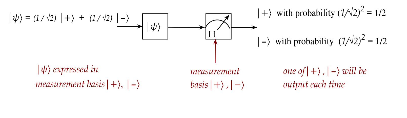
- Example: suppose we use the measurement basis \(\kt{+}, \kt{-}\) and
\(\ksi = \kt{0} = \isqt{1} \kt{+} + \isqt{1} \kt{-}\):
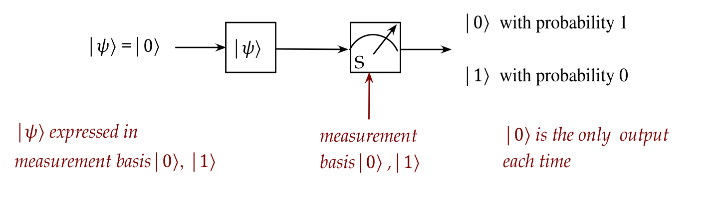
- Example: Suppose we use the measurement basis \(\kt{0},
\kt{1}\) and \(\psi = \kt{0}\)
- There is a more general way of describing measurement,
called projective measurement, that we'll see later.
In-Class Exercise 1:
Suppose the qubit state is \(\ksi = \kt{+}\) and the
measurement basis is:
\(\kt{w} = \frac{\sqrt{3}}{2} \kt{0} - \frac{1}{2} \kt{1}\),
and
\(\kt{w^\perp} = \frac{1}{2} \kt{0} + \frac{\sqrt{3}}{2} \kt{1}\).
What are the possible output vectors, and with what probabilities
do they occur? Start by expressing \(\kt{+}\) in
the \(\kt{w},\kt{w^\perp}\) basis by computing the
coefficients \(\inr{w}{+},\inr{w^\perp}{+}\).
Let's say a bit more about measurement:
- First, why is the output random?
- One might wonder: are measurement
devices deliberately constructed to perform random selection?
- And if so, why would anyone want to do that?
The answer to the first: No!
\(\rhd\)
This is just how nature is.
- The only time the measurement is not random is
when the outcome probability for one of the basis vectors
is \(1\).
\(\rhd\)
The case when the input is, in fact, that basis vector.
- In general, any measurement of any quantum state (in any quantum device)
is going to involve random output.
- That is, one cannot construct a measurement device
that avoids the randomness for all (even most) states.
- Why do we bother with measurement when the outcome is
uncertain? Why not just observe the qubit value?
- This is another unsettling issue: the only way to
know a qubit's state is to measure it.
- To summarize so far:
- To examine a qubit's state, one must measure.
- A measurement outcome is random, and is one of the
measurement-basis vectors.
Another piece of the puzzle:
Yet another piece of the puzzle:
- We have said that a state cannot be observed, only measured.
- How then do we know which measurement outcome state
occurred?
\(\rhd\)
Isn't that a form of observation?
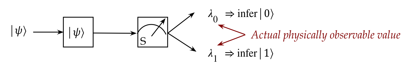
- A measurement is accompanied by a physical value that
can be observed, such as energy (frequency):
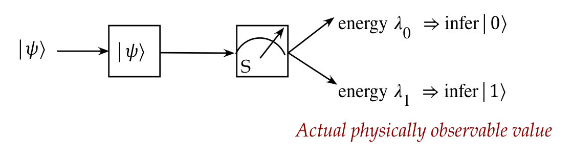
- Every unique outcome (a vector)
has a unique accompanying physical value (a number):
- If this sounds suspiciously like "different eigenvectors have
different eigenvalues"
\(\rhd\)
That's because it is the case!
- Actual measurement hardware detects the value of the
accompanying physical value or signal.
3.3
Stationary vs flying qubits
We will distinguish between two types of hardware configurations:
stationary and flying qubits.
Both are identical in terms of theory, and so we will (as do all
books) use only the latter because it's more convenient to draw.
Think of a flying qubit as an atom or photon in motion:
- Consider a flying qubit \(\ksi = \alpha\kt{0} + \beta \kt{1}\)
entering a standard-basis measuring device.
- Suppose measurement resulted in \(\kt{0}\).
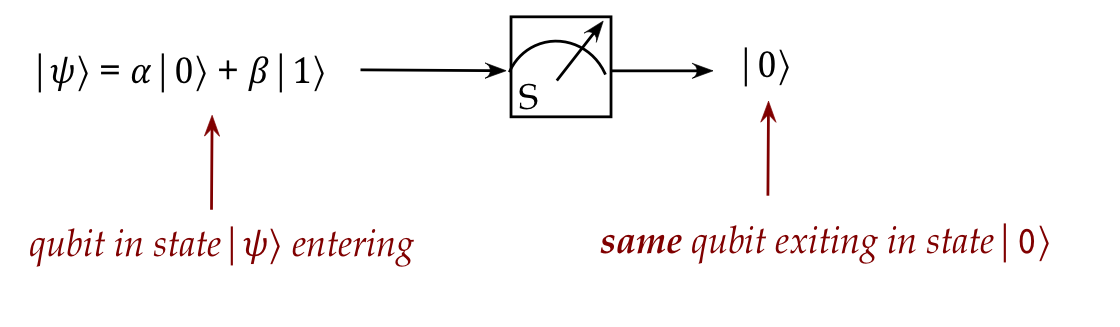
- A qubit enters from the left (in this picture) in the
\(\alpha\kt{0} + \beta \kt{1}\) state.
- After measurement, its new state happens to be \(\kt{0}\).
- That is, there's only one qubit in play here.
- The changed qubit can now be directed towards other devices,
perhaps to a measurement in another basis.
Think of a stationary
qubit as the state of an atom's outermost electron:
- For example, here are three qubits in three different states.
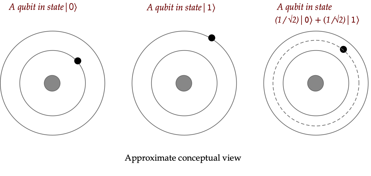
Here:
- Here, \(\kt{0}\) is typically the lowest energy or ground
state of the electron.
- \(\kt{1}\) is the excited state.
- The state \(\isqt{1}\kt{0} + \isqt{1}\kt{1}\) is depicted
above, on the right.
- Note:
- The above depiction is only an approximation for
a simplified high-level conceptual view.
- The actual location of an electron, and this "planetary
motion" view is actually not correct.
- It's more accurate to say the electron is in a quantum
state, to which various measurements can be made, including
location, momentum, and other properties.
- How does measurement work for a stationary qubit?
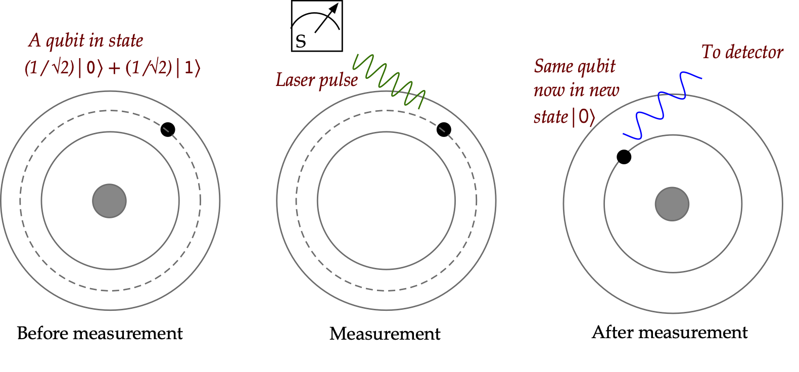
- Here, the measurement device is brought to the qubit
and activated.
- This changes the state of the qubit.
- There is some additional output that tells a detector
whether the post-measurement state is \(\kt{0}\) or \(\kt{1}\)
- The measurement device is then deactivated.
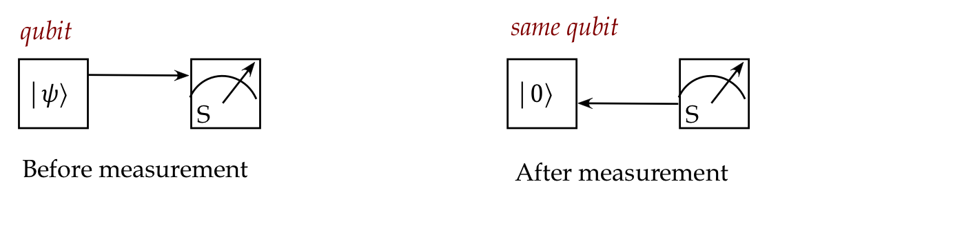
- Thus, using our conceptual boxes, we should really have
drawn something like this:
- The stationary kind of qubit is the more common
technology, and the one considered the most likely for
quantum computing.
The convention in drawing:
- The theory is exactly the same for both types of qubit configurations.
- The convention in books is to use the flying qubit diagram,
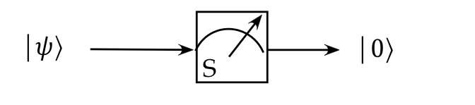
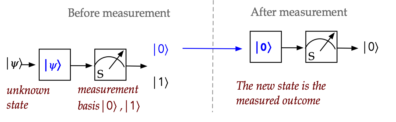
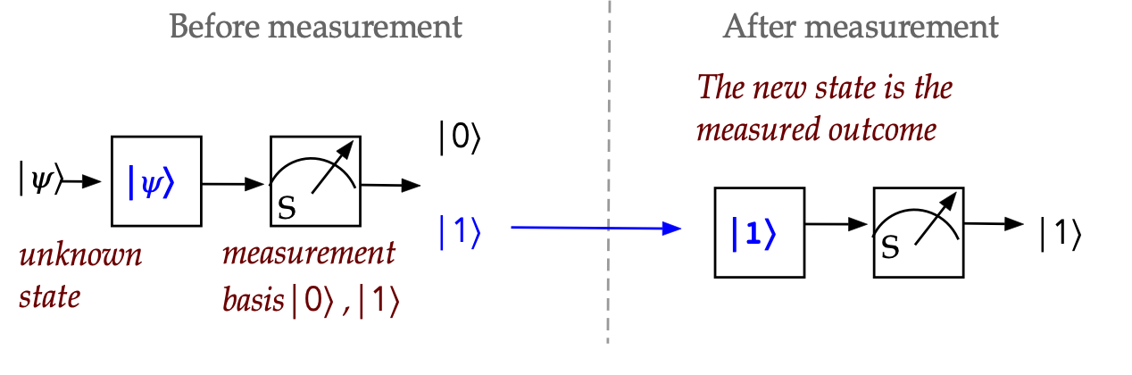
Measurement and initialization:
- Suppose we want to initalize a qubit into state \(\kt{0}\).
- At the start, suppose a qubit is in an unknown state \(\ksi\).
- We perform a measurement in the \(\kt{0}, \kt{1}\) basis.
- If this results in state \(\kt{0}\), we're done.
- We know that the state is now \(\kt{0}\).
- If not, we can change the state (next section) and apply
measurement again, repeating this whole process until a
measurement outcome is \(\kt{0}\).
3.4
What can you do with a qubit?
If all we could do is measure, we would not get far with quantum
computing.
Luckily, nature lets us modify a qubit's state without
measurement.
However, there's one limitation:
\(\rhd\)
The only modification allowed is a unitary operation.
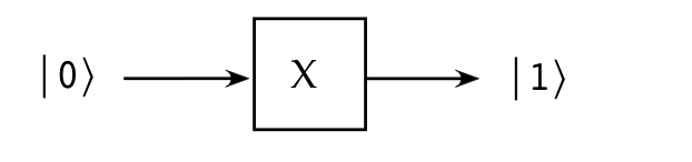
Let's look at an example:
- Consider the unitary operator
$$
\mat{0 & 1\\ 1 & 0}
$$
- Let's ask: what would we get if we applied this to a
qubit in state \(\kt{0}\)?
$$
X \kt{0}
\eql
\mat{0 & 1\\ 1 & 0}
\vectwo{1}{0}
\eql
\vectwo{0}{1}
\eql
\kt{1}
$$
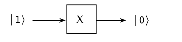
- We will diagram this as:
- Note that
$$
X \kt{1}
\eql
\mat{0 & 1\\ 1 & 0}
\vectwo{0}{1}
\eql
\vectwo{1}{0}
\eql
\kt{0}
$$
which we can depict as
- Observe that applying X twice results in
$$
X X \eql
\mat{0 & 1\\ 1 & 0}
\mat{0 & 1\\ 1 & 0}
\eql
\mat{1 & 0\\ 0 & 1}
$$
That is, the original state is returned.
In-Class Exercise 2:
What does the \(X\) gate do to the state
\(\ksi = \alpha\kt{0} + \beta\kt{1}\)?
Another example:
- Consider the Hadamard matrix
$$
H \eql
\mat{ \isqt{1} & \isqt{1}\\
\isqt{1} & -\isqt{1}}
$$
This is unitary as can be seen:
$$
H^\dagger H \eql
\mat{ \isqt{1} & \isqt{1}\\
\isqt{1} & -\isqt{1}}
\mat{ \isqt{1} & \isqt{1}\\
\isqt{1} & -\isqt{1}}
\eql I
$$
Thus, it can be used to modify a qubit's state.
- An aside:
- We've seen the H matrix in many roles.
- For example, it was a change-of-basis matrix.
- And because it's Hermitian, it served as an example then.
- The Hadamard matrix is one of the most important tools
in quantum computing.
- Now let's see what it does to \(\kt{0}, \kt{1}\):
$$\eqb{
H \kt{0} & \eql &
\mat{ \isqt{1} & \isqt{1}\\
\isqt{1} & -\isqt{1}}
\vectwo{1}{0}
\eql \vectwo{\isqt{1}}{\isqt{1}}
\eql \kt{+} \\
H \kt{1} & \eql &
\mat{ \isqt{1} & \isqt{1}\\
\isqt{1} & -\isqt{1}}
\vectwo{0}{1}
\eql \vectwo{\isqt{1}}{-\isqt{1}}
\eql \kt{-} \\
}$$
- Thus, the H operator
- transforms the state \(\kt{0}\) into the state \(\kt{+}\);
- transforms the state \(\kt{1}\) into the state \(\kt{-}\);
- What does it do to the general standard-basis vector
\(\ksi = \alpha\kt{0} + \beta\kt{1}\)?
$$
H \ksi
\eql
\smm{\frac{\alpha + \beta}{\sqrt{2}}} \kt{0}
+
\smm{\frac{\alpha - \beta}{\sqrt{2}}} \kt{1}
$$
In-Class Exercise 3:
Derive the above result that applies \(H\) to
\(\ksi = \alpha\kt{0} + \beta\kt{1}\).
Also show that \(H\ksi = \alpha\kt{+} + \beta\kt{-}\).
Now let's build our first circuit:
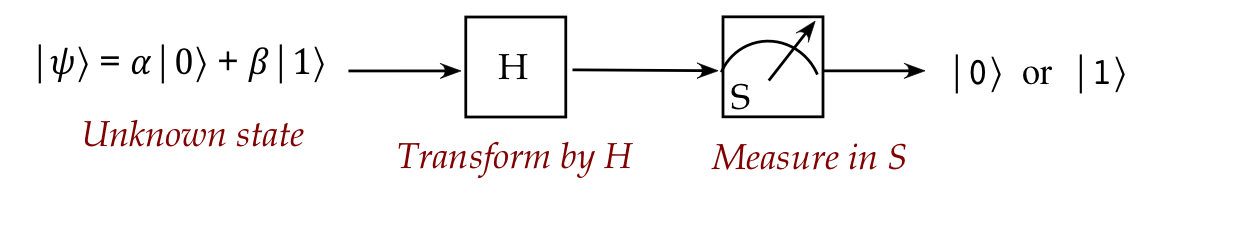
- We have an unknown state \(\ksi = \alpha\kt{0} + \beta\kt{1}\)
entering from the left.
- Applying the H transform results in
$$
H \ksi
\eql
\smm{\frac{\alpha + \beta}{\sqrt{2}}} \kt{0}
+
\smm{\frac{\alpha - \beta}{\sqrt{2}}} \kt{1}
$$
- Measuring in the standard basis yields
$$\eqb{
\kt{0} & \;\;\;\mbox{with probability } \;\;\;
\magsq{ \smm{\frac{\alpha + \beta}{\sqrt{2}}} }\\
\kt{1} & \;\;\;\mbox{with probability } \;\;\;
\magsq{ \smm{\frac{\alpha - \beta}{\sqrt{2}}} }\\
}$$
- Suppose we perform this experiment several times and
obtain \(\kt{0}\) much more often than \(\kt{0}\).
- This means the probability of obtaining \(\kt{0}\) is
much higher than the probability of getting \(\kt{0}\).
- That is,
$$\eqb{
\magsq{ \smm{\frac{\alpha + \beta}{\sqrt{2}}} }
& \; \approx \; & 1 \\
\magsq{ \smm{\frac{\alpha - \beta}{\sqrt{2}}} }
& \; \approx \; & 0 \\
}$$
- From which we conclude \(\alpha \approx \beta\).
- Thus, we've learned something about the unknown
state through a simple transformation.
- Of course, we could measure the unknown state repeatedly
and estimate in that manner too, but if we skew the probabilities
as above, we can arrive at the same result sooner.
Another example:
- Consider the strangely-named matrix
$$
\sqrt{X}
\eql
\mat{ \frac{1+i}{2} & \frac{1-i}{2}\\
\frac{1-i}{2} & \frac{1+i}{2}}
$$
- Is it unitary?
$$
\left( \sqrt{X} \right)^\dagger
\eql
\mat{ \frac{1-i}{2} & \frac{1+i}{2}\\
\frac{1+i}{2} & \frac{1-i}{2}}
$$
Then it's easy to calculate
$$
\left( \sqrt{X} \right)^\dagger \: \sqrt{X} \eql I
$$
- Observe that
$$
\sqrt{X} \: \sqrt{X}
\eql
\mat{ \frac{1+i}{2} & \frac{1-i}{2}\\
\frac{1-i}{2} & \frac{1+i}{2}}
\mat{ \frac{1+i}{2} & \frac{1-i}{2}\\
\frac{1-i}{2} & \frac{1+i}{2}}
\eql
\mat{0 & 1\\ 1 & 0}
\eql X
$$
Thus, the effect of applying \(\sqrt{X}\) twice is the
same as applying \(X\).
- While \(X\) has a natural classical analog, the NOT Boolean
gate, \(\sqrt{X}\) has no classical analog.
Some terminology:
- A unitary operator is called a quantum gate, or just
gate.
- Superposition:
- A vector such as \(\isqt{1} \kt{0} + \isqt{1}\kt{1}\) or
\(\alpha \kt{0} + \beta \kt{1}\) that is a linear combination
of basis vectors is sometimes called a superposition.
- About superpositions:
- Any superposition requires specifying the basis used
in the linear combination.
- A superposition is not a simultaneous occurence of
the basis vectors involved.
- It's just a vector that happens to be expressible as a
linear combination of basis vectors.
- Clearly, a particular vector can be a superposition in
one basis (e.g., \(\kt{+} = \isqt{1} \kt{0} + \isqt{1}\kt{1}\))
but not so in another basis (e.g, \(\kt{+}\) in the
\(\kt{+},\kt{-}\) basis).
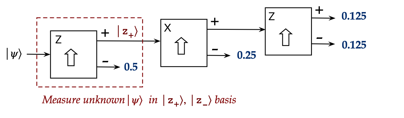
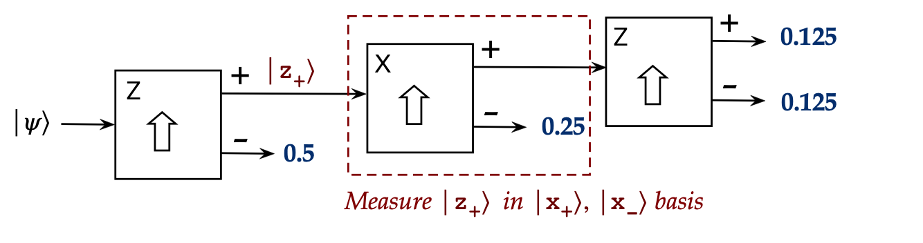
In-Class Exercise 4:
Consider the two circuits below, each given the same input.
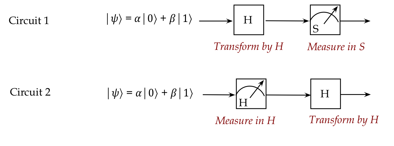
- Write down the possible states of the outputs.
- Calculate the probabilities associated with each output state.
3.5
The promise and challenge of quantum computing viewed through a qubit
What we've seen so far gives us a hint
of the promise and challenge in quantum computing.
First, the promise:
- Compared to a regular bit, a qubit can be in one of an infinite
number of states.
- A unitary operator can be applied to any qubit, not just
the two standard-basis states \(\kt{0}, \kt{1}\).
- It's natural to equate \(\kt{0}, \kt{1}\) with regular bits \(0\)
and \(1\).
- We will later see how regular logic circuits can be converted
to quantum equivalents, showing that a quantum circuit can do what
a logic circuit can do.
- But quantum states are many more!
- Consider the state
$$
\kt{+} \eql \isqts{1}\kt{0} + \isqts{1}\kt{1}
$$
This is a linear combination of the two states
\(\kt{0}, \kt{1}\):
- It is incorrect to think of this as a "mixture" of the
two states \(\kt{0}, \kt{1}\).
- \(\kt{+}\) is a state, period.
- It can be expressed as a linear combination of all kinds of
basis vectors.
- We will later see that it's possible to create
a 2-qubit state like
$$
\smm{\frac{1}{2}} \left(
\kt{00} + \kt{01} + \kt{10} + \kt{11}
\right)
$$
That is, a combination of all four 2-qubit basis states.
- We will see later that \(n\) qubits will have \(2^n\) basis states.
- Then, one can create a single state
that combines (through linear combination) all \(2^n\) basis states!
- This suggests that we can compute simultaneously with all
basis states
\(\rhd\)
In fact, this is often the starting point for many quantum algorithms.
- There is also a multi-qubit property
called entanglement that's both mystifying and powerful,
which we will exploit.
- In combination, all these properties will show that quantum
computers can:
- perform some computations that no classical computer is known
to perform in reasonable time;
- perform some computations provably faster than a classical
computer (so-called quantum supremacy).
But ... there are many challenges in exploiting this power:
- Measurement has probabilistic outcomes:
- This may mean repeating a computation until one has a result
with high probability.
- Measurement destroys quantum state, replacing it with one of
the measurement basis vectors:
- This means one typically uses measurement only after a
sequence of unitary operations.
- Although, as we will see later, unitary operations can
simulate any classical logic circuit, there are added gates needed,
which impacts efficiency.
- These are just the theoretical "in principle" challenges.
- The hardware challenges are even more significant:
- Quantum states don't last long and thus unitary operations
must be performed quickly.
- The slightest bit of noise (decoherence)
can derail any computation:
- Random changes in environment (ion movement)
- Unintended entanglement with other qubits or environment
- Imprecision in control (clocks, lasers etc)
- It's difficult to work with multiple qubits.
- Currently, hardware needed for cooling is expensive.
- Nonetheless, as of 2024, some vendors claim
to have demonstrated
computations on 48 error-corrected qubits.
- Note: a logical qubit is an error-corrected
qubit that is itself a composite of regular hardware qubits.
3.6
Revisiting the light polarization experiment
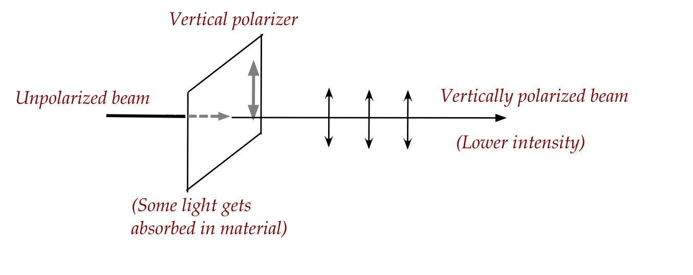
Recall the phenomenon of polarization:
The same experiment with single photons:
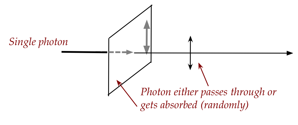
Now consider the first of two experiments:
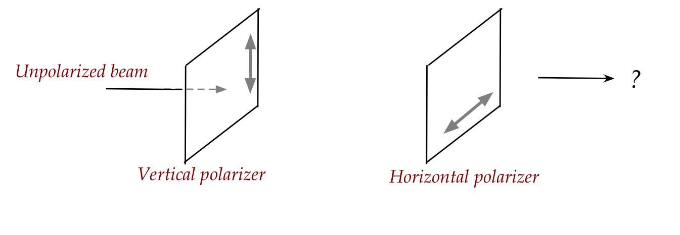
In this scenario:
- Careful experimentation shows that:
no light emerges from the second polarizer.
- The same result obtains when sending a single photon at a time.
- For single photons:
- The photon either gets absorbed or passes through the first polarizer.
- A photon that passes the first is always absorbed by the second polarizer.
Now consider the second scenario:
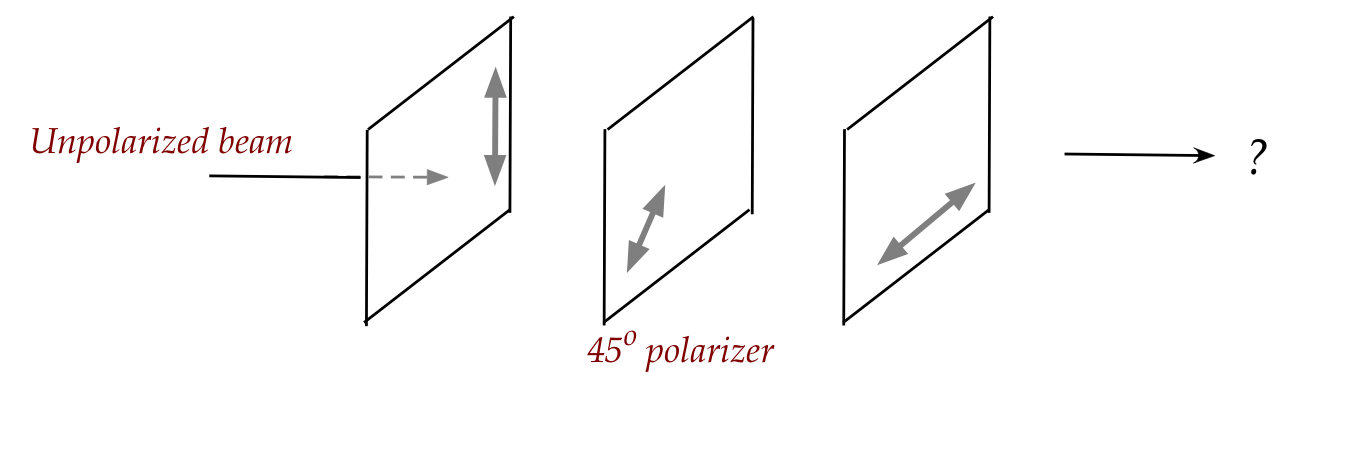
In this case:
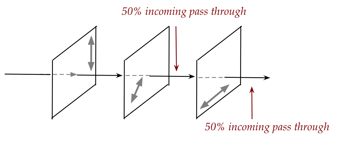
- Photons are randomly either absorbed or pass through the first polarizer.
- Here's the key observation:
50% of the photons that reach the middle polarizer pass through.
- Of the photons that reach the third, 50% pass through.
While a classical explanation can be constructed for beams
of light, no classical reasoning explains the single-photon experiments.
Now let's provide a quantum explanation:
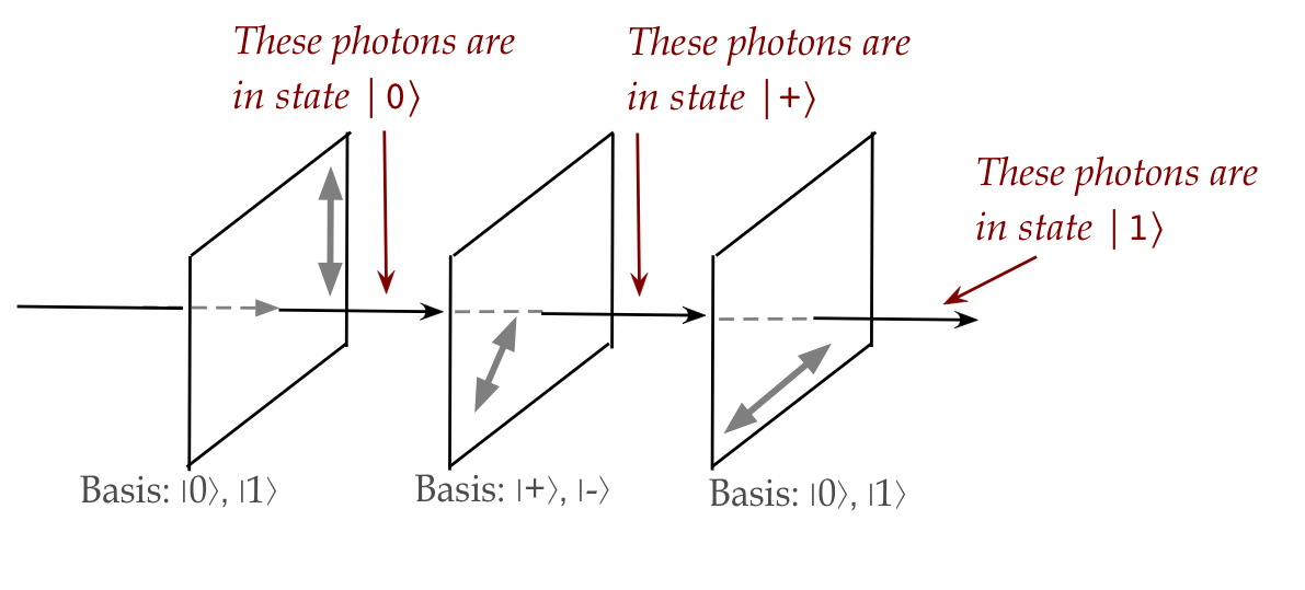
- Each polarizer is a measuring device.
- The bases used by the first and third are:
- The first polarizer uses:
$$\eqb{
\kt{0} & \eql & \mbox{pass through, vertically polarized} \\
\kt{1} & \eql & \mbox{absorb} \\
}$$
- The third polarizer uses:
$$\eqb{
\kt{1} & \eql & \mbox{pass through, horizontally polarized} \\
\kt{0} & \eql & \mbox{absorb} \\
}$$
- The middle one is more interesting:
$$\eqb{
\kt{+} & \eql & \isqts{1} \kt{0} + \isqts{1} \kt{1}
& \eql & \mbox{pass through, polarized at \(45^\circ\)} \\
\kt{-} & \eql & \isqts{1} \kt{0} - \isqts{1} \kt{1}
& \eql & \mbox{absorb} \\
}$$
- Now consider a photon of unknown polarization arriving
at the first polarizer:
- The photon's polarization can be written in terms of the
measuring device's \(\kt{0}, \kt{1}\) basis.
- Since it can be anything, we model the photon's polarization
as \(\alpha \kt{0} + \beta \kt{1}\).
- The probability that it passes through, therefore, is
$$
\magsq{\alpha} \eql \mbox{probability of passing through}
$$
- After passing through, it will be in the \(\kt{0}\) state.
\(\rhd\)
Vertically polarized.
- Now let's look at a photon arriving at the middle polarizer:
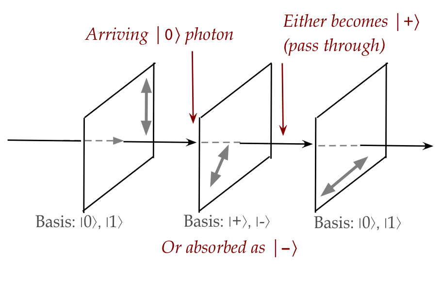
- The photon arrives in the state \(\kt{0}\).
- The middle polarizer is a measuring device with basis
vectors
$$\eqb{
\kt{+} & \eql & \isqts{1} \kt{0} + \isqts{1} \kt{1}
& \eql & \mbox{pass through, polarized at \(45^\circ\)} \\
\kt{-} & \eql & \isqts{1} \kt{0} - \isqts{1} \kt{1}
& \eql & \mbox{absorb} \\
}$$
- We now express the incoming photon in the measuring device's basis:
$$
\kt{0} \eql \isqts{1} \kt{+} + \isqts{1} \kt{-}
$$
- The probability of passing through is therefore
$$
\mbox{Pr[pass through]} \eql
\magsq{ \isqt{1} } \eql \frac{1}{2}
$$
This is what gives us the 50% pass through rate.
- The photon that passes through now has the state \(\kt{+}\).
- Finally, let's look at the last polarizer:
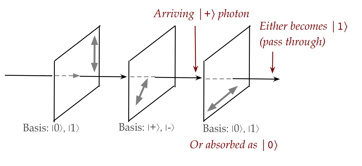
- The arriving photon is in the \(\kt{+}\) state.
- The basis of the polarizer is:
$$\eqb{
\kt{1} & \eql & \mbox{pass through, horizontally polarized} \\
\kt{0} & \eql & \mbox{absorb} \\
}$$
- Express the photon's state in the measurement basis:
$$
\kt{+} \eql \isqts{1} \kt{0} + \isqts{1} \kt{1}
$$
- Thus, the probability that it passes through is:
$$
\mbox{Pr[pass through]} \eql
\magsq{ \isqt{1} } \eql \frac{1}{2}
$$
- Note:
- Photons can have their state changed by unitary operations.
- Thus, photons can be made into flying qubits for computation.
- This will result in our first real application - in the next section.
In-Class Exercise 5:
Consider the following set up:
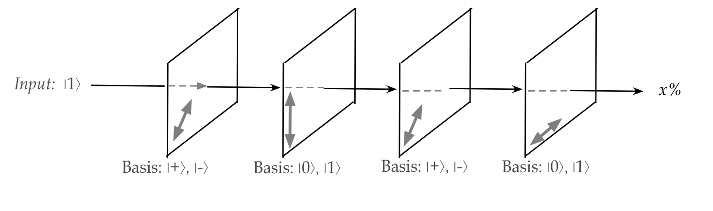
What percentage of \(\kt{1}\) photons arriving on the left
reach the output? Work through your probability calculations as
shown above.
3.7
An application of single qubits: quantum key distribution
The goal of QKD (Quantum Key Distribution) is to enable
unconditionally secure communication between two parties,
typically called Alice and Bob.
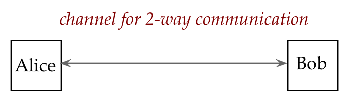
Let's start by exploring some terms and the context:
- We use the abstract term channel to represent any
medium of communication between Alice and Bob:
- Example: mission control (Alice) to satellite (Bob) via
radio waves (channel).
- Example: Headquarters (Alice) to regional bank office (Bob)
over the internet (channel).
- Alice and Bob can use a one-time pad, which is
unconditionally secure:
- They meet or securely-courier a shared
book of random integers.
\(\rhd\)
This is not done using the channel but up front and securely.
- Subsequent text messages are encoded using these numbers,
with a fresh page used for each message.
- Because the number patterns are never re-used, an adversary
cannot gain any information statistically.
- And there are (incorrect) number patterns that will decode to
valid text, making it impossible to judge whether a lucky guess is correct.
- The big downside of course is the inconvenience of sharing
the one-time pads, and keeping them secure.
- Alternatively, Alice and Bob can use a short-term secret key,
which is a sequence of random integers, and re-use that key
for near-term messages:
- These keys can be created afresh periodically.
- The problem of sharing such keys is called key distribution.
- To share such keys without meeting, Alice and Bob use
public-key cryptography.
- However, public-key cryptography relies on the hypothesis
that the underlying mathematical problem cannot be easily solved:
- Factoring (large) integers, as in the RSA public-key system.
- The discrete log problem for elliptic-curve cryptography.
- As we will see in this course, a quantum computer can efficiently
solve the former directly using Shor's algorithm, which can also
used indirectly to solve the latter.
The adversary:
- In any security solution, one must model the adversary
\(\rhd\)
Often called the threat model.
- The primary attack we'll consider is "tapping into the line"
- Here, the attacker can receive the photons Alice sends.
- The attacker can either try to decipher, or both decipher
and send photons along to Bob in order to evade detection.
- There are other, more sophisticated attacks we'll consider
in a later module.
Main ideas in quantum key distribution using the BB84 Protocol:
- BB84: Bennett and Brassard in 1984 (first such paper).
- BB84 aims to get a bit pattern securely from Alice to Bob.
- The protocol depends on the ability to send single qubits
in particular states:
- In today's technology, the only practical flying qubit is a photon.
- Thus, the protocol relies on reliable single-photon transmission.
\(\rhd\)
Which is hard to do, but has been demonstrated over distances
beyond 100km.
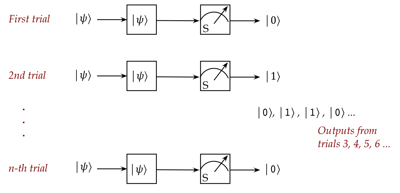
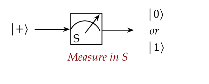
- The protocol also relies on being able to produce truly
random bits:
- This is easy with quantum technology.
- For example, one simply feeds \(\kt{+}\) qubits to a
standard-basis measurement:
- The protocol uses two channels:
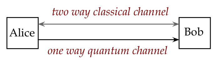
- The quantum channel transports qubits.
- The classical channel (which may have weaker security)
is used for messages.
Let's examine the steps in BB84:
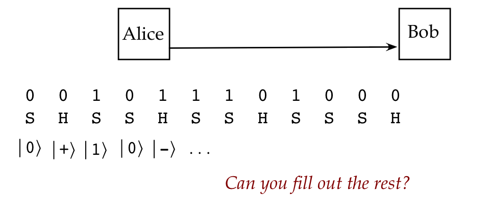
- Step 1 (Alice):
Alice creates a random bit string on her side, for
example
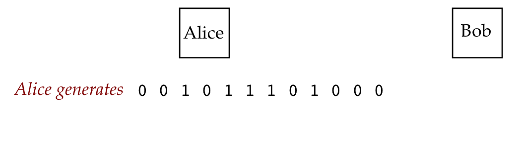
We'll call these the (classical) initial potential key bits.
- Step 2 (Alice):
Alice creates a random string using the letters "S" and "H",
lining them up with the key bit pattern.
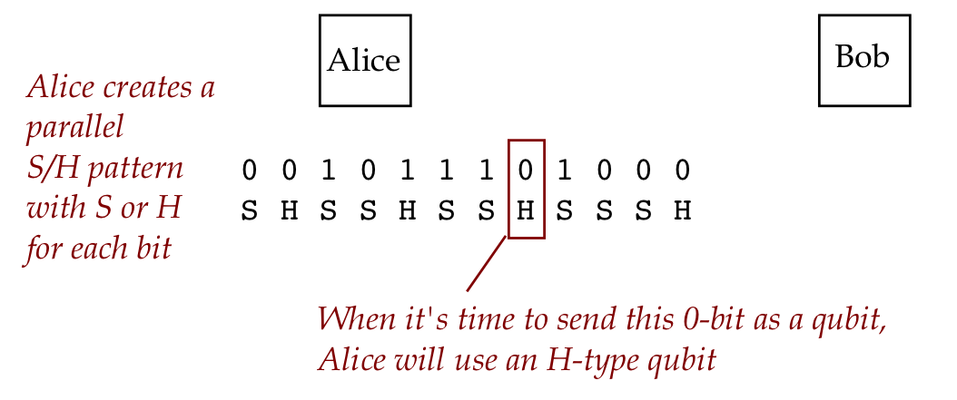
- If a key bit is aligned with "S", she uses an S-type
qubit for that bit.
- Otherwise, an "H" type qubit.
- Step 3 (Bob):
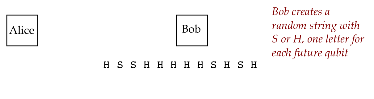
Bob's random string using the letters "S" and "H",
will be used later in lining them up with the qubits that
Alice will send.
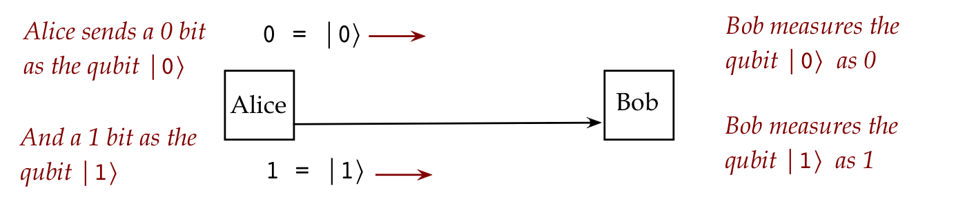
- Step 4 (Alice):
Alice sends her qubits one by one, but using qubit values
dictated by the S-H string:
- If a particular qubit has been designated an S-type qubit,
then
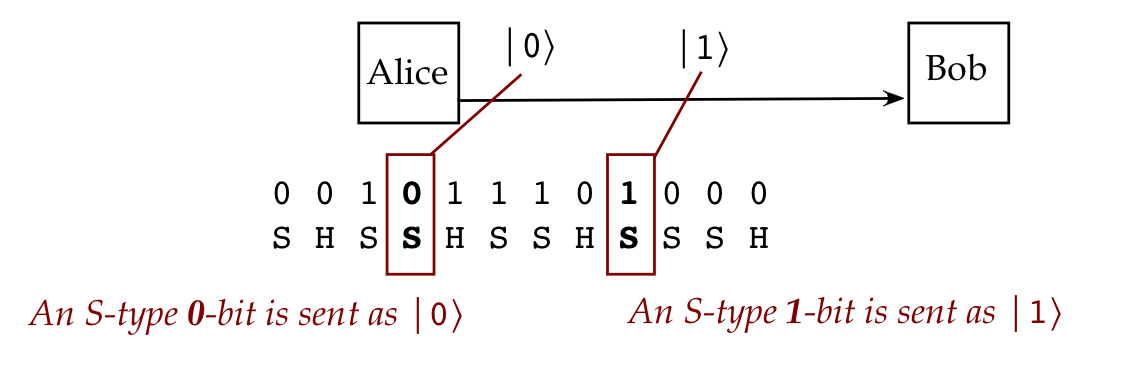
- \(0\) key bit \(\Rightarrow\) send \(\kt{0}\)
- \(1\) key bit \(\Rightarrow\) send \(\kt{1}\)
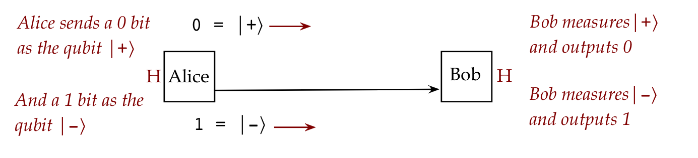
- If a particular qubit has been designated an H-type qubit,
then
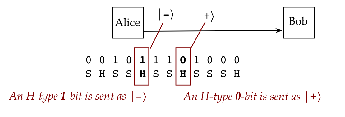
- \(0\) key bit \(\Rightarrow\) send \(\kt{+}\)
- \(1\) key bit \(\Rightarrow\) send \(\kt{-}\)
In this manner, all the key bits get sent as S or H qubits:
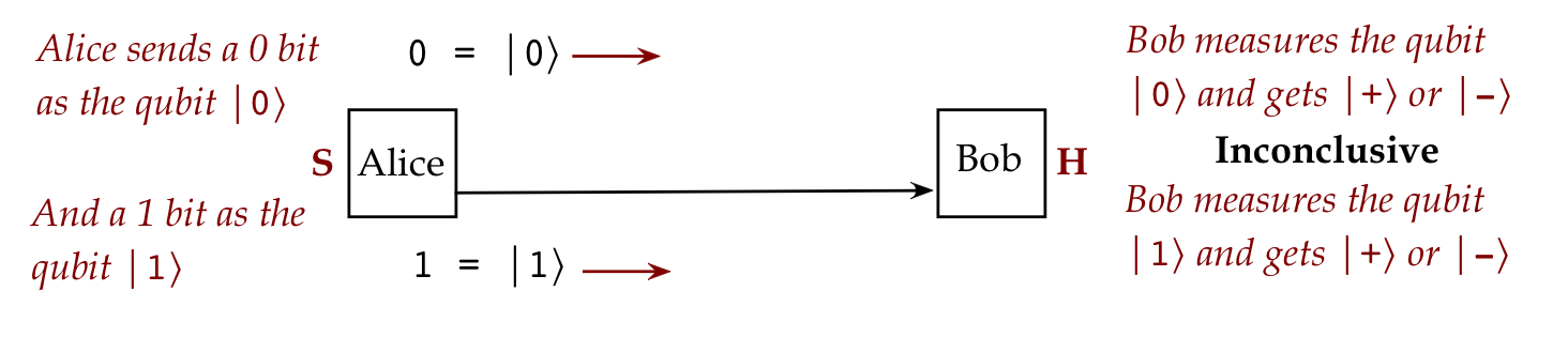
- Step 5: (Bob)
Bob measures these qubits as they arrive, using for each arriving qubit
one of two bases, as dictated by his "S-H" string.
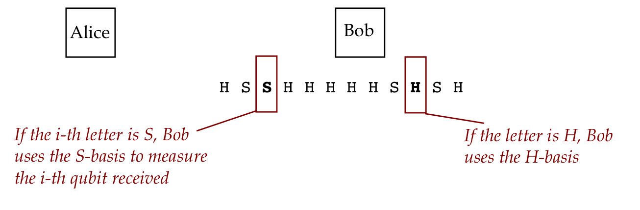
- If the i-th letter is S, he uses the standard-basis,
\(\kt{0}, \kt{1}\),
to measure the i-th qubit.
- If he obtains \(\kt{0}\), he infers \(0\) as the key bit.
- Otherwise \(1\).
- Otherwise he uses the Hadamard basis,
\(\kt{+}, \kt{-}\),
- If he obtains \(\kt{+}\), he infers \(0\) as the key bit.
- Otherwise \(1\).
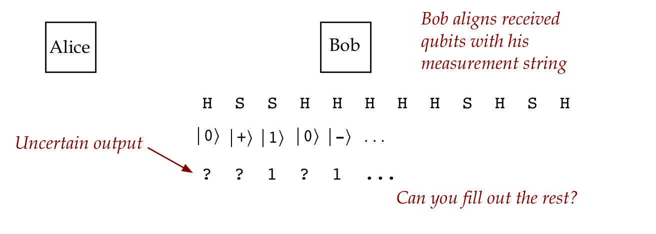
So, at the end of receiving all the qubits, Bob will have
a key bit-string aligned with his S-H string:
- Step 6: (Alice and Bob)
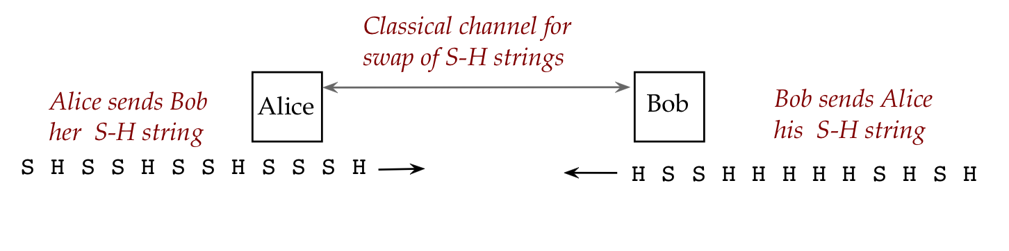
They use the classical channel to send each other their S-H strings.
- Step 7: (Alice and Bob)
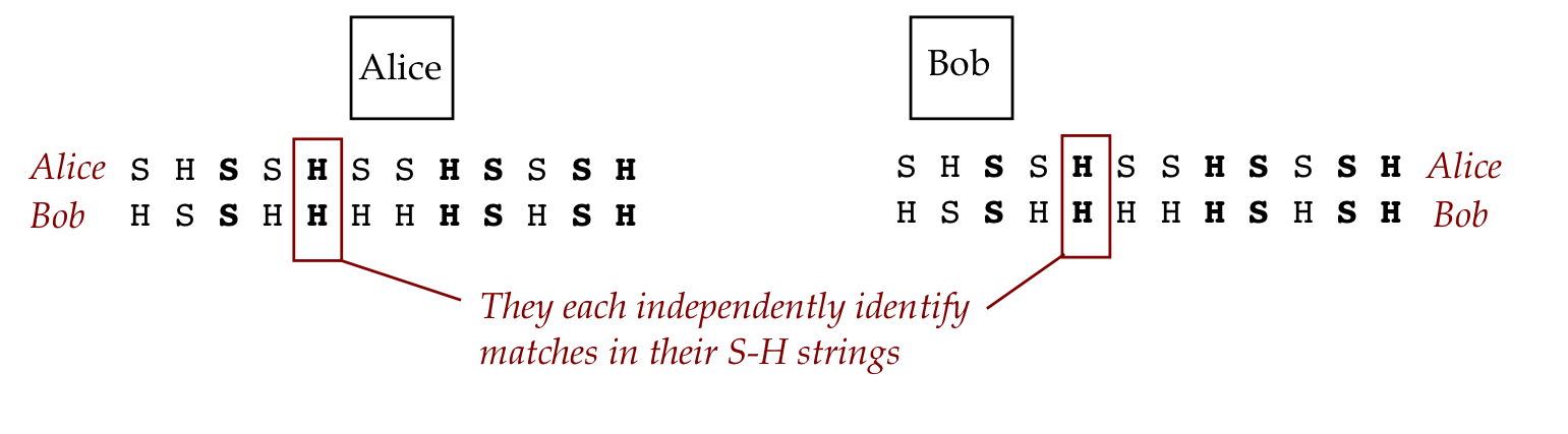
They each identify the positions in their S-H strings where
their letters match.
- Step 8: (Alice and Bob)
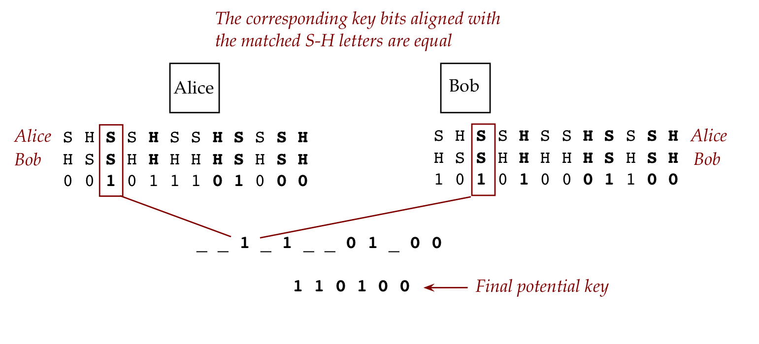
The bits in the positions where S-H aligned are identical
- We'll call these the final potential key bits.
(The final actual key bits will need one more step - see below.)
Note: the other bits may differ.
Let's first examine correctness, assuming no attacker (Eve) is present.
In-Class Exercise 6:
- What would go wrong if the S-H strings were exchanged before
Bob performs qubit measurements?
- Write out the details of Case 2(B) above, explaining the
details of measurement and probabilities.
Let's now focus on Eve:
- Eve the eavesdropper, that is.
- What can Eve do?
- Eve can try to copy (some or all of)
the qubits by tapping the optical fiber.
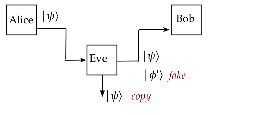
- Eve can capture Alice's qubits and send fake qubits to Bob.
- Eve can pose as Alice to Bob (impersonate).
Let's look at these one by one.
- We will later prove a simple but dramatic result:
it is physically impossible, in general, to copy qubits exactly
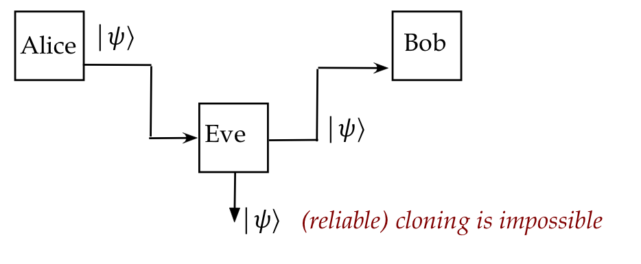
- This is called the No-Cloning Theorem.
- There are some caveats, but in general, a clean accurate copy
of a qubit can't be made without affecting the original.
- If Eve tries to intercept a few qubits, she'll have to
guess which basis to use in measurement.
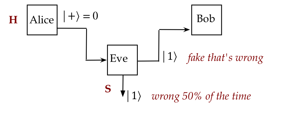
- Which means she'll be wrong 50% of the time (with random guessing).
- These qubits will change state because of measurement
- If she sends the changed qubits to Bob, then Alice and Bob
can detect this (as we'll show below).
- What happens if Eve impersonates Alice?
- BB84 does not solve this problem.
- The assumption is that the Alice and Bob can somehow authenticate
each other through the classical channel.
An improvement: detecting Eve
- Think of the agreed bits as the "good bits" (final potential
key bits)
- Alice and Bob, through the classical channel, share 50%
of their "good bits".
\(\rhd\)
This means the openly shared bits can't be used for the
secret key.
- If Eve intercepted qubits and sent fake ones, then 50%
of these supposedly good bits will differ between Alice and Bob.
\(\rhd\)
Eve will be caught.
- The remaining unshared good bits becomes the actual secret
key to be used for future encryption.
3.8
Phase equivalence in vectors
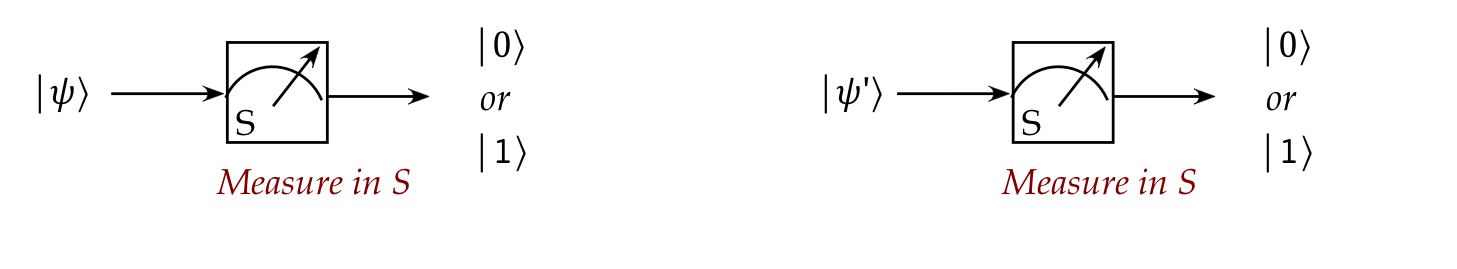
Consider these two vectors:
$$\eqb{
\ksi & \eql &
\smm{\frac{\sqrt{2}}{\sqrt{3}}} \kt{0} + \smm{\frac{1}{\sqrt{3}}} \kt{1}
& \eql &
\vectwo{ \frac{\sqrt{2}}{\sqrt{3}} }{ \frac{1}{\sqrt{3}} } \\
\kt{\psi^\prime} & \eql &
\smm{\frac{ 2-\sqrt{2} i}{3}} \: \kt{0}
+ \smm{\frac{\sqrt{2} - i}{3}} \: \kt{1}
& \eql &
\vectwo{ \frac{ 2-\sqrt{2} i}{3} }{ \frac{\sqrt{2} - i}{3} } \\
}$$
- Clearly, \(\ksi\) and \(\kt{\psi^\prime}\) are different
vectors because there's no simplification of the components
of \(\kt{\psi^\prime}\) that will result in \(\ksi\).
- Now consider the probability of obtaining \(\kt{0}\)
when each vector above is measured by in the S-basis (standard
basis):
- When the input vector is
$$
\ksi \eql
\smm{\frac{\sqrt{2}}{\sqrt{3}}} \kt{0} + \smm{\frac{1}{\sqrt{3}}} \kt{1}
$$
the probability of obtaining \(\kt{0}\) is:
$$
\mbox{Pr[\(\kt{0}\)]} \eql
\magsq{ \smm{\frac{\sqrt{2}}{\sqrt{3}}} }
\eql \smm{\frac{2}{3}}
$$
- With
$$
\kt{\psi^\prime} \eql
\smm{\frac{ 2-\sqrt{2} i}{3}} \: \kt{0}
+ \smm{\frac{\sqrt{2} - i}{3}} \: \kt{1}
$$
we get
$$
\mbox{Pr[\(\kt{0}\)]} \eql
\magsq{ \smm{\frac{ 2-\sqrt{2} i}{3}} }
\eql \smm{\frac{2}{3}}
$$
Both give the same results.
- Thus, experimentally, it is impossible to distinguish them
with the S-basis measurement.
- Now suppose we define the number
$$
a \eql \smm{\frac{2}{\sqrt{6}}} - i \smm{\frac{\sqrt{2}}{\sqrt{6}}}
$$
- The exercise below shows that
$$
\magsq{a} \eql 1
$$
and
$$
\kt{\psi^\prime} \eql a \ksi
$$
- Thus, we can write
$$\eqb{
\kt{\psi^\prime} & \eql & a \ksi \\
& \eql &
a
\parenl{
\smm{\frac{\sqrt{2}}{\sqrt{3}}} \kt{0} + \smm{\frac{1}{\sqrt{3}}} \kt{1} }\\
& \eql &
\smm{\frac{a \sqrt{2}}{\sqrt{3}}} \kt{0} + \smm{\frac{a}{\sqrt{3}}} \kt{0}
}$$
where the probability of obtaining \(\kt{0}\) in S-basis is
$$
\mbox{Pr[\(\kt{0}\)]}
\eql
\magsq{ \frac{a \sqrt{2}}{\sqrt{3}} }
\eql
\magsq{a} \magsq{ \frac{\sqrt{2}}{\sqrt{3}} }
\eql
\magsq{ \frac{\sqrt{2}}{\sqrt{3}} }
\eql
\frac{2}{3}
$$
- Here, multiplication by a unit-magnitude constant \(a\)
- changed the vector from \(\ksi\) to \(\kt{\psi^\prime}\);
- but did not affect the measurement probabilities.
- To clarify further, let's use
$$
\ksi \eql \alpha \kt{0} + \beta \kt{1}
$$
and
$$
\kt{\psi^\prime} \eql a \ksi
\eql
a \alpha \kt{0} + a \beta \kt{1}
$$
Then, \(\kt{\psi^\prime}\)
$$
\mbox{Pr[\(\kt{0}\)]}
\eql
\magsq{a \alpha}
\eql
\magsq{a} \magsq{\alpha}
\eql
\magsq{\alpha}
$$
which is the same probability when using \(\ksi\).
- Thus, for any complex number \(a\) such that
\(\magsq{a}=1\), the two vectors
\(\ksi\) and \(a\kt{\psi}\) are indistinguishable
with regard to S-basis measurements.
- This will be true for any measurement basis.
(See exercise below.)
- Thus, no experiment can reveal a measurable
difference between \(\ksi\) and \(\kt{\psi^\prime}\).
- These two vectors are considered to represent the
same quantum state and are called globally
phase-equivalent vectors.
In-Class Exercise 7:
Show that with \(a, \ksi\) and \(\kt{\psi^\prime}\) defined above,
- \(\magsq{a} \eql 1\)
- \(\kt{\psi^\prime} \eql a \ksi\)
Then, show that \(\ksi\) and \(a\ksi\) are indistinguishable
no matter what basis is used, as long as \(\magsq{a}=1\).
(Hint: express the standard-basis vectors in terms
of an arbitrary basis.)
This is an important point, so let's look at two more
examples, one with polar representation (later):
- Suppose
$$\eqb{
\kt{\phi} & \eql & \kt{0} \\
\kt{\phi^\prime} & \eql & i\kt{0} \\
}$$
- Here, \(a=i\) where \(|a|^2 = |i|^2 = 1\).
- Are these different states if measured in the \(\kt{+},\kt{-}\) basis?
- Express each in the measurement basis:
$$\eqb{
\kt{\phi} & \eql & \kt{0}
& \eql & \isqts{1} \kt{+} \: + \: \isqts{1} \kt{-}\\
\kt{\phi^\prime} & \eql & i\kt{0}
& \eql & \isqts{i} \kt{+} \: + \: \isqts{i} \kt{-}\\
}$$
- Then, when measuring \(\kt{\phi}=\kt{0}\)
$$
\prob{\mbox{Observe }\kt{+}} \eql \magsq{\isqt{1}} \eql \frac{1}{2}
$$
- And when measuring \(\kt{\phi^\prime}=i\kt{0}\),
$$
\prob{\mbox{Observe }\kt{+}} \eql \magsq{\isqt{i}}
\eql \frac{\magsq{i}}{\magsq{\sqrt{2}}}
\eql \frac{1}{2}
$$
- Thus, \(\kt{\phi}\) and \(\kt{\phi^\prime}\) are
indistinguishable through this measurement.
There is another, commonly used way of looking at
phase-equivalence, with the polar form:
- We know that any complex number \(a\) can be written as
$$
a \eql r e^{i\theta}
$$
When \(a\) has magnitude \(1\), then \(r=1\) and thus
$$
a \eql e^{i\theta}
$$
- Now consider any vector \(\ksi\) expressed in any basis
\(\kt{v}, \kt{v^\perp}\):
$$
\ksi \eql \alpha \kt{v} + \beta \kt{v^\perp}
$$
and let
$$
\kt{\psi^\prime} \eql a \ksi \eql e^{i\theta} \ksi
$$
- Then
$$
\kt{\psi^\prime} \eql
e^{i\theta} \alpha \kt{v} + e^{i\theta} \beta \kt{v^\perp}
$$
- Now when measured in the new \(\kt{v}, \kt{v^\perp}\) basis,
the probability of obtaining \(\kt{v}\)
$$
\mbox{Pr[\(\kt{v}\)]}
\eql
\magsq{ e^{i\theta} \alpha}
\eql
\magsq{ e^{i\theta}} \magsq{\alpha}
\eql
\magsq{\alpha}
$$
Thus, no measurement can distinguish the two vectors: both
represent the same quantum state.
- This is an important point so let's state it again in
a different way:
- No measurement (using any basis) can distinguish
between \(\ksi\) and \(e^{i\theta} \ksi\)
- Thus, even though \(\ksi\) and \(e^{i\theta} \ksi\)
are mathematically different vectors, they
represent the same physical state, the same quantum state.
- Terminology: \(\ksi\) and \(e^{i\theta} \ksi\)
are globally phase-equivalent.
- \(\ksi\) and \(e^{i\theta} \ksi\) have different
global phase.
- An aside: let's remember both ways of calculating
\(\magsq{ e^{i\theta}}\):
- The direct way:
$$
\magsq{ e^{i\theta}} \eql \left( e^{i\theta} \right)^* e^{i\theta}
\eql e^{-i\theta} e^{i\theta} \eql e^0 \eql 1
$$
- Or using Euler + trig:
$$
e^{i\theta} \eql \cos\theta + i\sin\theta
$$
and so
$$
\magsq{ e^{i\theta}} \eql \cos^2\theta + \sin^2\theta \eql 1
$$
Now let's look at the concept of relative phase:
- Consider two vectors we're already familiar with:
$$\eqb{
\kt{+} & \eql & \isqts{1} \kt{0} + \isqts{1} \kt{1} \\
\kt{-} & \eql & \isqts{1} \kt{0} - \isqts{1} \kt{1} \\
}$$
- At first glance, it may seem that the probability
of obtaining \(\kt{0}\) is the same for both vectors and
they should therefore be considered indistinguishable:
- Suppose \(\ksi\) is either \(\kt{+}\) or \(\kt{-}\)
but we don't know.
- Suppose we measure replicates of \(\ksi\) in S-basis
and obtain an estimate of \(\mbox{Pr}[\kt{0}]\).
- We won't be able to guess whether \(\ksi\) is \(\kt{+}\) or \(\kt{-}\).
- However, if we switch measurement to the H-basis,
that is the \(\kt{+}, \kt{-}\) basis, they are distinguishable:
- If a measurement in H-basis produces \(\kt{+}\) as outcome,
we are certain that \(\ksi = \kt{+}\).
- Thus, even though
$$
\kt{-} \eql \isqts{1} \kt{0} + e^{i\pi} \isqts{1} \kt{1} \\
$$
has one coefficient modified by an \(e^{i\theta}\) term,
it is distinguishable if we change the basis.
- In general we say that the two vectors
$$\eqb{
\ksi & \eql \alpha \kt{v} + \beta \kt{v^\perp} \\
\kt{\psi^\prime} & \eql \alpha \kt{v} + e^{i\theta} \beta \kt{v^\perp} \\
}$$
differ by relative phase and represent different quantum states.
- So, how do we know that a change of basis cannot distinguish
two vectors in globally equivalent phases?
- Suppose \(\ksi\) and \(\kt{\psi^\prime}\) are two vectors such
that
$$
\kt{\psi^\prime} \eql a \ksi
$$
- Next, let's apply a change-of-basis matrix \(M\) to
\(\kt{\psi^\prime}\)
$$
M \kt{\psi^\prime} \eql M \: a \ksi
\eql a M\ksi
$$
Thus, the constant \(a\) multiplies into the changed coordinates
and does not change the probabilities in the new basis.
To summarize:
- Global phase does not matter and so, when there's a chance for
simplification, we'll use this fact.
- Relative phase does matter and will, in fact, be
exploited in algorithms, as we'll later see.
3.9
Projective measurement
Let's start with recalling what we've learned about measurement so
far:
- Measuring starts with: "what are we measuring?":
- The target of measuring is always a quantum state, a vector \(\ksi\).
- In this module, we are focusing on the quantum state of a qubit.
- Later we will apply measurement to multiple qubits.
- A qubit measurement device, we've seen, is a basis
\(\kt{v}, \kt{v^\perp}\).
- The act of measurement involves:
- Express the state in terms of the measurement basis:
$$
\ksi \eql \alpha \kt{v} + \beta \kt{v^\perp}
$$
- The outcomes of measurement will be one of
the basis vectors \(\kt{v}\) or \(\kt{v^\perp}\).
- Which one occurs is probabilistically determined by nature,
based on the coefficients \(\alpha, \beta\):
$$\eqb{
\mbox{Pr[observe \(\kt{v}\)]}
& \eql & \magsq{\alpha} \\
\mbox{Pr[observe \(\kt{v^\perp}\)]}
& \eql & \magsq{\beta} \\
}$$
We will now look at a broader theoretical framework for
measurement based on projections:
- We'll still have a basis for measurement.
- But we'll use projection matrices on a state \(\ksi\) to
determine outcomes and probabilities.
- Why go through the extra trouble?
- Once we start to use projection operators (matrices), we'll
be able to combine them smoothly using matrix properties.
- The theory so developed will naturally extend to including
eigenvalues when projectors are combined
\(\rhd\)
This is where Hermitian operators come in.
- The broader theory unifies quantum computing and mechanics.
Recall projectors:
- In general, a projector for a vector \(\kt{v}\) is an
operator \(P_v\) such that \(P_v \ksi\) is along \(\kt{v}\)
for any \(\ksi\).
- The operator is easily constructed: it's
the outer-product created from \(\kt{v}\):
$$
P_v \eql \otr{v}{v}
$$
- Let's revisit some examples:
- Example 1:
$$\eqb{
P_0 & \eql & \otr{0}{0} & \eql & \vectwo{1}{0}\mat{1 & 0}
& \eql & \mat{1 & 0\\ 0 & 0} \\
P_1 & \eql & \otr{1}{1} & \eql & \vectwo{0}{1}\mat{0 & 1}
& \eql & \mat{0 & 0\\ 0 & 1} \\
}$$
are the projectors for the basis vectors \(\kt{0}, \kt{1}\).
- Example 2:
$$\eqb{
P_+ & \eql & \otr{+}{+}
& \eql & \vectwo{\isqt{1}}{\isqt{1}}\mat{\isqt{1} & \isqt{1}}
& \eql & \mat{\frac{1}{2} & \frac{1}{2}\\ \frac{1}{2} & \frac{1}{2}} \\
P_{-} & \eql & \otr{-}{-}
& \eql & \vectwo{\isqt{1}}{-\isqt{1}}\mat{\isqt{1} & -\isqt{1}}
& \eql & \mat{\frac{1}{2} & -\frac{1}{2}\\ -\frac{1}{2} & \frac{1}{2}} \\
}$$
are the projectors for the basis vectors \(\kt{+}, \kt{-}\).
In-Class Exercise 8:
Write down the two projector matrices \(P_v, P_{v^\perp}\) for
the general 2D basis
\(\kt{v} = a\kt{0} + b\kt{1}\),
and
\(\kt{v^\perp} = b^* \kt{0} - a^*\kt{1}\),
and check your calculations by showing \(P_v P_{v^\perp} = 0\).
Now let's apply projectors to measurement:
- When we say "apply", we mean to a current qubit state \(\ksi\).
- We will do four things when applying projective
measurement to a vector \(\ksi\):
- Identify the projectors of interest (from the measurement basis).
- Compute the resulting projections, one for each projector \(P\):
$$
\kt{\psi_P} \eql P \ksi
$$
- Compute the squared magnitude of the resulting vectors:
$$
\magsqh{\kt{\psi_P}} \eql \magsqh{P \ksi}
$$
This will necessarily be less than or equal to 1, and
will be the probability of obtaining the normalized-projection (next).
- Compute the normalized projections:
$$
\kt{\psi_N} \eql \frac{\kt{\psi_P}}{\mag{\kt{\psi_P}}}
\eql \frac{P \ksi}{\mag{P \ksi}}
$$
Each such vector is one of the possible outcomes of measurement.
Projective measurement for a single qubit via an example:
- Let's use the S-basis \(\kt{0},\kt{1}\) for measuring
$$
\ksi = \alpha\kt{0} + \beta\kt{1}
$$
- Step 1: Identify the projectors of interest.
Here, there are two, one for each basis vector:
$$\eqb{
P_0 & \eql & \otr{0}{0} & \eql & \mat{1 & 0\\ 0 & 0} \\
P_1 & \eql & \otr{1}{1} & \eql & \mat{0 & 0\\ 0 & 1} \\
}$$
- Step 2: compute the projected vectors
$$\eqb{
\kt{\psi_{P_0}} & \eql &
P_0 \ksi & \eql & \mat{1 & 0\\ 0 & 0} \vectwo{\alpha}{\beta}
& \eql & \vectwo{\alpha}{0}
& \eql & \alpha \kt{0} \\
\kt{\psi_{P_1}} & \eql &
P_1 \ksi & \eql & \mat{0 & 0\\ 0 & 1} \vectwo{\alpha}{\beta}
& \eql & \vectwo{0}{\beta}
& \eql & \beta \kt{1}
}$$
- Step 3: compute the squared magnitude of each projection:
$$\eqb{
\magsqh{\kt{\psi_{P_0}}}
& \eql &
\magsqh{\alpha \kt{0}}
& \eql &
\inrh{\alpha \kt{0}}{\alpha \kt{0}}
& \eql &
\alpha^* \alpha \inr{0}{0}
& \eql &
\magsq{\alpha} \\
\magsqh{\kt{\psi_{P_1}}}
& \eql &
\magsqh{\beta \kt{1}}
& \eql &
\inrh{\beta \kt{1}}{\beta \kt{1}}
& \eql &
\beta^* \beta \inr{1}{1}
& \eql &
\magsq{\beta} \\
}$$
- Step 4: compute the normalized projections:
$$\eqb{
\kt{\psi_{N_0}} & \eql &
\frac{ P_0 \kt{\psi} }{ \mag{ P_0 \kt{\psi} } }
& \eql & \frac{ \alpha \kt{0} }{ \mag{\alpha} } \\
\kt{\psi_{N_1}} & \eql &
\frac{ P_1 \kt{\psi} }{ \mag{ P_1 \kt{\psi} } }
& \eql & \frac{ \beta \kt{1} }{ \mag{\beta} } \\
}$$
- Now analyze what happens in measurement:
- The two possible outcomes of measurement are the
normalized projections:
$$\eqb{
\kt{\psi_{N_0}} & \eql &
\frac{ \alpha \kt{0} }{ \mag{\alpha} } \\
\kt{\psi_{N_1}} & \eql &
\frac{ \beta \kt{1} }{ \mag{\beta} } \\
}$$
- They each occur with probabilities (Step 3)
$$\eqb{
\mbox{Pr[observe \(\psi_{N_0}\)]}
& \eql & \magsq{\alpha} \\
\mbox{Pr[observe \(\psi_{N_1}\)]}
& \eql & \magsq{\beta} \\
}$$
- There is one matter to clear up:
- In the earlier approach to measurement in S-basis, the outcomes were
$$
\kt{0} \;\;\;\; \mbox{ or } \;\;\;\; \kt{1}
$$
- But the projective approach has outcomes
$$
\frac{ \alpha \kt{0} }{ \mag{\alpha} }
\;\;\;\;\;\;\; \mbox{ or }
\frac{ \beta \kt{1} }{ \mag{\beta} }
$$
- Do the two approaches differ in outcomes?
- They are in fact the same because of global-phase equivalence:
$$
\frac{ \alpha }{ \mag{\alpha} } \: \kt{0}
\eql \kt{0}
$$
because
$$
\mag{ \frac{ \alpha }{ \mag{\alpha} } }
\eql
\frac{ \mag{\alpha} }{ \mag{\alpha} }
\eql 1
$$
- Knowing this, we'll of course write the simpler
\(\kt{0}, \kt{1}\) as outcomes.
In-Class Exercise 9:
Suppose the qubit state is \(\ksi = \kt{+}\) and the
measurement basis is:
\(\kt{w} = \frac{\sqrt{3}}{2} \kt{0} - \frac{1}{2} \kt{1}\),
and
\(\kt{w^\perp} = \frac{1}{2} \kt{0} + \frac{\sqrt{3}}{2} \kt{1}\).
Apply the projective measurement approach:
- Compute the projectors \(P_{w}, P_{w^\perp}\).
- Apply the three steps, simplifying where possible.
Confirm that you get the same results as in Exercise 1.
Let's summarize by going to general n-dimensional space (since we'll
be getting there soon):
- Suppose \(\kt{v_1}, \kt{v_2}, \ldots, \kt{v_n}\) represents
a measurement basis.
- Next, suppose \(\ksi\) is an n-dimensional complex vector
representing a quantum state of some quantum object.
- The four steps (with simplified subscripts) are
- Identify the projectors for the basis:
$$
P_{i} \eql \otr{v_i}{v_i}
$$
- Compute each projected vector
$$
\kt{\psi_{P_i}} \eql P_{i} \ksi
$$
- Compute the squared magnitude of each projection:
$$
\magsq{ \kt{\psi_{P_i}} }
$$
as the probability of seeing the i-th normalized projection.
- Compute each normalized projection (each potential outcome):
$$
\kt{\psi_{N_i}} \eql
\frac{ \kt{\psi_{P_i}} }{ \mag{ \kt{\psi_{P_i}} } }
$$
- Then we have the outcomes and their probabilities:
$$
\mbox{Outcome } \kt{\psi_{N_i}}
\;
\mbox{ occurs with probability } \; \magsq{ \kt{\psi_{P_i}} }
$$
Lastly, let's point out that we could have used Dirac notation
when working with the projectors:
- (Step 1) The two projectors:
$$\eqb{
P_0 & \eql & \otr{0}{0} \\
P_1 & \eql & \otr{1}{1}
}$$
- (Step 2) The projected vectors:
$$\eqb{
\kt{\psi_{P_0}} & \eql & P_0 \ksi
& \eql & \otr{0}{0} \parenl{ \alpha\kt{0} + \beta\kt{1} }
& \eql & \alpha \kt{0} \\
\kt{\psi_{P_1}} & \eql & P_1 \ksi
& \eql & \otr{1}{1} \parenl{ \alpha\kt{0} + \beta\kt{1} }
& \eql & \beta \kt{1} \\
}$$
3.10
Hermitians and measurement
Hermitian operators play a central role in measurement, and
purpose of this section is to connect the dots between
the projector approach and Hermitians.
Let's start by recall some facts about Hermitians:
- A Hermitian operator \(A\) satisfies \(A^\dagger = A\).
- Hermitian operators have real eigenvalues
\(\lambda_1, \lambda_2, \ldots, \lambda_n\).
- The eigenvectors of a Hermitian operator,
\(\kt{\phi_1}, \kt{\phi_2}, \ldots, \kt{\phi_n}\),
form an orthonormal basis.
- By the spectral theorem, we can write
$$
A \eql \sum_i \lambda_i \otr{\phi_i}{\phi_i}
$$
which is a real-linear combination of the projectors
\(P_i= \otr{\phi_i}{\phi_i}\) formed from the eigenvectors.
- We can think of this result as "Did you know
that a Hermitian can be decomposed into a linear combination of
its eigenvector projectors, where the coefficients are the eigenvalues?"
Now let's go the other way: from projectors to Hermitians
- Suppose we have an orthonormal basis
\(\kt{v_1}, \kt{v_2}, \ldots, \kt{v_n}\).
- And suppose
\(\gamma_1, \gamma_2, \ldots, \gamma_n\)
are any distinct real numbers.
- Then, the linear combination of projectors
$$
\sum_i \gamma_i P_{v_i}
\eql
\sum_i \gamma_i \otr{v_i}{v_i}
$$
is a Hermitian operator.
(We proved this in Module 2.)
- Moreover, this operator has eigenvalues
\(\gamma_1, \gamma_2, \ldots, \gamma_n\)
and associated eigenvectors
\(\kt{v_1}, \kt{v_2}, \ldots, \kt{v_n}\).
- How do we know this?
$$
\left( \sum_j \gamma_j \otr{v_j}{v_j} \right) \kt{v_i}
\eql
\gamma_i \otr{v_i}{v_i} \kt{v_i}
\eql \gamma_i \kt{v_i}
$$
That is, the combination of projectors has eigenvector
\(\kt{v_i}\) with corresponding eigenvalue \(\gamma_i\).
- Let's go a step further and see this in an example:
- Here, we pick the numbers \(\gamma_1, \gamma_2, \ldots, \gamma_n\).
- In 2D, we'll pick, say \(\gamma_1=2, \gamma_2=3\).
- Consider the S-basis and let
$$
A \eql \gamma_1 \otr{0}{0} + \gamma_2 \otr{1}{1}
\eql
2 \mat{1 & 0\\ 0 & 0} + 3 \mat{0 & 0\\ 0 & 1}
\eql
\mat{2 & 0\\ 0 & 3}
$$
- Then, \(A\) is Hermitian with eigenvalues 2 and 3.
- This artificially constructed Hermitian
"packages" all the projectors together in a way that
lets the spectral decomposition recover the individual projectors.
- The Hermitian also includes eigenvalues, one per projector.
- Thus, think of this as "Did you know that projectors
along with their real observable values (real numbers) can be
packaged into a single matrix (the Hermitian)?"
In-Class Exercise 10:
Use the projector matrices for the
H-basis and the numbers \(\gamma_1=3, \gamma_2=5\) to
construct the Hermitian. Then show that these are the
eigenvalues with \(\kt{+}, \kt{-}\) as eigenvectors.
How does any of this matter?
- Recall: we've said that the outcome of a measurement is
one of the basis vectors involved.
- There is in fact another outcome: the associated eigenvalue:
- For a Hermitian that's derived from an actual physical
quantum object, there are two outcomes:
- The eigenvector that will be the resulting state.
- The associated eigenvalue.
- In real physical devices, the associated eigenvalue (a real
number) is a physical quantity that's observable, like energy or
frequency.
- Thus, the eigenvalue matters in physical models because
it is the quantifiable output that a device reports.
- But in quantum computing, such eigenvalues play no
role. We only care about the resulting eigenvectors.
- Nonetheless, we will use the Hermitian formulation because:
- When you later encounter theory it will be in this form,
as we'll see in the next section.
- Because Hermitian matrices package projectors, the theory
develops powerful ways to combine Hermitians, as we'll see.
Important: We never directly apply (multiply)
Hermitian to a state in order to measure:
- If \(A\) is a measurement Hermitian, and \(\ksi\) is a state,
we do NOT multiply as in \(A\ksi\) to get a new state.
- Instead, when an \(A\)-measurement occurs, the output
is (randomly) one of \(A\)'s eigenvectors.
- \(A\) is used for analysis via \(A = \sum_i \lambda_i \otr{v_i}{v_i}\).
- Each of \(A\)'s eigenvector-projectors \(P_{v_i}=\otr{v_i}{v_i}\)
does multiply into
\(\ksi\) to give an un-normalized output:
$$
P_{v_i}\ksi \eql \otr{v_i}{v_i}\ksi \eql
\mbox{Un-normalized measurement outcome}
$$
- Thus, if \(\ksi\) is expressed in the eigenbasis as
$$
\ksi \eql \sum_i \alpha_i \kt{v_i}
$$
then
$$
P_{v_i}\ksi \eql \otr{v_i}{v_i}\ksi \eql
\otr{v_i}{v_i} \sum_i \alpha_i \kt{v_i}
\eql \alpha_i \kt{v_i}
$$
- Which normalizes to \(\kt{v_i}\):
$$
\frac{\alpha_i}{\mag{\alpha_i}} \kt{v_i} \eql \kt{v_i}
$$
- Which outcome actually obtains depends on the \(\alpha_i\)'s:
$$
\prob{\mbox{Obtain }\kt{v_i}} \eql \magsq{\alpha_i}
$$
3.11*
The Hermitian sandwich
Recall that an eigenvalue is one of the measurement outcomes
in a physical experiment.
Each repetition of an experiment will result in one
of the eigenvalues appearing, according to the probabilities
involved:
- Suppose \(\ksi\) is a state vector.
- Next, let the Hermitian operator \(A\) represent a measurement.
- Suppose that \(A\) has eigenvectors
\(\kt{\phi_1}, \kt{\phi_2}, \ldots, \kt{\phi_n}\), with
corresponding eigenvalues \(\lambda_1, \lambda_2, \ldots, \lambda_n\).
- Then, we know that:
- The resulting state after measurement will be one of:
\(\kt{\phi_1}, \kt{\phi_2}, \ldots, \kt{\phi_n}\).
- If the physical state \(\kt{\phi_i}\) results, the
physical quantity \(\lambda_i\) will be observed.
Alternatively: if \(\lambda_i\) is observed, one concludes
that the resulting state is \(\kt{\phi_i}\).
- Let's focus on which \(\lambda_i\)'s we see in
several repetitions of measuring the original \(\ksi\).
For example, we might see
- Trial #1: \(\lambda_3\)
- Trial #2: \(\lambda_7\)
- Trial #3: \(\lambda_1\)
- Trial #4: \(\lambda_3\)
- ...
- We are interested now in the mean (average)
eigenvalue obtained:
$$
\frac{ \lambda_3 + \lambda_7 + \lambda_1 + \lambda_3 +
\ldots }{\mbox{number of trials}}
$$
This is from an experiment with repeated trials.
- We'd like to calculate this exactly using
the probabilities from the model.
\(\rhd\)
For this, we use the expected-value calculation
- If \(p_i = \) probability of obtaining \(\lambda_i\) then
the mean is
$$
\sum_i \lambda_i p_i
$$
- Such an expected value
and is often written as:
$$
\langle \lambda \rangle \eql \sum_i \lambda_i p_i
$$
where \(\lambda\) is a random variable representing the possible
values \(\lambda_1, \ldots, \lambda_n\).
- Now, the probabilities depend on the particular state \(\ksi\).
- Let's write \(\ksi\) in terms of the measurement basis
$$
\ksi \eql
\alpha_1 \phi_1 + \ldots + \alpha_n \phi_n
$$
Then
$$
p_i \eql \magsq{\alpha_i}
$$
Using the sandwich:
- Let's compute \(\swich{\psi}{A}{\psi}\):
$$\eqb{
\swich{\psi}{A}{\psi}
& \eql &
\swichh{ \sum_i \alpha_i \kt{\phi_i}}{
\sum_j \lambda_j \otr{\phi_j}{\phi_j} }{ \sum_k \alpha_k
\kt{\phi_k}} & \mbx{Substitution}\\
& \eql &
\inrh{ \sum_i \alpha_i \kt{\phi_i} }{ \sum_j \lambda_j
\alpha_j \kt{\phi_j}} & \mbx{Right-side simplification with orthogonality}\\
& \eql &
\left(\sum_i \alpha_i^* \br{\phi_i} \right)
\left(\sum_j \lambda_j\alpha_j \kt{\phi_j} \right)
& \mbx{Left-side conjugation}\\
& \eql &
\sum_i \alpha_i^* \alpha_i \lambda_i \inr{\phi_i}{\phi_i}
& \mbx{Orthogonality simplification}\\
& \eql &
\sum_i \lambda_i \magsq{\alpha_i} &
\mbx{Eigenvalues weighted by probabilities}\\
& \eql &
\langle \lambda \rangle &
\mbx{Which is the mean or expected eigenvalue}\\
}$$
- Thus
$$
\langle \lambda \rangle \eql \swich{\psi}{A}{\psi}
$$
- Since each expectation depends on the state, we could make
that explicit in the notation:
$$
\langle \lambda_\psi \rangle \eql \swich{\psi}{A}{\psi}
$$
- The sandwich has other uses:
- For example, one can compute the expected value
of \( \lambda_\psi^2 \) (called the 2nd moment).
$$
\langle \lambda_\psi^2 \rangle
\eql
\swich{\psi}{A^2}{\psi}
$$
where \(A^2\) is the operator applied twice (matrix multiplication).
- And from there, the variance:
$$
\mbox{var}(\lambda)
\eql
\swich{\psi}{A^2}{\psi} - \swich{\psi}{A}{\psi}^2
$$
- One can then reason about such statistics with
multiple operators and their covariance, and analyze them
over all possible \(\ksi\).
\(\rhd\)
One such famous result: Heisenberg's uncertainty principle
3.12
The projector sandwich
Let's return briefly to the latter three (of four) steps
in projective measurement:
- Step 2: Compute each projected vector
$$
\kt{\psi_{P_i}} \eql P_{i} \ksi
$$
- Step 3: Compute the squared magnitude of each projection:
$$
\magsq{ \kt{\psi_{P_i}} } \eql \magsq{ P_{i} \ksi }
$$
as the probability of seeing the i-th normalized projection.
- Step 4: Compute each normalized projection (each potential outcome):
$$
\kt{\psi_{N_i}} \eql
\frac{ \kt{\psi_{N_i}} }{ \mag{ \kt{\psi_{P_i}} } }
\eql
\frac{ P_{i} \ksi }{ \mag{ P_{i} \ksi } }
$$
(Step 1 just identifies the basis vectors and thereby their
outer-product projectors)
It is often convenient to use sandwich notation for the third
step:
- First observe:
$$\eqb{
\magsq{ P_i \ksi}
& \eql & \inr{P_i\psi}{P_i\psi}
& \mbx{ Squared magnitude: inner product with itself} \\
& \eql & \swich{\psi}{P_i^\dagger \: P_i}{\psi}
& \mbx{ Conjugate when moving across } \\
& \eql & \swich{\psi}{P_i \: P_i}{\psi}
& \mbx{ \(P_i\) is Hermitian } \\
& \eql & \swich{\psi}{P_i}{\psi}
& \mbx{ \(P_i\) is idempotent } \\
}$$
- Thus, we can write the third step as:
$$
\magsq{ \kt{\psi_{P_i}} } \eql \swich{\psi}{P_i}{\psi}
$$
- And the fourth step as:
$$
\kt{\psi_{N_i}} \eql
\eql
\frac{ P_{i} \ksi }{ \sqrt{ \swich{\psi}{P_i}{\psi} } }
$$
In-Class Exercise 11:
Suppose the qubit state is \(\ksi = \kt{+}\) and the
measurement basis is:
\(\kt{w} = \frac{\sqrt{3}}{2} \kt{0} - \frac{1}{2} \kt{1}\),
and
\(\kt{w^\perp} = \frac{1}{2} \kt{0} + \frac{\sqrt{3}}{2} \kt{1}\).
Compute \(\swich{+}{P_w}{+}\) and \(\swich{+}{P_{w^\perp}}{+}\).
3.13
Matrix calculations with Dirac notation
Let's revisit the \(X\) operator that "flipped" a qubit:
$$
X \kt{0}
\eql
\mat{0 & 1\\ 1 & 0}
\vectwo{1}{0}
\eql
\vectwo{0}{1}
\eql
\kt{1}
$$
Notice that:
- In applying the operator, we wrote the operator in matrix form,
then wrote the \(\kt{0}\) vector as a column vector.
There is an alternate way that uses Dirac notation:
- First express the operator using outer products:
$$
X \eql \otr{0}{1} + \otr{1}{0}
$$
- To see why:
$$\eqb{
\otr{0}{1} + \otr{1}{0}
& \eql &
\vectwo{1}{0} \mat{0 & 1}
+ \vectwo{0}{1} \mat{1 & 0} \\
& \eql &
\mat{0 & 1\\ 0 & 0}
+ \mat{0 & 0\\ 1 & 0} \\
& \eql &
\mat{0 & 1\\ 1 & 0} \\
& \eql & X
}$$
- Then apply:
$$\eqb{
X \kt{0}
& \eql &
\parenl{ \otr{0}{1} + \otr{1}{0} } \kt{0} \\
& \eql &
\otr{0}{1} \: \kt{0} + \otr{1}{0} \: \kt{0} \\
& \eql &
\inr{1}{0} \: \kt{0} + \inr{0}{0} \: \kt{1} \\
& \eql &
\kt{1}
}$$
This exploits the simplifications possible with orthonormal
vectors when most inner products evaluate to 0.
- It is not always the case that the Dirac approach will
simplify, but we will see cases where it turns out to be simpler.
- This is the case when we work with muliple qubits where
the matrix sizes are large.
- Let's apply \(X\) to a general vector
\(\ksi = \alpha\kt{0} + \beta \kt{1}\)
$$\eqb{
X \ksi
& \eql &
\parenl{ \otr{0}{1} + \otr{1}{0} }
\parenl{ \alpha\kt{0} + \beta \kt{1} } \\
& \eql &
\otr{0}{1} \parenl{ \alpha\kt{0} + \beta \kt{1} }
\;\: + \;\: \otr{1}{0} \parenl{ \alpha\kt{0} + \beta \kt{1} } \\
& \eql &
\alpha \otr{0}{1} \: \kt{0} \; + \; \beta \otr{0}{1} \: \kt{1}
\;\: + \;\:
\alpha \otr{1}{0} \: \kt{0} \; + \; \beta \otr{1}{0} \: \kt{1} \\
& \eql & \beta \inr{1}{1} \kt{0} + \alpha \inr{0}{0} \kt{1} \\
& \eql & \beta \kt{0} + \alpha \kt{1}
}$$
as expected.
In-Class Exercise 12:
Show that the Hadamard matrix can be
written as
\(H = \isqt{1} \parenl{\otr{0}{0} + \otr{0}{1} + \otr{1}{0} - \otr{1}{1}}\)
and then apply it to \(\ksi = \alpha\kt{0} + \beta \kt{1}\).
3.14
Stern-Gerlach explained (Part I)
Let's revisit two Stern-Gerlach experiments from Module 1
that will be sufficient to outline the explanation:
- First
- And then
The quantum framework:
- We model the state of an atom as a 2D vector \(\ksi\).
- Each apparatus behaves like a measuring device.
- The basis for the Z-aligned apparatus has two vectors
- \(\kt{z_+}\): atoms in this state come out of the '+' port
- \(\kt{z_{-}}\): atoms in this state come out of the '-' port
- Likewise, for an X-aligned apparatus, the basis vectors
are \(\kt{x_+}, \kt{x_{-}}\).
- And for the Y-direction: \(\kt{y_+}, \kt{y_{-}}\).
- Each pair, being a basis, has orthonormal vectors.
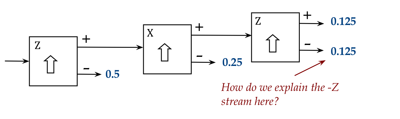
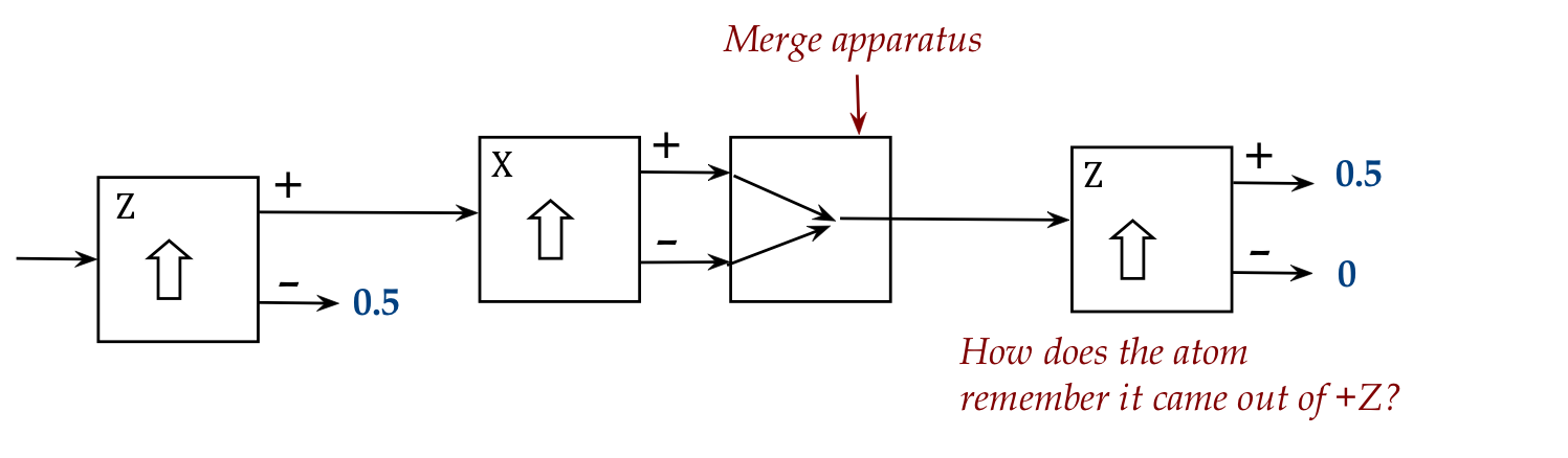
Consider the first experiment:
- The stream of atoms coming out of the + port of the first
(Z-aligned) SG are all in the state \(\kt{z_+}\).
\(\rhd\)
This is how measurement works
(the state changes to the outcome \(\kt{z_+}\))
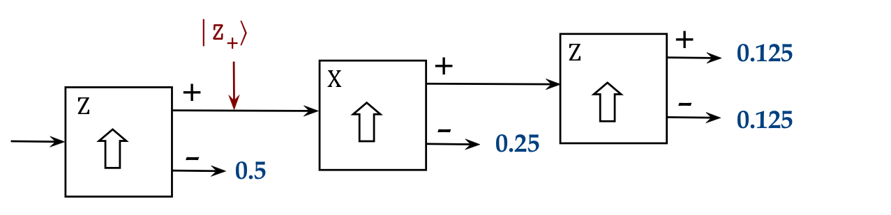
- Now single-atom experiments show that when the
\(\kt{z_+}\) atoms enter the second stage, they come
out of + and - with equal probability.
- Since the second apparatus is described by the basis
\(\kt{x_+}, \kt{x_{-}}\),
we express the input \(\kt{z_+}\) in terms of this basis
$$
\kt{z_+} \eql \alpha \kt{x_+} + \beta \kt{x_{-}}
$$
from which we must have equal probabilities.
- Thus, \(\alpha = \isqt{1} = \beta\):
$$
\kt{z_+} \eql \isqts{1} \kt{x_+} + \isqts{1} \kt{x_{-}}
$$
- This explains the second-stage split.
- When picking off the + stream in the second stage, we know
that the state of those atoms is \(\kt{x_+}\).
- These \(\kt{x_+}\) atoms enter the third stage:
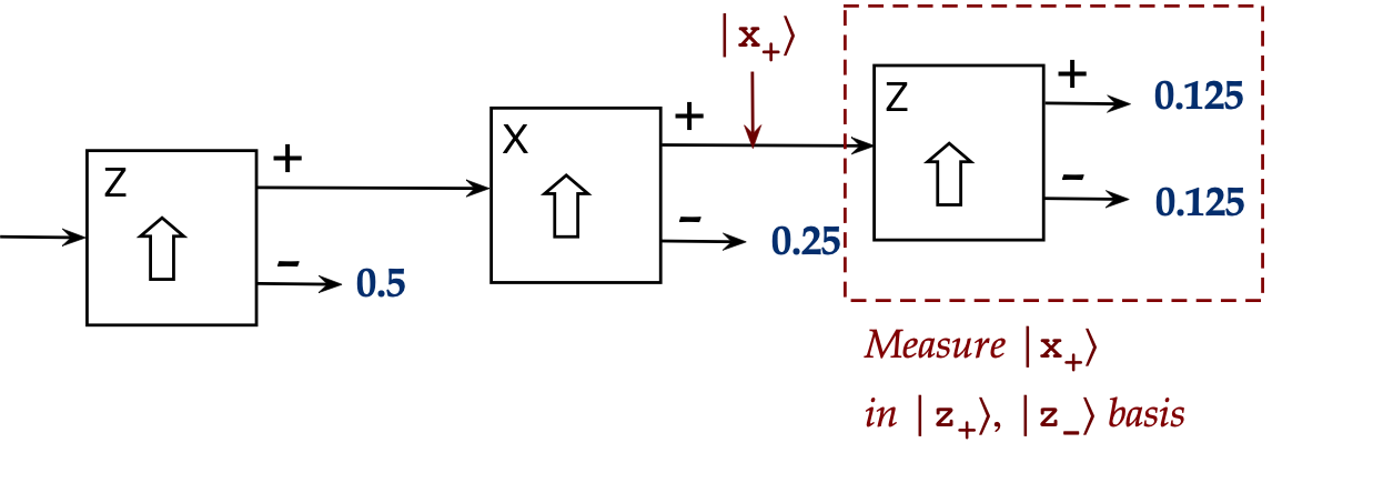
- By symmetry
$$
\kt{x_+} \eql \isqts{1} \kt{z_+} + \isqts{1} \kt{z_{-}}
$$
where \(\kt{z_+}, \kt{z_{-}}\) is the third stage basis.
- This is why we get equal probabilities in the third stage.
Now for the "merged" second stage:
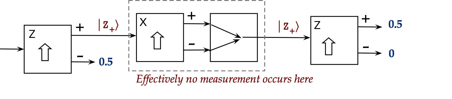
- If the merging is done correctly, no measurement effectively
occurs in the middle.
(We'll make this precise in the next section.)
- This means that the exiting state is the same as the
entering state: \(\kt{z_+}\).
- When \(\kt{z_+}\) is measured in the \(\kt{z_+}, \kt{z_{-}}\)
basis, the outcome is \(\kt{z_+}\) with probability 1!
3.15
Stern-Gerlach explained (Part II)
Let's now revisit the previous section using projectors, which will also give us some practice with them.
First, let's look at the first stage:
- Step 1: Identify the measurement outcomes and then their
projectors:
$$\eqb{
P_{z_+} & \eql \otr{z_+}{z_+} \\
P_{z_-} & \eql \otr{z_-}{z_-}
}$$
- Step 2: Apply each projector to the current state
to obtain projected vectors:
$$\eqb{
P_{z_+}\ksi & \eql \otr{z_+}{z_+} \: \ksi \\
P_{z_-}\ksi & \eql \otr{z_-}{z_-} \: \ksi
}$$
- At this point, we ask: can we calculate not knowing
what \(\ksi\) is?
- No, and it does not matter since we're really using the first
state only to get a stream of \(\kt{z_+}\) atoms.
- We don't know how often they'll occur (because we don't
have enough information about \(\ksi\) to calculate probabilities.
(That's just how this experiment is set up.)
Next, let's look at the second stage:
- The input to measurement is: \(\kt{z_+}\)
- The measurement basis here is \(\kt{x_+}, \kt{x_-}\).
- Step 1: Identify the measurement outcomes and then their
projectors:
$$\eqb{
P_{x_+} & \eql \otr{x_+}{x_+} \\
P_{x_-} & \eql \otr{x_-}{x_-}
}$$
- Step 2: Apply each projector to the current state
to obtain projected vectors:
$$\eqb{
P_{x_+} \kt{z_+} & \eql & \otr{x_+}{x_+} \: \kt{z_+}
& \eql & \inr{x_+}{z_+} \: \kt{x_+} \\
P_{x_-} \kt{z_+} & \eql & \otr{x_-}{x_-} \: \kt{z_+}
& \eql & \inr{x_-}{z_+} \: \kt{x_-} \\
}$$
This time we can calculate the inner products:
$$\eqb{
\inr{x_+}{z_+} & \eql &
\inrs{x_+}{ \isqts{1} \kt{x_+} + \isqts{1} \kt{x_{-}} }
& \eql & \isqts{1} \\
\inr{x_-}{z_+} & \eql &
\inrs{x_-}{ \isqts{1} \kt{x_+} + \isqts{1} \kt{x_{-}} }
& \eql & \isqts{1}
}$$
Thus,
$$\eqb{
P_{x_+} \kt{z_+} & \eql & \inr{x_+}{z_+} \: \kt{x_+}
& \eql & \isqts{1} \kt{x_+} \\
P_{x_-} \kt{z_+} & \eql & \inr{x_-}{z_+} \: \kt{x_-}
& \eql & \isqts{1} \kt{x_-} \\
}$$
- Step 3: Compute the squared magnitude of each projection:
$$\eqb{
\magsq{ P_{x_+} \kt{z_+} } & \eql &
\magsq{ \isqts{1} \kt{x_+} } & \eql &
\magsq{ \isqts{1} } \magsq{ \kt{x_+} } & \eql & \halfsm\\
\magsq{ P_{x_-} \kt{z_+} } & \eql &
\magsq{ \isqts{1} \kt{x_-} } & \eql &
\magsq{ \isqts{1} } \magsq{ \kt{x_-} } & \eql & \halfsm\\
}$$
Which gives us the probabilities for the two outcomes.
- To get accustomed to the projector sandwich, let's repeat this
in that notation:
$$\eqb{
\magsq{ P_{x_+} \kt{z_+} } & \eql &
\swich{z_+}{ P_{x_+} }{z_+} & \eql &
\inr{z_+}{ \isqts{1} \kt{x_+} } & \eql &
\isqts{1} \inr{z_+}{x_+} & \eql & \halfsm\\
\magsq{ P_{x_-} \kt{z_+} } & \eql &
\swich{z_+}{ P_{x_-} }{z_+} & \eql &
\inr{z_+}{ \isqts{1} \kt{x_-} } & \eql &
\isqts{1} \inr{z_+}{x_-} & \eql & \halfsm\\
}$$
- Note: the (un-squared) magnitude or length of each is \(\isqt{1}\).
- Step 4: Compute each normalized projection (divide
each projector vector by its length):
$$\eqb{
\frac{1}{\isqts{1}} \: \isqts{1} \kt{x_+} & \eql & \kt{x_+} \\
\frac{1}{\isqts{1}} \: \isqts{1} \kt{x_-} & \eql & \kt{x_-} \\
}$$
As expected: the normalized projections are the measurement outcomes.
- The third stage analysis is similar, reversing the roles
of X-measurement and Z-measurement.
Now let's look at the second experiment:
- Here, the second stage is different.
- Earlier, we has said that "effectively no measurement occurs".
- Let's look a little deeper:
- The magnetic fields are "on" in the second apparatus.
- Can we really say that they don't cause measurement?
- In fact, they do, but they add up to "no measurement", as we'll now see.
- Projection for this second stage is different.
- What we mean by merging the paths is that
there will be only one projector in effect that is the sum
of the projectors along the two paths:
$$
P_{\smb{merged}} \eql P_{x_+} \: + \: P_{x_-}
$$
In this case,
$$
P_{x_+} \: + \: P_{x_-}
\eql
\otr{x_+}{x_+} \: + \: \otr{x_-}{x_-}
\eql I
$$
(Recall the completeness relation).
- Thus, applying to the input vector \(\kt{z_+}\)
$$\eqb{
P_{\smb{merged}} \kt{z_+}
& \eql & (P_{x_+} \: + \: P_{x_-}) \: \kt{z_+} \\
& \eql & I \: \kt{z_+} \\
& \eql & \kt{z_+} \\
}$$
This is why there's no change of state.
The projector approach will make more sense once we see more examples
in forthcoming modules.
3.16*
Aside: why complex numbers are needed
So far most of our examples have involved real numbers like
\(\isqt{1}\), even when using the Hadamard basis.
One could ask: why do we need complex numbers at all? Why not just
work with real vectors?
We will use the Stern-Gerlach set up to show that complex
numbers arise naturally from the calculations needed to
explain what we saw.
Let's start with an observation:
- Suppose
$$
\kt{w} \eql a_1 \kt{v_1} + a_2 \kt{v_2}
$$
expresses some vector \(\kt{w}\) in some orthonormal 2D basis
\(\kt{v_1}, \kt{v_2}\).
- Write the coefficients in polar form:
$$
\kt{w} \eql r_1e^{i\theta_1} \kt{v_1} + r_2 e^{i\theta_2} \kt{v_2}
$$
- This is global-phase equivalent to:
$$
e^{-i\theta_1} \left(
r_1e^{i\theta_1} \kt{v_1} + r_2 e^{i\theta_2} \kt{v_2} \right)
\eql
r_1 \kt{v_1} + r_2 e^{i\gamma} \kt{v_2}
$$
where \(\gamma = \theta_2 - \theta_1\).
- Thus, every qubit vector can be written equivalently
with a vector whose first coefficient is real.
With this insight, let's look at the Z-to-X measurement:
- Write
$$\eqb{
\kt{x_+} & \eql & \alpha_1 \kt{z_+} + \beta_1 \kt{z_{-}}\\
\kt{x_{-}} & \eql & \alpha_2 \kt{z_+} + \beta_2 \kt{z_{-}}\\
}$$
- From experiments we know that
$$
\magsq{\alpha_1} \eql \frac{1}{2} \eql \magsq{\alpha_2}
$$
and with the insight that we can choose a phase-equivalence where
these are real, it must be that
$$
\alpha_1 \eql \alpha_2 \eql \isqt{1}
$$
- So, now write
$$\eqb{
\kt{x_+} & \eql & \isqts{1} \kt{z_+} + r_1e^{i\gamma_1} \kt{z_{-}}\\
\kt{x_{-}} & \eql & \isqts{1} \kt{z_+} + r_2e^{i\gamma_2} \kt{z_{-}}\\
}$$
- The second coefficient also results in a probability of
\(\frac{1}{2}\), and so
$$
r_1 \eql r_2 \eql \isqts{1}
$$
- Next, experiments have shown that no \(\kt{x_+}\)-state
atom comes out of a \(\kt{x_{-}}\) port, which means these are
orthogonal vectors:
$$
\inr{x_+}{x_{-}} \eql 0
$$
- Expanding from the expressions for each:
$$
\inrh{ \isqts{1} \br{z_+} + \isqts{1} e^{-i\gamma_1} \br{z_{-}} }{
\isqts{1} \kt{z_+} + \isqts{1} e^{i\gamma_2} \kt{z_{-}}
}
\eql 0
$$
Or
$$
e^{i (\gamma_2 - \gamma_1)} + 1 \eql 0
$$
- We can choose \(\gamma_1\) because:
the actual Z-X directions are only relative to each other.
- The most convenient choice is \(\gamma_1 = 0\).
- This implies
$$
e^{i\gamma_2} \eql -1
$$
and therefore
$$\eqb{
\kt{x_+} & \eql & \isqts{1} \kt{z_+} + \isqts{1} \kt{z_{-}}\\
\kt{x_{-}} & \eql & \isqts{1} \kt{z_+} - \isqts{1} \kt{z_{-}}\\
}$$
- So far, no complex numbers.
Next, we need to set up the equations implied by the
third basis: \(\kt{y_+}, \kt{y_{-}}\)
- Write
$$\eqb{
\kt{y_+} & \eql & \alpha_3 \kt{z_+} + \beta_3 \kt{z_{-}}\\
\kt{y_{-}} & \eql & \alpha_4 \kt{z_+} + \beta_4 \kt{z_{-}}\\
}$$
- Orthogonality amongst \(\kt{y_+}, \kt{y_{-}}\) means
$$
\inr{y_+}{y_{-}} = \alpha_3^*\alpha_4 + \beta_3^* \beta_4 \eql 0
$$
- Recall that
$$\eqb{
\kt{x_+} & \eql & \isqts{1} \kt{z_+} + \isqts{1} \kt{z_{-}}\\
\kt{x_{-}} & \eql & \isqts{1} \kt{z_+} - \isqts{1} \kt{z_{-}}\\
}$$
- Thus, we can calculate
$$\eqb{
\inr{y_+}{x_+} & \eql & \isqts{1} ( \alpha_3^* + \beta_3^*)\\
\inr{y_{-}}{x_+} & \eql & \isqts{1} ( \alpha_4^* + \beta_4^*)\\
\inr{y_+}{x_{-}} & \eql & \isqts{1} ( \alpha_3^* - \beta_3^*)\\
\inr{y_{-}}{x_{-}} & \eql & \isqts{1} ( \alpha_4^* - \beta_4^*)\\
}$$
- Next, use these four in the experimental results that
split X-to-Y streams:
$$\eqb{
\inr{y_+}{x_+} \: \inr{x_+}{y_+} & \eql & \halfsm \\
\inr{y_{-}}{x_+} \: \inr{x_+}{y_{-}} & \eql & \halfsm \\
\inr{y_+}{x_{-}} \: \inr{x_{-}}{y_+} & \eql & \halfsm \\
\inr{y_{-}}{x_{-}} \: \inr{x_{-}}{y_{-}} & \eql & \halfsm \\
}$$
- Let's do one of these:
$$\eqb{
\inr{y_+}{x_+} \: \inr{x_+}{y_+}
& \eql &
\isqts{1} (\alpha_3^* + \beta_3^*) \isqts{1} (\alpha_3 + \beta_3) \\
& \eql &
\halfsm (\alpha_3^*\alpha_3 + \beta_3^* \beta_3
+ \alpha_3^*\beta_3 + \alpha_3\beta_3^*) \\
& \eql &
\halfsm (1 + \alpha_3^*\beta_3 + \alpha_3\beta_3^*) \\
}$$
- Equating this to \(\frac{1}{2}\) results in
$$
\alpha_3^*\beta_3 + \alpha_3\beta_3^* \eql 0
$$
or
$$
\alpha_3^*\beta_3 + (\alpha_3^*\beta_3)^* \eql 0
$$
- This is in the form \(z + z^* = 0\),
which implies \(z\)'s real part is 0.
(Try writing \(z=a+ib\) to see why.)
- Recall that we can choose the first coefficient \(\alpha_3\)
to be real.
- This implies \(\beta_3\) cannot be purely real.
\(\rhd\)
\(\beta_3\) must have a non-zero imaginary part.
- Thus, with
$$
\magsq{\alpha_3} \eql \halfsm \eql \magsq{\beta_3}
$$
we can choose
$$
\alpha_3 \eql \isqts{1}
\;\;\;\;\;\;\;
\beta_3 \eql \isqts{i}
$$
- Continuing the analysis, we finally get
$$\eqb{
\kt{y_+} & \eql & \isqts{1} \kt{z_+} + \isqts{i} \kt{z_{-}}\\
\kt{y_{-}} & \eql & \isqts{1} \kt{z_+} - \isqts{i} \kt{z_{-}}\\
}$$
Thus, we have not only explained what necessitated complex numbers,
but we also completed the full analysis of all three SG bases.
3.17*
Aside:
is the set of qubit states a vector space?
Recall that a vector space is closed under addition:
add any two vectors in the vector space and you should
get a vector in that space.
Yet
$$
\ksi \eql \kt{0} + \kt{1}
$$
is not a valid qubit state since it's not unit-length.
What went wrong?
It turns out that a further tweak is needed for mathematical consistency:
- An analogy will help:
- If we want to perform arithmetic (with regular integers)
so that all the integers fall in the range \(0,1,\ldots m-1\),
then we use mod-m with every operation.
- Thus, for example, with \(m=5\)
$$
3 + 4 \;\;\;\; \mbox{ (mod m) } \eql 2
$$
- We can think of this as:
- Perform the operation with regular arithmetic.
- Take the result and compute mod-m.
- Once we do this, all kinds of arithmetic operations
will result in keeping all the results with our
desired set of \(\{0,\ldots, m-1\}\).
- A similar thing can be done with vectors:
- Perform addition, scalar multiplication, or apply an
operator, in the regular way.
- Then, take the result and normalize it.
This way, all normalized results have unit-length.
- This action of normalizing results
in a sort-of vector space called
a projective complex vector space.
- We won't worry about this issue any further.
3.18
Summary
Except for one concept (entanglement), we've used a single
qubit to introduce the main ideas underlying quantum computing:
- A qubit is a 2D complex vector that's normalized.
- There are only two possible interactions with qubits:
- Apply a unitary operator to modify a qubit.
- Measure a qubit.
- Measurement is both intrusive (changes the qubit state)
and probabilistic in outcome
\(\rhd\)
This is what nature does
- Every measurement implies an underlying basis.
- Probabilities are determined by the coefficients of
the qubit vector when the vector is expressed in the
measurement basis.
- The fact that measurement alters state is exploited in
the BB84 key-exchange protocol.
- Unitary operations, on the other hand, alter the state
of a qubit, even though the state can't be "seen".
\(\rhd\)
This is really the key to designing computations
- There is a difference between global
and relative phase when applied to vectors:
$$\eqb{
& \; &
e^{i\theta} \alpha \kt{0} + e^{i\theta} \beta \kt{1}
& \;\;\;\;\;\;\;
& \mbox{Global phase: same as \(\alpha \kt{0} + \beta
\kt{1}\)} \\
& \; &
e^{i\theta} \alpha \kt{0} + \beta \kt{1}
& \;\;\;\;\;\;\;
& \mbox{Relative phase: NOT the same as \(\alpha \kt{0} + \beta \kt{1}\)}
}$$
- We glimpsed how projective measurement works. We will use
this as we build the theory towards multiple qubits.
- A Hermitian operator packages the relevant projectors in a
linear combination, using eigenvalues as the coefficients.
- Hermitians can be analyzed and combined, often using the
sandwich for statistical quantities such as "expected eigenvalue".
- We applied the fundamental theory building blocks to
both polarization and Stern-Gerlach.
- Finally, we saw why complex (as opposed to real)
vectors are essential in explaining physical quantum phenomena.
Don't forget: Module-3 solved problems