What we learned: through the 10 applications
First, let's review the 10 applications from Module 1, in the order
we encountered them there:
- Solving equations.
- This is the founding problem of linear algebra (over 1000
years old).
- We expressed this as \({\bf Ax}={\bf b}\) and saw this
as the question: is there a linear combination of the columns
(they are vectors) of \({\bf A}\) that result in vector \({\bf b}\)?
- With that, we were able to see when you get a solution, when
there's no solution, and when there are multiple.
- Then in Module 5, we developed the RREF approach to get
actual solutions.
- The RREF itself turned out to be the starting point for the
theory of linear algebra, with important concepts like pivot rows/columns.
- Curve fitting.
- If \({\bf Ax}={\bf b}\) cannot be solved because \({\bf b}\)
is not in \({\bf A}\)'s colspace, then we solve approximately
using the "closest" vector in the colspace.
- This is the least-squares method, credited to Gauss when he
sought to fit an ellipse onto data.
- Bezier curves.
- We saw that linear combinations of Bernstein polynomials can be used
to approximate any function.
- When we use two such linear combinations, one each to
determine \(x(t)\) and \(y(t)\), the curve traced by the points
\(x(t), y(t)\) is a Bezier curve, a workhorse of computer graphics.
- The coefficients in the linear combination are conveniently
rendered as control points for the curve, making it easy for
graphic designers to work with.
- 3D view.
- The basic matrix-vector equation can be interpreted as an
expression of coordinates in a different basis (the basis formed
by the columns of the matrix).
- This lets us design matrices to achieve transformations.
- To go the other way, and retrieve coordinates when we know
the transformations, we use the inverses of the matrices involved.
- Compression.
- We saw two types of compression: one from the SVD, and the
other from the DFT.
- The DFT compression throws out high frequencies, making a
bet that (for an audio application), the highest frequencies
won't be missed by the ear.
- The SVD compression throws out terms in the outer-product
that correspond to small \(\sigma_i\)'s on the diagonal of \(\Sigma\).
The reconstruction of the data via the SVD then is approximate,
but close enough.
- Face recognition.
- This part involves recasting data into new coordinates,
using the basis vectors in \({\bf U}\), which is the same thing
as PCA.
- The intuition is that better separation will ease the search problem.
- One trick we had to use: converting a 2D array of pixels
into a 1D array (a vector).
- Google's
page-rank algorithm.
- This models webpage importance with the random-surfer approach.
- The probabilistic solution to the random-surfer is the
highest-eigenvalue eigenvector, when we examined the transition
matrix in the right way.
- There were a few more tricks to use in dealing with large
sizes and dangling nodes.
- Text search.
- This is PCA/SVD applied to documents when documents are
represented as word-vectors.
- Recommendation engine.
- In this problem, we're given a matrix (user-movie ratings)
with missing entries.
- The straightforward way is to try different approximations
with the SVD.
- A slightly more advanced way treats row-column combinations
in the SVD as variables, and optimizes those.
- Audio filtering.
- This involved linear combinations of complex vectors.
- When the vectors are special vectors using the N-th roots of
unity, we get the DFT matrix.
- The DFT is possibly one of the most widely used algorithms
(most often in its optimized FFT form).
What we learned: through \({\bf Ax}={\bf b}\)
- Tuples to vectors:
- We started with wanting to perform arithmetic on groups of
numbers called tuples, as in (1,2,3) + (4,5,-6) = (5,7,-3)
- With a geometric interpretation (arrows) and dot-product,
these became vectors.
- The geometric interpretation of addition is the parallelogram,
and of scalar multiplication is stretching (shrinking, flipping direction).
- The most important operation: linear combination
- We expressed a linear combination of vectors as
$$
{\bf A}{\bf x} \eql {\bf b}
$$
- The scalars are in \({\bf x}\) and the vectors are
columns of \({\bf A}\).
- Coordinates:
- If the columns of \({\bf A}\) are a new basis with
its vectors expressed in
standard coordinates, then the scalars in \({\bf x}\) are
coordinates in that basis.
- Then, the new-basis coordinates of any \({\bf b}\)
in the standard basis (i.e., with standard coordinates)
can be computed through
$$
{\bf x} \eql {\bf A}^{-1}{\bf b}
$$
- When the new basis has orthogonal vectors (as is common in
many graphics applications), this becomes
$$
{\bf x} \eql {\bf A}^{T}{\bf b}
$$
which is how you see it written in graphics books.
- Exact solution:
- We applied row operations in succession to reduce
$$
{\bf A}{\bf x} \eql {\bf b}
$$
to
$$
\mbox{RREF}({\bf A}){\bf x} \eql {\bf b}^\prime
$$
- When \({\bf b}\) is in the colspace of \({\bf A}\),
then \({\bf x}={\bf b}^\prime\) is the solution, and
applying the same operations to \({\bf I}\) produced \({\bf A}^{-1}\)
- An exact solution implies all kinds of nice things:
- \({\bf A}{\bf x}={\bf b}\) has a unique solution.
- \({\bf A}^{-1}\) is unique.
- \({\bf A}{\bf x}={\bf 0}\) has the unique solution
\({\bf x}={\bf 0}\), which is the definition of
linear independence of the columns.
- When exact is not possible:
- When \({\bf b}\) is NOT in the colspace of \({\bf A}\),
we did nonetheless get useful information:
- The pivot rows are a basis for the rowspace.
- The vectors in \({\bf A}\) occupying the same
spots as the pivot columns are a basis for the colspace.
- The dimension of the rowspace and colspace (the rank of the
matrix) is the number of pivots.
- The least-squares method gives us the colspace vector
\({\bf A} \hat{\bf x}\)
closest to \({\bf b}\):
$$
{\bf A} \hat{\bf x}\; \approx \; {\bf b}
$$
This is especially useful when \({\bf A}\) has many more
rows than columns (common in curve-fitting).
- Dot product and angle:
- Since any vector \({\bf u}\) can be first rotated and then
stretched to equal any vector \({\bf v}\), we can write
$$
{\bf v} \cdot {\bf u}
\eql
({\bf B}_\alpha {\bf A}_\theta {\bf u}) \cdot {\bf u} \\
$$
where \({\bf A}_\theta\) performs the rotation and
\({\bf B}_\alpha\) performs the stretch:
\({\bf v} = {\bf B}_\alpha {\bf A}_\theta {\bf u}\)
- This resulted, after some algebraic simplification, into
the very useful relation between dot-product and angle:
$$
{\bf v} \cdot {\bf u}
\eql
|{\bf v}| |{\bf u}| \cos(\theta)
$$
- Orthogonality and projections:
- When \({\bf A}\) is orthogonal
$$
{\bf A}^{-1} \eql {\bf A}^{T}
$$
because \({\bf A}^T{\bf A} = {\bf I}\) since row \(i\) in
\({\bf A}^T\) (which is column \(i\) from \({\bf A}\)) multiplied
by column \(j\) in \({\bf A}\) is zero, and the 1's on the
diagonal come from a column's dot-product with itself.
- The projection of \({\bf u}\) on \({\bf v}\) is
a vector in the direction of \({\bf v}\) that is the
"shadow" of \({\bf u}\):
$$
\mbox{proj}_{\bf v}({\bf u})
\eql
\alpha {\bf v}
$$
where
$$
\alpha \eql
\left(\frac{{\bf u}\cdot {\bf v}}{{\bf v}\cdot {\bf v}} \right)
$$
- By subtracting off projections serially, we got Gram-Schmidt
and the QR decomposition.
- An orthogonal matrix when thought of as a matrix that
transforms vectors has additional nice properties (it preserves
lengths and dot-products).
- Eigenvectors:
- When
$$
{\bf A}{\bf x} \eql \lambda {\bf x}
$$
for some vectors \({\bf x}\), such a vector is called
an eigenvector and the corresponding scalar \(\lambda\) is called
an eigenvalue.
- Repeated application of \({\bf A}\) to an initial vector
results in rapid convergence to the eigenvector with the
highest (in magnitude) eigenvalue, provided the starting
vector is not one of the other eigenvectors.
- For symmetric matrices \({\bf A} = {\bf A}^T\),
the eigenvectors form an orthogonal basis, and
the eigenvalues turn out to be real (possibly negative) numbers.
- If we place these eigenvectors into a matrix \({\bf S}\)
we get the eigendecomposition
$$
{\bf A} \eql {\bf S} {\bf \Lambda} {\bf S}^T
$$
which we exploited in PCA.
- For a special subclass of symmetric matrices, called
positive semidefinite matrices, the eigenvalues
are all negative real numbers, which plays an important role in the SVD.
- SVD/PCA:
- For any (square or non-square) matrix \({\bf A}\)
of rank \(r\),
both \({\bf A}^T {\bf A}\) and \({\bf A} {\bf A}^T\)
are positive semidefinite, meaning their eigenvalues
are nonnegative.
- Put the (orthonormal) eigenvectors of \({\bf A}^T {\bf A}\)
into the matrix \({\bf V}\), and the
(orthonormal) eigenvectors of \({\bf A} {\bf A}^T\) into \({\bf U}\).
Then,
$$
{\bf A} \eql {\bf U} {\bf \Sigma} {\bf V}^T
$$
where \(\Sigma\) is the diagonal matrix of
eigenvalues \(\sqrt{\lambda_1}, \sqrt{\lambda_2},\ldots,\sqrt{\lambda_r}\).
This is the SVD.
- We get even lower-ranked representations (useful in
compression, missing-entry completion) by setting all but the
top few \(\lambda_i\)'s to zero.
- When \({\bf A}\) is a mean-centered
data matrix (multidimensional samples as columns),
then \({\bf A} {\bf A}^T\) is the covariance, whose
eigenvectors \({\bf U}\) can be used for PCA coordinates:
$$
{\bf Y} \eql {\bf U}^{-1} {\bf A}
$$
- Then \({\bf Y}\) is decorrelated with, typically, the highest variance
in the first few dimensions.
- Bezier/DFT:
- These two topics are independent; both involve linear
combinations of "other things" than real-valued vectors.
- The DFT:
- Think of the columns of \({\bf A}\) in \({\bf Ax}={\bf b}\)
as special complex vectors.
- And both \({\bf x}\) and \({\bf b}\) as complex vectors.
- Each element in each of these vectors is some power of
\(\omega=e^{\frac{2\pi i}{N}}\), one of complex N-th roots of 1.
- Then, with the inverse-DFT, \({\bf b}\) is the data, \({\bf A}\)
has the elements of the inverse-DFT matrix, \({\bf b}\) has
the "signal" and \({\bf x}\) is
the vector of Fourier coefficients (containing frequency information).
- This direction goes from frequency to signal, which we
wrote as
$$
{\bf DF} \eql {\bf f}
$$
- In the opposite direction, going from signal to
frequency, \({\bf A}^{-1}\) is converts from data
to Fourier coefficients: \({\bf x}={\bf A}^{-1} {\bf b}\),
which we wrote as
$$
{\bf F} \eql {\bf D}^{-1} {\bf f}
\eql \frac{1}{N}{\bf D}^H{\bf f}
$$
after showing that \({\bf D}\) is orthogonal.
- Bezier:
- This is the one topic that strays from \({\bf Ax}={\bf b}\).
- Here, we defined two functions of this kind:
$$\eqb{
x(t) & \eql & a_0 (1-t)^3 + 3a_1 t (1-t)^2 + 3a_2 t^2(1-t) + a_3 t^3\\
y(t) & \eql & b_0 (1-t)^3 + 3b_1 t (1-t)^2 + 3b_2 t^2(1-t) + b_3 t^3
}$$
where the \(a_i,b_i\) coefficients are the scalars in the
linear combination of special polynomials (called Bernstein polynomials).
- Then, with the really neat approach of parametric
representation of curves, we let
$$\eqb{
x(t) & \eql & \;\;\; \mbox{ x coordinate of the point } (x(t), y(t))\\
y(t) & \eql & \;\;\; \mbox{ y coordinate of the point } (x(t), y(t))
}$$
and plot the points. This is the curve we get.
- As a bonus, if we plot the points \((a_i,b_i)\), moving them
around changes their values and therefore the curve, allowing
visual design with control points.
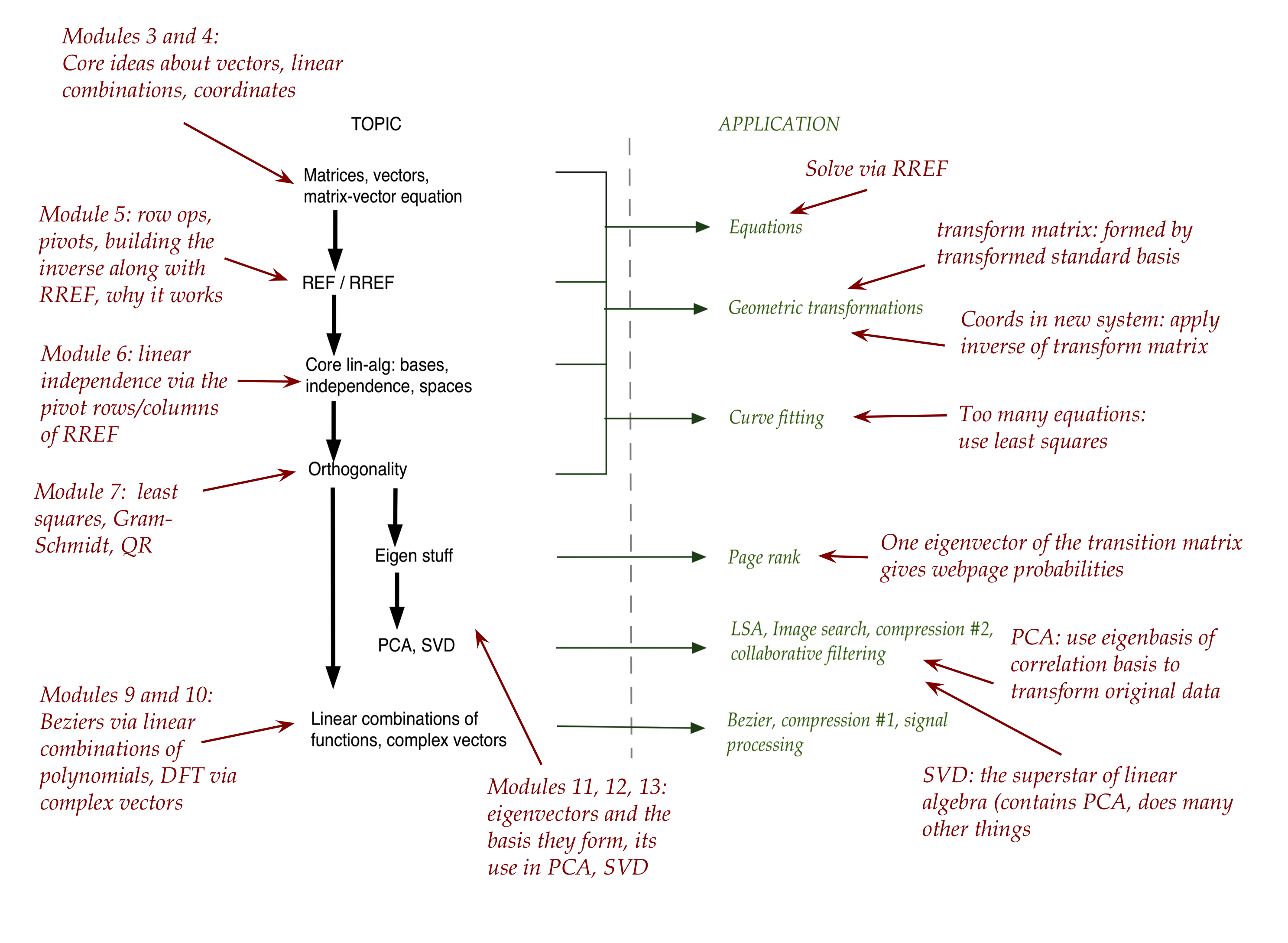
What we learned: through one picture
Look back at Module 1 (Section 1.14) to see all the major topics laid
out in a picture.
Let's annotate that picture to summarize some key lessons:
Where to go from here
Now that you have a basic understanding of linear algebra, what comes
next? Where can you go from here?
- In computer graphics:
- Most transformation matrices are \(4\times 4\), the affine
enhancement for 3D space.
- You can learn how to implement common transformations efficiently,
including, interestingly, one that creates perspective.
- It turns out many curves, including Beziers,
are conveniently represented with groups of matrices.
- See, for example, the basic collection in
a popular graphics tool like Open-GL
- A lot of object geometry also involves matrices, but in a
different (equation-solving) way: to compute intersections to
see whether two moving objects intersect.
- In computer vision and image processing:
- Working with images (or video) requires operations on arrays
of pixels, many of which are described and implemented using
matrices.
- Example applications: filtering, scaling, watermarking,
compression, noise removal.
- One operation worth learning about: convolution.
- Robotics, and graphics involving motion:
- Matrices play a useful role in compactly describing
moving objects, whether inside a 3D world, or actual robots.
- From physics, you might remember that motion involves
velocity (first derivative of position), acceleration (2nd derivative).
When applied to multiple objects, each using a vector to describe
position in 3D space, it's convenient to use matrices called Jacobians
and Hessians for representing derivatives.
- Data science:
- We've already seen regression (curve-fitting) via
least-squares. Many other statistical methods are conveniently
represented with matrix operations.
- Beyond PCA/SVD, there are non-linear methods that are useful
in dimension reduction.
- The missing-entry problem has seen recent advances with
techniques like compressive sensing.
- Graphs:
- In computer science, when we think about graphs, we often
think about popular algorithm like shortest-paths, depth-first
search, and the like.
- Surprisingly, one can represent a graph using an adjacency
matrix (of 0s and 1s), and use its eigenvalues for some graph
problems.
- Quantum computing: the starting point for quantum computing
is a combination of probability, and the linear algebra of complex vectors.
- Computational linear algebra:
- This is a fairly specialized subdiscipline, and quite involved.
- There are sophisticated techniques now for matrix inversion,
SVD, and eigenvalue computations.
- Some of this field involves linear-algebra computations on
specialized hardware (parallel, GPU).
- The most important use: reading
- Many algorithms are presented with
the language of linear algebra.
- Thus, even though the key ideas don't involve linear algebra
concepts (like independence or orthogonality), the presentation
makes use of the compact boldface matrix/vector notation.
What you should consider doing as next steps:
- Mark your calendar a year from now, setting aside 8-10 hours.
- When that time comes, return to the Review section of this
course, and to your own narrative review,
and spend those hours reviewing. How much do you remember?
How much of the modules do you need to re-read? This is how you are
going to build the long-term building blocks that stay with you.
- When you next encounter linear algebra, don't just skim
lightly. Dig a little deeper and see if you can understand finer details.
Lastly: to complete your mathematical toolset for computer science,
spend at least twice the time on probability
that you spent on linear algebra. And I mean
probability, not statistics, although some knowledge of the latter
is useful too.
Probability is bigger, less intuitive, and has far more CS applicability.
See my thoughts on what math is good for CS
and what constitutes
a complete CS education.