Module objectives
By the end of this module, you should be able to
- Describe the SVD.
- Explain the relationship between SVD and eigenvalues.
- Explain how the SVD is used in some applications.
13.0
A review of some ideas
We will review a few key ideas that play a role in the SVD:
- Rowspace vs. column space.
- How a matrix transforms a basis vector of the row space.
- The space spanned by the eigenvectors.
- How a matrix transforms a basis vector of the eigen space.
- The matrix form of eigenvector-eigenvalue pairs:
\({\bf A S}\eql {\bf S \Lambda}\).
- Symmetric matrices have an orthonormal eigenvector basis.
Idea #1: rowspace vs. columnspace
Idea #2: Applying the matrix to one of the rowspace basis vectors:
- What happens when we apply
\({\bf A}\) to a basis vector of the row space?
- For example:
$$
{\bf Ar}_1 \eql
\mat{2 & 1 & 3 & 0 & 3\\
1 & 0 & 1 & 1 & 2\\
3 & 2 & 5 & -1 & 4}
\mat{1\\ 0\\ 1\\ 1\\ 2}
\eql
\mat{11\\ 7\\ 15}
$$
- Since \((11,7,15)\) is in the column space, it can
be expressed as a linear combination of the basis
vectors of the column space:
$$
\vecthree{11}{7}{15} \eql
7 \vecthree{2}{1}{3} - 3 \vecthree{1}{0}{2}
$$
- Thus far, nothing surprising.
- Let's look at another example:
$$
{\bf A}
\eql
\mat{2 & 1 & 3\\
1 & 0 & 1\\
3 & 1 & 2}
$$
- In this case, the RREF is
$$
\mbox{RREF}({\bf A})
\eql
\mat{1 & 0 & 0\\
0 & 1 & 0\\
0 & 0 & 1}
$$
which means:
- The row and column spaces both have dimension 3.
\(\rhd\)
3 vectors are sufficient for the basis.
- Because both are 3D
\(\rhd\)
The same basis will work for both.
- Thus, for example, the standard basis
$$
{\bf e}_1 \; = \; \mat{1\\0\\0}
\;\;\;\;\;\;
{\bf e}_2 \; = \; \mat{0\\1\\0}
\;\;\;\;\;\;
{\bf e}_3 \; = \; \mat{0\\0\\1}
$$
works for both the row space and column space.
- Let's now apply the matrix to one of the row space basis
vectors, e.g., the last one:
$$
\mat{2 & 1 & 3\\
1 & 0 & 1\\
3 & 1 & 2}
\vecthree{0}{0}{1}
\eql
\vecthree{3}{1}{2}
\eql
3 {\bf e}_1
+
1 {\bf e}_2
+
2 {\bf e}_3
$$
- Notice that the result \((3,1,2)\) is, unsurprisingly, a linear
combination of the standard vectors.
Idea #3: eigenvectors as a basis
- Consider the previous \(3\times 3\) example:
$$
{\bf A}
\eql
\mat{2 & 1 & 3\\
1 & 0 & 1\\
3 & 1 & 2}
$$
- It so happens that
$$
{\bf x}_1 \; = \; \mat{0.707\\0\\-0.707}
\;\;\;\;\;\;
{\bf x}_2 \; = \; \mat{0.18\\-0.967\\0.18}
\;\;\;\;\;\;
{\bf x}_3 \; = \; \mat{0.684\\0.255\\0.684}
$$
are eigenvectors with eigenvalues \(-1, -0.372, 5.372\), respectively.
- For example
$$
{\bf Ax}_1
\eql
\mat{2 & 1 & 3\\
1 & 0 & 1\\
3 & 1 & 2}
\mat{0.707\\0\\-0.707}
\eql
-1
\mat{0.707\\0\\-0.707}
$$
- Let's take a closer look at
$$
{\bf Ax}_1 \eql \lambda_1 {\bf x}_1
$$
- We know that \({\bf x}_1\) is in the rowspace of \({\bf A}\).
- Since \({\bf x}_1\) appears on the right, \({\bf x}_1\)
is in the colspace of \({\bf A}\).
- Thus, the size of vectors (number of elements in a vector)
is the same in both the rowspace and colspace.
- This means that, since the rowspace rank is the colspace rank, the
same basis can be used for both the rowspace and colspace.
- Now consider this key observation when \({\bf A}\) is symmetric:
- First, Theorem 12.1 tells us that that the eigenvectors
form a basis.
- A basis for what? For both the column and
row spaces.
Idea #4: Applying the matrix to an eigenbasis vector:
- Recall from above that \({\bf x}_1, {\bf x}_2, {\bf x}_3\)
form a basis for the row and column space.
- Thus, we get the unusual result that, when applying
\({\bf A}\) to a basis vector of the row space,
we get a scalar multiple of a basis vector of the column
space:
$$
{\bf Ax}_i
\eql
\lambda_i {\bf x}_i
$$
Here \({\bf x}_i\) is a vector in both the row and column space bases.
- In other words, \({\bf A}\) maps the row basis
to the column basis when we choose the basis to be the eigenbasis.
- Now, such a thing cannot be possible for an arbitrary
matrix \({\bf A}_{m\times n}\).
- No vector could possibly be in both the row and column space
bases for a non-square matrix.
- However, what might be possible is that there is
some row space basis \({\bf v}_1,{\bf v}_2,\ldots,{\bf v}_r\)
and some column space basis \({\bf u}_1,{\bf u}_2,\ldots,{\bf u}_r\)
such that
$$
{\bf A}{\bf v}_i \eql \mbox{ some multiple of } {\bf u}_i
$$
This is indeed the case, as we'll see in the next section.
- For now, let's look at an example:
- Consider the matrix
$$
{\bf A}
\eql
\mat{2 & 1 & 3 & 0 & 3\\
1 & 0 & 1 & 1 & 2\\
3 & 2 & 5 & -1 & 4}
$$
- It turns out that the RREF is (we saw this earlier):
$$
\mbox{RREF} ({\bf A})
\eql
\mat{{\bf 1} & 0 & 1 & 1 & 2\\
0 & {\bf 1} & 1 & -2 & -1\\
0 & 0 & 0 & 0 & 0}
$$
- So, we need two vectors to form a basis for the rowspace.
- And two vectors to form a basis for the colspace.
- It turns out that
$$
{\bf v}_1 \eql
\mat{0.413\\ 0.238\\ 0.651\\ -0.063\\ 0.587}
\;\;\;\;\;\;\;
{\bf v}_2 \eql
\mat{-0.068\\ 0.344\\ 0.276\\ -0.756\\ 0.479}
$$
is a basis for the rowspace.
- And it turns out that
$$
{\bf u}_1 \eql
\mat{0.528\\ 0.240\\ 0.815}
\;\;\;\;\;\;\;
{\bf u}_2 \eql
\mat{-0.235\\ -0.881\\ 0.411}
$$
is a basis for the colspace.
- Now consider
$$
{\bf Av}_1 \eql
\mat{2 & 1 & 3 & 0 & 3\\
1 & 0 & 1 & 1 & 2\\
3 & 2 & 5 & -1 & 4}
\mat{0.413\\ 0.238\\ 0.651\\ -0.063\\ 0.587}
\eql
0.1104
\mat{0.528\\ 0.240\\ 0.815}
$$
- In other words, it so happens that
$$
{\bf Av}_1 \eql 0.1104 \; {\bf u}_1
$$
- That is, when \({\bf A}\) is applied to a
rowspace basis vector (if the basis is carefully chosen)
the result is a stretched version of a corresponding
colspace basis vector.
- This is a sort-of generalization of what happens with
eigenvectors, and is the foundation of the SVD.
Idea #5: When a matrix \({\bf A}\) has eigenvectors
\({\bf x}_1,{\bf x}_2,\ldots,{\bf x}_n\).
with corresponding
\(\lambda_1,\lambda_2,\ldots,\lambda_n\). Recall that we placed
the \({\bf x}_i\)'s as columns in a matrix \({\bf S}\) and wrote
all the \({\bf A x}_i = \lambda_i {\bf x}_i\) equations in matrix
form as:
$$
{\bf A S}
\eql
{\bf S \Lambda}
$$
Idea #6: A symmetric matrix \({\bf B}_{n\times n}\)
satisfies the conditions for the spectral theorem (Theorem 12.2):
- Theorem 12.2: A real symmetric matrix \({\bf B}\)
can be orthogonally diagonalized. That is, it can be
written as \({\bf B}={\bf S \Lambda} {\bf S}^T\) where
\({\bf \Lambda}\) is the diagonal matrix of eigenvalues
and the columns of \({\bf S}\) are orthonormal eigenvectors.
- We will merely write this as:
$$
{\bf B} \eql {\bf V} {\bf D} {\bf V}^T
$$
This is a mere change in symbols.
- The SVD commonly uses this notation.
13.1
Prelude to the SVD
Consider, for any matrix \({\bf A}_{m\times n}\) the
product \({\bf B}_{n\times n} = {\bf A}^T {\bf A}\):
Now, let's compare the two cases (symmetric, general)
side by side.
| Symmetric matrix \({\bf A}_{n\times n}\) |
General matrix \({\bf A}_{m\times n}\) |
|
Suppose rank = r
|
Suppose rank = r
|
- Since the rank is \(r\) there are r nonzero
real eigenvalues \(\lambda_1,\lambda_2,\ldots,\lambda_r\)
-
There are r orthonormal
eigenvectors \({\bf x}_1,{\bf x}_2,\ldots,{\bf
x}_r\) that form a basis for for both rowspace and colspace.
- For the r nonzero eigenvalues,
\({\bf Ax}_i = \lambda_i {\bf x}_i\)
- Additional \(n-r\) orthonormal vectors can be found
(from the nullspace) so
that \({\bf x}_1,{\bf x}_2,\ldots,{\bf
x}_r, {\bf x}_{r+1},\ldots,{\bf x}_n \) are an orthogonal
basis for \({\bf R}^n\).
|
- There are r orthonormal rowspace basis vectors
\({\bf v}_1,{\bf v}_2,\ldots,{\bf v}_r\)
- And r orthonormal colspace basis vectors
\({\bf u}_1,{\bf u}_2,\ldots,{\bf u}_r\)
- And r nonzero numbers \(\sigma_1,\sigma_2,\ldots,\sigma_r\)
such that \({\bf Av}_i = \sigma_i {\bf u}_i\)
- There are additional orthogonal
vectors (from the nullspace)
\({\bf v}_{r+1},\ldots,{\bf v}_n\)
and \({\bf u}_{r+1},\ldots,{\bf u}_m\)
such that
\({\bf v}_{1},\ldots,{\bf v}_n\) are orthogonal
and a basis for \({\bf R}^n\), and
\({\bf u}_{1},\ldots,{\bf u}_m\) are orthogonal
and a basis for \({\bf R}^m\).
|
13.2
The singular value decomposition (SVD)
There are three forms of the SVD for a matrix \({\bf A}_{m\times n}\)
with rank \(r\):
- The long form, with nullspace bases included.
- The short form (up to rank r)
- The outerproduct form with r terms.
We will look at each in turn, although the latter two are what's
practical in applications.
The long form of the SVD:
- Consider a matrix \({\bf A}_{m\times n}\)
with rank \(r\).
- Recall that
$$
{\bf Av}_i \eql \sigma_i {\bf u}_i
$$
where the \({\bf v}_i\)'s are orthonormal rowspace basis vectors
and \({\bf u}_i\)'s are orthonormal colspace basis vectors.
- And where
$$
\sigma_1 \geq \sigma_2 \geq \ldots \geq \sigma_r \geq
\sigma_{r+1} = \sigma_{r+2} = \ldots = 0.
$$
- Recall: the rank is \(r\) and so
\(\lambda_1, \lambda_2, \ldots, \lambda_r\) are positive
while \(\lambda_{r+1}, \ldots, \lambda_{n}\) are zero.
- \(\sigma_i = \sqrt{\lambda_i}\) (by definition)
- Thus,
\(\sigma_1, \sigma_2, \ldots, \sigma_r\) are positive,
while \(\sigma_{r+1}, \ldots, \sigma_{n}\) are zero.
- Put the \({\bf v}_i\)'s as columns in a matrix \({\bf
V}^\prime_{n\times r}\):
$$
{\bf V}^\prime
\eql
\mat{ & & & \\
\vdots & \vdots & \vdots & \vdots\\
{\bf v}_1 & {\bf v}_2 & \cdots & {\bf v}_r\\
\vdots & \vdots & \vdots & \vdots\\
& & &
}
$$
- Similarly, put the \({\bf u}_i\)'s as columns in a matrix
\({\bf U}^\prime_{m\times r}\):
$$
{\bf U}^\prime
\eql
\mat{ & & & \\
\vdots & \vdots & \vdots & \vdots\\
{\bf u}_1 & {\bf u}_2 & \cdots & {\bf u}_r\\
\vdots & \vdots & \vdots & \vdots\\
& & &
}
$$
In-Class Exercise 4:
How many rows do
\({\bf V}^\prime\) and \({\bf U}^\prime\) have? Why?
- Next, define the diagonal matrix \({\bf \Sigma}_{r\times r}^\prime\)
$$
{\bf \Sigma}^\prime
\eql
\mat{\sigma_1 & 0 & & 0 \\
0 & \sigma_2 & & 0 \\
\vdots & & \ddots & \\
0 & 0 & & \sigma_r
}
$$
- As we did with the spectral decomposition, we can write the
relationship between \({\bf v}_i\)'s and \({\bf u}_i\)'s as
as
$$
{\bf AV}^\prime \eql {\bf U}^\prime{\bf \Sigma}^\prime
$$
In-Class Exercise 5:
Confirm that the matrix multiplications are size-compatible and
that the dimensions on both sides match.
- Now recall that \({\bf A}\) has \(n\)
columns while \({\bf V}^\prime\) has \(r\) columns
- The dim of \({\bf A}\)'s colspace is r.
- The dim of \({\bf A}\)'s nullspace is therefore \(n-r\).
- We can use Gram-Schmidt to find an orthonormal
basis for the nullspace of \({\bf A}\)
- This will need \(n-r\) vectors (the dim of the space).
- Let's call these vectors
\({\bf v}_{r+1},{\bf v}_{r+2},\ldots,{\bf v}_n\).
- Assuming we've found such vectors, we'll expand
the matrix \({\bf V}^\prime\) to add these as columns
and call the resulting matrix \({\bf V}\):
$$
{\bf V}
\eql
\mat{ & & & & & & \\
\vdots & \vdots & \vdots & \vdots & \vdots & \vdots & \vdots \\
{\bf v}_1 & {\bf v}_2 & \cdots & {\bf v}_r &
{\bf v}_{r+1} & \cdots & {\bf v}_n \\
\vdots & \vdots & \vdots & \vdots & \vdots & \vdots & \vdots \\
& & & & & & \\
}
$$
- Note: \({\bf V}\) is \(n\times n\).
- In a similar way, it is possible to expand
\({\bf U}^\prime\) into a matrix \({\bf U}_{m\times m}\).
- Lastly, we'll expand \({\bf \Sigma}^\prime\) into
an \(m\times n\) matrix by adding as many zeroes as necessary.
- We can now expand the earlier relationship
$$
{\bf AV}^\prime \eql {\bf U}^\prime{\bf \Sigma}^\prime
$$
and write it in terms of the expanded matrices:
$$
{\bf AV} \eql {\bf U} {\bf \Sigma}
$$
- Next, because \({\bf V}\) is orthogonal,
we can multiply on the right by \({\bf V}^T\) to give
$$
{\bf A} \eql {\bf U} {\bf \Sigma} {\bf V}^T
$$
In-Class Exercise 6:
Why is this true?
- In other words, any matrix \({\bf A}\) can be decomposed as
$$
{\bf A} \eql
\mbox{ an ortho matrix } \times \mbox{ diagonal matrix }
\times
\mbox{ an ortho matrix }
$$
- This is the singular value decomposition.
- Let's write out the matrix dimensions for clarity:
$$
{\bf A}_{m\times n} \eql {\bf U}_{m\times m} {\bf
\Sigma}_{m\times n} {\bf V}^T_{n\times n}
$$
- We will call this the long form of the SVD.
The short form:
- Because every entry other than the first \(r\) diagonal
values of \({\bf \Sigma}\) are zero, the decomposition can
be reduced to
$$
{\bf A}_{m\times n} \eql {\bf U}_{m\times r} {\bf
\Sigma}_{r\times r} {\bf V}^T_{r\times n}
$$
- The reduced matrices are the ones we started with earlier:
$$
{\bf A}_{m\times n} \eql {\bf U}^\prime_{m\times r} {\bf
\Sigma}^\prime_{r\times r} {\bf V}^{\prime T}_{r\times n}
$$
Let's look at an example to clarify:
- Consider the matrix
$$
{\bf A}
\eql
\mat{2 & 1 & 3 & 0 & 3\\
1 & 0 & 1 & 1 & 2\\
3 & 2 & 5 & -1 & 4}
$$
- In long form, the SVD turns out to be:
$$
\mat{2 & 1 & 3 & 0 & 3\\
1 & 0 & 1 & 1 & 2\\
3 & 2 & 5 & -1 & 4}
\eql
\mat{0.528 & -0.235 & -0.816\\
0.240 & -0.881 & 0.408\\
0.815 & 0.411 & 0.408}
\mat{9.060 & 0 & 0 & 0 & 0\\
0 & 1.710 & 0 & 0 & 0\\
0 & 0 & 0 & 0 & 0}
\mat{0.413 & 0.238 & 0.651 & -0.063 & 0.587\\
-0.068 & 0.344 & 0.276 & -0.756 & -0.479\\
1 & -2 & 1 & 0 & 0\\
1 & -1 & 0 & 1 & 0\\
-1 & -2 & 0 & 0 & 1}
$$
where
$$
{\bf U} \eql
\mat{0.528 & -0.235 & -0.816\\
0.240 & -0.881 & 0.408\\
0.815 & 0.411 & 0.408}
\;\;\;\;\;
{\bf \Sigma} \eql
\mat{9.060 & 0 & 0 & 0 & 0\\
0 & 1.710 & 0 & 0 & 0\\
0 & 0 & 0 & 0 & 0}
\;\;\;\;\;
{\bf V} \eql
\mat{0.413 & -0.068 & 1 & 1 & -1\\
0.238 & 0.344 & -2 & -1 & -2\\
0.651 & 0.276 & 1 & 0 & 0\\
-0.063 & -0.756 & 0 & 1 & 0 \\
0.587 & -0.479 & 0 & 0 & 1}
$$
- Now look at the product \({\bf U\Sigma V}^T\).
- Suppose we first multiply \({\bf U\Sigma}\) in
\(({\bf U\Sigma}){\bf V}^T\).
- In the above example, because the third row of \({\bf
\Sigma}\) is zero,
$$
\mat{0.528 & -0.235 & -0.816\\
0.240 & -0.881 & 0.408\\
0.815 & 0.411 & 0.408}
\mat{9.060 & 0 & 0 & 0 & 0\\
0 & 1.710 & 0 & 0 & 0\\
0 & 0 & 0 & 0 & 0}
\eql
\mat{0.528 & -0.235 \\
0.240 & -0.881 \\
0.815 & 0.411 }
\mat{9.060 & 0 & 0 & 0 & 0\\
0 & 1.710 & 0 & 0 & 0}
\eql
\mat{4.784 & -0.402 & 0 & 0 & 0\\
2.174 & -1.507 & 0 & 0 & 0\\
7.384 & 0.703 & 0 & 0 & 0}
$$
- Furthermore, the resulting matrix has the last three
columns with zeroes.
- This means that we can ignore the last three rows of
\({\bf V}^T\), since those elements will get multiplied by
these zeroes:
$$
\mat{4.784 & -0.402 & 0 & 0 & 0\\
2.174 & -1.507 & 0 & 0 & 0\\
7.384 & 0.703 & 0 & 0 & 0}
\mat{0.413 & 0.238 & 0.651 & -0.063 & 0.587\\
-0.068 & 0.344 & 0.276 & -0.756 & -0.479\\
1 & -2 & 1 & 0 & 0\\
1 & -1 & 0 & 1 & 0\\
-1 & -2 & 0 & 0 & 1}
\eql
\mat{4.784 & -0.402\\
2.174 & -1.507\\
7.384 & 0.703}
\mat{0.413 & 0.238 & 0.651 & -0.063 & 0.587\\
-0.068 & 0.344 & 0.276 & -0.756 & -0.479}
$$
- Thus, the only relevant information is in the first \(r\)
columns of \({\bf V}\) and the first \(r\) rows of \({\bf U}^T\)
- So, if we trimmed all three matrices accordingly, we would
have the short form:
$$
{\bf A} \eql {\bf U}_{m\times r} {\bf \Sigma}_{r\times r} {\bf
V}^T_{r\times n}
$$
Which in our example becomes:
$$
\mat{2 & 1 & 3 & 0 & 3\\
1 & 0 & 1 & 1 & 2\\
3 & 2 & 5 & -1 & 4}
\eql
\mat{0.528 & -0.235 \\
0.240 & -0.881 \\
0.815 & 0.411 }
\mat{9.060 & 0 \\
0 & 1.710}
\mat{0.413 & 0.238 & 0.651 & -0.063 & 0.587\\
-0.068 & 0.344 & 0.276 & -0.756 & -0.479}
$$
- Note: in the short form \({\bf V}_{n\times r}\) has \(r\)
columns.
In-Class Exercise 7:
Download and examine and the code in
SVDExample.java.
Then compile and execute to confirm the above.
Next, the outer-product form:
- Recall:
- Suppose a matrix \({\bf A}\) has columns \({\bf a}_1, {\bf a}_2,\ldots,{\bf a}_k\).
- Suppose \({\bf B}\) has rows \({\bf b}_1, {\bf
b}_2,\ldots,{\bf b}_k\).
- Then, the outerproduct form of \({\bf AB}\) is
$$
{\bf AB} \eql \sum_{i=1}^k {\bf a}_i {\bf b}_i^T
$$
- We will now write the SVD in this form.
- Start by looking at
$$
{\bf U\Sigma}
\eql
\mat{ & & & \\
\vdots & \vdots & \vdots & \vdots\\
{\bf u}_1 & {\bf u}_2 & \cdots & {\bf u}_r\\
\vdots & \vdots & \vdots & \vdots\\
& & &
}
\mat{\sigma_1 & 0 & & 0 \\
0 & \sigma_2 & & 0 \\
\vdots & & \ddots & \\
0 & 0 & & \sigma_r
}
\eql
\mat{ & & & \\
\vdots & \vdots & \vdots & \vdots\\
\sigma_1{\bf u}_1 & \sigma_2{\bf u}_2 & \cdots & \sigma_r{\bf u}_r\\
\vdots & \vdots & \vdots & \vdots\\
& & &
}
$$
- Now, right-multiply by \({\bf V}^T\) for the SVD:
- The rows of \({\bf V}^T\) are the columns of \({\bf V}\).
- These are the vectors
\({\bf v}_1,{\bf v}_2,\ldots,{\bf v}_r\).
- Thus, in outer product form:
$$
{\bf U\Sigma V}^T = \sum_{k=1}^r \sigma_k {\bf u}_k {\bf v}_k^T
$$
- In other words, we can write any matrix \({\bf A}\) as
$$
{\bf A} = \sum_{k=1}^r \sigma_k {\bf u}_k {\bf v}_k^T
$$
where
the \({\bf u}_i\)'s are a basis for the column space
and
the \({\bf v}_i\)'s are a basis for the row space.
- Let's write our running example in outer product form:
$$\eqb{
\sum_{k=1}^r \sigma_k {\bf u}_k {\bf v}_k^T
& \eql &
\sigma_1 {\bf u}_1 {\bf v}_1^T \plss
\sigma_2 {\bf u}_2 {\bf v}_2^T \\
& \eql &
9.060 \mat{0.528\\ 0.240\\ 0.815}
\mat{0.413 & 0.238 & 0.651 & -0.063 & 0.587}
\plss
1.710 \mat{-0.235\\ -0.881\\ 0.411}
\mat{-0.068 & 0.344 & 0.276 & -0.756 & -0.479} \\
& \eql &
9.060 \mat{
0.218 & 0.126 & 0.343 & -0.033 & 0.310\\
0.099 & 0.057 & 0.156 & -0.015 & 0.141\\
0.336 & 0.194 & 0.530 & -0.052 & 0.479}
\plss
1.710 \mat{
0.016 & -0.081 & -0.065 & 0.177 & 0.113\\
0.060 & -0.303 & -0.243 & 0.666 & 0.422\\
-0.028 & 0.141 & 0.114 & -0.311 & -0.197} \\
& \eql &
\mat{
1.973 & 1.138 & 3.111 & -0.303 & 2.808\\
0.898 & 0.518 & 1.416 & -0.138 & 1.278\\
3.048 & 1.758 & 4.806 & -0.468 & 4.337}
\plss
\mat{
0.027 & -0.138 & -0.111 & 0.303 & 0.192\\
0.102 & -0.518 & -0.416 & 1.138 & 0.722\\
-0.048 & 0.242 & 0.194 & -0.532 & -0.337}\\
& \eql &
\mat{2 & 1 & 3 & 0 & 3\\
1 & 0 & 1 & 1 & 2\\
3 & 2 & 5 & -1 & 4}\\
& \eql &
{\bf A}!
}$$
- Notice that storing the \({\bf u}_k\)'s, \({\bf v}_k\)'s,
and \(\sigma_k\)'s might need less space than the whole matrix \({\bf A}\).
- Finally, consider what happens if we discard some of the
terms in the sum
$$
\sum_{k=1}^r \sigma_k {\bf u}_k {\bf v}_k^T
$$
- In our example it turns out that \(r=2\) and so the entire
sum is
$$
\sigma_1 {\bf u}_1 {\bf v}_1^T \plss
\sigma_2 {\bf u}_2 {\bf v}_2^T \\
$$
- Suppose we discard the second part of the sum, and compute
$$\eqb{
{\bf A}^\prime
& \eql &
\sigma_1 {\bf u}_1 {\bf v}_1^T \\
& \eql &
\mat{
1.973 & 1.138 & 3.111 & -0.303 & 2.808\\
0.898 & 0.518 & 1.416 & -0.138 & 1.278\\
3.048 & 1.758 & 4.806 & -0.468 & 4.337}\\
}$$
- Compare this with the original matrix
$$
{\bf A} \eql
\mat{2 & 1 & 3 & 0 & 3\\
1 & 0 & 1 & 1 & 2\\
3 & 2 & 5 & -1 & 4}
$$
- We see that \({\bf A}^\prime\) is a reasonable approximation
$$
{\bf A}^\prime \;\; \approx \;\; {\bf A}
$$
- This is the main idea in using the SVD for compression (next).
13.3
Using the SVD outerproduct form for compression
Recall that any matrix can be expressed in terms of the columns
of \({\bf U}\) and \({\bf V}\), with \(\sigma_k\):
$$
{\bf A} = \sum_{k=1}^r \sigma_k {\bf u}_k {\bf v}_k^T
$$
We'll now explore the idea of using fewer terms in the sum:
$$
{\bf A}_p = \sum_{k=1}^p \sigma_k {\bf u}_k {\bf v}_k^T
$$
where \(p \leq r\).
Why do this?
- First, note that using fewer terms implies an approximation:
\(\rhd\)
The question is: is \({\bf A}_p \approx {\bf A}\)?
- There is a storage advantage to using fewer terms:
- To store \({\bf A}\) we need \(m \times n\) space.
- To store a pair of vectors \({\bf u}_k\) and \({\bf v}_k\),
we need \(m+n\) space.
In-Class Exercise 8:
Why is the storage of the two vectors \(m+n\)?
For \(p\) such terms, what is the total storage,
and when is this less than \(m \times n\)? When is
it greater? Provide some example values of \(m,n\).
- Next, we need to know how accurate the approximation is.
- Or, how small can \(p\) be to get a reasonable approximation?
In-Class Exercise 9:
Download and examine the code in
SVDExample2.java
to confirm that it computes the outerproduct as written above.
Try \(p=1\) and \(p=r\) to compare the resulting matrix
with the original.
How poor an approximation do we get with \(p=1\)?
We'll now explore this notion with images:
Interestingly, there is a nice theoretical result to support this
approach:
Some terminology:
- The numbers \(\sigma_i\) along the diagonal of \({\bf \Sigma}\)
are called the singular values.
- The columns of \({\bf U}\) are called the
left singular vectors
- The columns of \({\bf V}\) are called the
right singular vectors
13.4
Latent semantic analysis (LSA): applying the SVD to text data
Let's begin by understanding two problems with text data:
- The clustering problem: given a collection of documents,
place the documents into topic-related clusters.
- We'll use the term document to mean any blob of text.
- A document could be small (a few words) or very large.
- For this discussion, we'll treat a document as an
unsorted collection of words.
- The search problem: given a collection of documents and
a new query document, find the documents in the collection
that best match the query document.
- The query "document" could just be a group of search terms.
Key ideas in LSA:
- Documents will be converted into numeric vectors.
- Each document will be a column in the data matrix.
- Then we will compute the SVD.
- To sharpen the results, we'll ignore (zero out) some
of the singular values \(\sigma_k\).
- We'll then use the column vectors of the basis \({\bf U}\)
to get the coordinates of the data in this basis.
- Lastly, we'll use the transformed coordinates for both
clustering and search.
Document vectors:
- Let's use an example.
- A document is a collection of words.
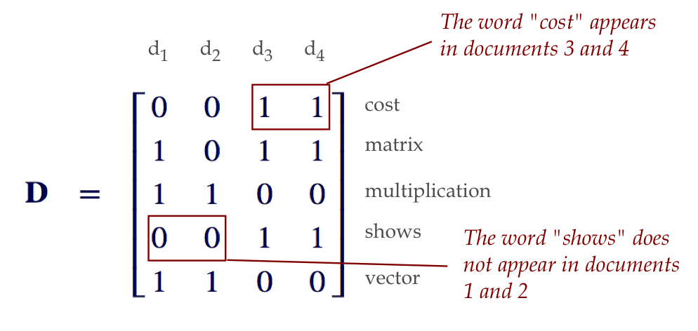
- Consider the following four documents:
- Document 1:
"The multiplication of a matrix with a vector gives a vector"
- Document 2:
"Matrix multiplication is not commutative, but vector dot product is."
- Document 3:
"A balance sheet is like a cost matrix but shows revenue, cost and profit."
- Document 4:
"A cost matrix shows items and costs"
(Yes, they are all very short documents, to make our presentation manageable)
- The first step is to identify a core list of words:
- We'll ignore so-called stop words like "is, a, the" etc.
- Remove all words that occur in only one document.
- We're left with the following 5 words across all four docs:
cost, matrix, multiplication, shows and vector.
- We'll now assign numbers to these words:
      1   cost
      2   matrix
      3   multiplication
      4   shows
      5   vector
- Next, we'll build the word-document matrix \({\bf D}\):
$$
{\bf D}_{ij} =
\left\{
\begin{array}{ll}
1 & \mbox{ if word i is in document j}\\
0 & \mbox{ otherwise}
\end{array}
\right.
$$
- Thus, in our example:
- Note: a more refined version could use word-occurence counts
(how many times a word occurs) instead of just 0 or 1.
- The average of the columns is the vector
$$
{\bf \mu} \eql
\mat{0.5 \\ 0.75 \\ 0.5 \\ 0.5\\ 0.5}
$$
- Then, we center the data by subtracting off the mean column
vector from each column:
$$
{\bf X} \eql
\mat{ -0.5 & -0.5 & 0.5 & 0.5\\
0.25 & -0.75 & 0.25 & 0.25\\
0.5 & 0.5 & -0.5 & -0.5\\
-0.5 & -0.5 & 0.5 & 0.5\\
0.5 & 0.5 & -0.5 & -0.5}
$$
- This will be the data used in the SVD.
- Recall the SVD:
$$
{\bf X} \eql {\bf U} {\bf \Sigma} {\bf V}^T
$$
- Next, let \(r\) be the rank so that:
- The first \(r\) singular values are nonzero:
\(\sigma_1 \geq \sigma_2 \geq \ldots \geq \sigma_r > 0\)
- The others are zero: \(\sigma_{r+1} = \sigma_{r+2} = \ldots = 0\).
- Here, the first \(r\) columns of \({\bf U}\) are a basis
for the data.
- We will use this basis for a change of coordinates.
- And
$$
{\bf U} \eql
\mat{-0.481 & 0.136\\
-0.272 & -0.962\\
0.481 & -0.136\\
-0.481 & 0.136\\
0.481 & -0.136}
\;\;\;\;\;\;
{\bf \Sigma} \eql
\mat{2.070 & 0\\
0 & 0.683}
\;\;\;\;\;\;
{\bf V}^T \eql
\mat{0.432 & 0.564 & -0.498 & -0.498\\
-0.751 & 0.658 & 0.047 & 0.047}
$$
(This is the short form of the SVD).
- Notice that the rank happened to be \(r=2\).
- In other cases, with a higher rank, we might want to zero-out
low singular values and use a small value of \(r\).
- Now, recall that the columns of \({\bf U}\) are the
\({\bf u}_i\) vectors.
\(\rhd\)
They are a basis for the column space of \({\bf X}\).
- Thus, we could re-orient the data to get coordinates
in this new basis.
- How do we change coordinates using the basis \({\bf U}\)?
- Let \({\bf x}_1, {\bf x}_2, \ldots, {\bf x}_n\) be the
columns of the centered data \({\bf X}\).
$$
{\bf X} \eql
\mat{ & & & \\
\vdots & \vdots & \vdots & \vdots\\
{\bf x}_1 & {\bf x}_2 & \cdots & {\bf x}_n\\
\vdots & \vdots & \vdots & \vdots\\
& & &
}
$$
- To change coordinates, we're going to apply
\({\bf U}^T\) to each column:
$$
{\bf y}_i \eql {\bf U}^T {\bf x}_i
$$
- For convenience, we'll now put the \({\bf y}_i\)'s as columns
in a matrix \({\bf Y}\) so that
$$
{\bf Y} \eql {\bf U}^T {\bf X}
$$
- This will allow us to substitute the SVD \({\bf X}={\bf
U\Sigma V}^T\)
$$\eqb{
{\bf Y} & \eql & {\bf U}^T {\bf X}\\
& \eql & {\bf U}^T {\bf U\Sigma V}^T\\
& \eql & {\bf \Sigma V}^T
}$$
as an alternative way to compute the change in coordinates.
- What do we do with the new coordinates, and why would they be useful?
Using the new coordinates for clustering:
- There are many options for clustering, as we've seen in Module 12.
- One approach is to compute the covariance (with changed coordinates)
and identify highly-related documents.
- Note: in computing the covariance, it's more common
to use a ordinal-based covariance like the Spearman correlation
coefficient.
Using the new coordinates for search:
- In the search problem:
- We are given new query document.
- We've already computed the changed coordinates of every
document in the collection.
- We first compute the document vector \({\bf q}\) of
the new query document.
- Then we subtract off the mean:
$$
{\bf q}^\prime \eql {\bf q} - {\bf \mu}
$$
- Then, we get its new coordinates by
$$
{\bf y}^\prime \eql {\bf U}^T {\bf q}^\prime
$$
- Now, we compare against each transformed document
\({\bf y}_i\) to see which one is closest.
- One way to determine closest: find the vector \({\bf y}_i\)
whose angle with \({\bf y}^\prime\) is the least. (This is called cosine-similarity.)
In-Class Exercise 13:
Download and unzip LSA.zip,
then compile and execute LSA.java to
see the above example.
- Read the code to verify the above computations in clustering.
- Change the data set as directed. What are the resulting
sizes of the matrices \({\bf U},{\bf \Sigma}\) and
\({\bf V}^T\)?
- What is notable about the document-document
covariance computed with the changed
coordinates (for each of the two sets of data)?
Why is this approach of using the SVD called latent semantic analysis?
- One interpretation of the new basis vectors \({\bf u}_i\),
that is, the columns of \({\bf U}\) is that each is
a kind of "pseudo" document.
- For example, consider \({\bf u}_1\) in the example above,
along with the corresponding words
    -0.481    cost
    -0.272    matrix
     0.481    multiplication
    -0.481    shows
     0.481    vector
- What interpretation can we assign to these numbers?
- Think of \(-0.481\) as the contribution of the word
"cost" to the pseudo-document \({\bf u}_1\).
- Then, two data vectors that are close are likely to
have similar first coordinate.
\(\rhd\)
Which means the word "cost" has similar value in each of the
two documents.
- Another way to think about it:
- The coordinate transformation highlights shared words.
- Thus, two documents with many shared words will have a small
angle in the new coordinates.
13.5
Image clustering and search using SVD
The ideas of clustering and search above can be applied to
any dataset that can be vectorized.
So, the real question is: how do we turn images into vectors?
Making a vector out of an image:
- First, we'll consider making a vector out of a raw image.
- Let's examine greyscale images.
- A greyscale image is a 2D array of numbers.
- Typically, each number is a value between 0 and 255,
representing intensity.
- Suppose the image is stored in an
array pixels[i][j] of size M rows by N columns.
- A simple way to make this a vector:
- Take the first column of the 2D array, the
numbers
	      pixels[0][0]
              pixels[1][0]
              ...
	      pixels[M-1][0]
- Then append the second column:
	      pixels[0][0]
              pixels[1][0]
              ...
	      pixels[M-1][0]

	      pixels[0][1]
              pixels[1][1]
              ...
	      pixels[M-1][1]
- Then, the third, and so on.
- The resulting vector is the vector representation of a single
image.
- We convert each image into a vector.
- As before, for search or clustering, each image is converted
into a vector and these are transformed into the coordinates
based on the SVD.
- Search and clustering proceed exactly as described for
text once the coordinates are changed.
In-Class Exercise 14:
Download and unzip imageSearch.zip,
then compile and execute ImageSearch.java to
see the above example.
- Read the code to verify the above computations.
- Print the size of \({\bf U}\).
- Examine the files in the eigenImages. What are these
images? What do they correspond to in the SVD?
A caveat:
- We need the image vectors (the analogue of document vectors)
to be comparison-compatible.
- In the case of documents, for example, the second row (thus,
the second component of each document vector) corresponds to the same word.
- But is this true of an image? When applying to face
recognition, we'll need the vector components to be comparable.
- That is, the pixel in position 15 of each vector should be a
pixel that's meaningfully similar across the images.
- What that means is that, in practice,
the images need to be aligned,
and often made coarse-grained before converting into vectors.
13.6
SVD Pseudoinverse and Least Squares
The SVD has turned out to be one of the most useful tools
in linear algebra.
We will list some other applications below.
Application: finding the effective rank of a matrix.
- Sometimes we wish to know the rank of a matrix.
- If a large matrix is low rank, one can look for
a more compact representation.
Recall this about inverses:
- So far, the only inverse we've seen is for a square matrix,
all of whose columns (and rows) are independent.
- The only option we considered when the above isn't true
is the least-squares approach to solve \({\bf Ax}={\bf b}\).
But this requires the columns of \({\bf A}\) to be independent,
and only addresses this problem.
Next, let's turn to finding an approximate inverse
In-Class Exercise 15:
Suppose \({\bf \Sigma}\) is a square diagonal matrix with
\(\sigma_i\) as the i-th entry on the diagonal. What is
the inverse of \({\bf \Sigma}\)?
In-Class Exercise 16:
If \({\bf A}\) is a full-rank square matrix with
SVD \({\bf A}={\bf U\Sigma V}^T\),
then show that \({\bf A}^{-1}={\bf V\Sigma^{-1} U}^T\)
with \({\bf \Sigma}^{-1}\) computed as in the above exercise.
Application: pseudoinverse
- If \({\bf A}\) is not square, we can use the SVD to
define an approximate inverse.
- Clearly, because \({\bf U}\) and \({\bf V}\) (in the
long-form) are
orthogonal and square, they already have inverses.
- The problem is \({\bf \Sigma}\) is not necessarily square
and may not have full rank even if it is.
- But, let's use the idea from the exercise above.
- Define the matrix \({\bf \Sigma}^+\) as follows:
- For each nonzero diagonal entry \(\sigma_k\) in \({\bf \Sigma}\),
let \(\frac{1}{\sigma_k}\) be the corresponding entry in \({\bf \Sigma}^+\)
- Then, the product \({\bf V\Sigma^{+} U}^T\) is somewhat
like an inverse.
- Definition: The pseudoinverse of a matrix \({\bf A}\)
is defined as \({\bf A}^+ = {\bf V\Sigma^{+} U}^T\).
- When \({\bf A}\) is square and invertible, \({\bf A}^+ =
{\bf A}^{-1}\).
- What do we know about \({\bf A}^+\) in general?
- Is the pseudoinverse useful in solving \({\bf Ax}={\bf b}\)
when \({\bf A}\) has no inverse?
- Define the "approximate" solution
$$
{\bf x}^+ \eql {\bf A}^+ {\bf b}
$$
- \({\bf A}^+\) has a nice properties:
- It is equivalent to the true inverse when the true inverse exists.
- \({\bf x}^+\) minimizes \(|{\bf b} - {\bf Ax}|^2\) over
all vectors \({\bf x}\).
- Moreover, \({\bf z}\) is any other solution that
minimizes \(|{\bf b} - {\bf Ax}|^2\), then
\(|{\bf x}^+| \leq |{\bf z}|\).
- The last property implies that the solution from the
pseudoinverse is the "best" in some sense.
- Recall: the RREF is very sensitive to numerical errors.
- Thus, it's best to use \({\bf x}^+\).
- It turns out that computing the SVD can be made numerically robust.
Why use SVD instead of standard least-squares?
- First, let's recall the least-squares approach from Module 7:
$$
\hat{\bf x}
\eql
({\bf A}^T {\bf A})^{-1}
{\bf A}^T {\bf b}
$$
- It turns out that this approach is susceptible to numerical errors.
- How would one use the SVD instead? One approach is to compute the
pseudo-inverse and use it, as shown above.
- A numerically better approach uses this idea:
- For any approximation \(\hat{\bf x}\), consider
the difference between \({\bf A}\hat{\bf x}\) and
the target \({\bf b}\), and substitute the SVD:
$$\eqb{
{\bf A}\hat{\bf x} - {\bf b}
& \eql &
{\bf U\Sigma V}^T \hat{\bf x} - {\bf b} \\
& \eql &
{\bf U} ({\bf \Sigma V}^T \hat{\bf x}) - {\bf U}({\bf U}^T {\bf b})\\
& \eql &
{\bf U} ({\bf \Sigma y} - {\bf c})
}$$
where we've defined \({\bf y}\) and \({\bf c}\) above.
- So, minimizing \({\bf A}\hat{\bf x} - {\bf b}\) is
equivalent to minimizing \({\bf \Sigma y} - {\bf c}\).
- This is a different least-squares problem, but one with a
diagonal matrix (which makes it numerically robust to work with).
Note: The presentation in 13.1, 13.2, and 13.6,
is inspired by this excellent introductory
article:
D.Kalman.
A Singularly Valuable Decomposition: The SVD of a Matrix.
The College Mathematics Journal, Volume 27, Issue 1, 1996.
13.7
The relationship between SVD and PCA: SVD = PCA + more
Both involve finding the eigenvectors of the data matrix multiplied by its
transpose.
Are they merely slight variations of each other?
No! PCA is merely one part (one third) of the SVD.
Let's explain:
- Consider the following data matrix,
$$
{\bf X} \eql
\mat{
5.1 & 4.7 & 7.0 & 6.4 & 6.3 & 5.8\\
3.5,& 3.2 & 3.2 & 3.2 & 3.3 & 2.7\\
1.4 & 1.3 & 4.7 & 4.5 & 6.0 & 5.1\\
0.2 & 0.2 & 1.4 & 1.5 & 2.5 & 1.9}
$$
This is from an actual dataset with samples from three categories.
- Here, each column is a sample of data.
- We have \(m=4\) rows and \(n=6\) columns.
- The number of rows is the dimension of the data.
- Thus the first data point is the first column:
$$
\mat{5.1 \\ 3.5\\ 1.4\\ 0.2}
$$
These are four measurements made of a flowering plant (sepal height,
width, and petal height, width).
- Let's apply PCA and then reflect on its meaning.
In-Class Exercise 17:
Download
PCAExample.java
and
SVDStats.class.
Compile and execute, then examine the code in
PCAExample.java
to confirm that we are applying PCA to the above data.
- Let's review what happens with PCA.
- Compute the mean across the rows:
$$
{\bf\vec{\mu}} = \mat{5.883\\ 3.183\\ 3.833\\ 1.283}
$$
- We first center the data by subtracting \({\bf\vec{\mu}}\)
from each column of the original data to get the centered data:
$$
{\bf X} \eql
\mat{
-0.783 & -1.183 & 1.117 & 0.517 & 0.417 & -0.083\\
0.317 & 0.017 & 0.017 & 0.017 & 0.117 & -0.483\\
-2.433 & -2.533 & 0.867 & 0.667 & 2.167 & 1.267\\
-1.083 & -1.083 & 0.117 & 0.217 & 1.217 & 0.617}
$$
- Next, we compute the covariance matrix (without the \(\frac{1}{n}\))
$$
{\bf C}_{m\times m} \eql {\bf X} {\bf X}^T
$$
Important: this is not \({\bf X}^T {\bf X}\) (which will be
\(n\times n\)).
- Next, because \({\bf C}\) is symmetric, we can diagonalize:
$$
{\bf C} \eql {\bf S \Lambda S}^T
$$
where the eigenvectors are the columns of \({\bf S}\).
- In our example, the eigenvectors turn out to be:
$$
{\bf S} \eql
\mat{
0.314 & -0.897 & -0.103 & -0.294\\
-0.047 & -0.220 & 0.928 & 0.296\\
0.864 & 0.155 & -0.071 & 0.475\\
0.392 & 0.351 & 0.350 & -0.775}
$$
- Lastly, we transform the coordinates of the data using
the eigenvectors as the new basis:
$$\eqb{
{\bf Y} & \eql & {\bf S}^{-1} {\bf X} \\
& \eql & {\bf S}^{T} {\bf X} \\
}$$
- The transformed coordinates give us new decorrelated dimensions.
- To see why, let's compare the two covariance matrices.
- The covariance matrix of the original (centered) data is:
$$
{\bf X}{\bf X}^T \eql
\mat{
3.708 & -0.152 & 7.013 & 2.828\\
-0.152 & 0.348 & -1.147 & -0.512\\
7.013 & -1.147 & 19.833 & 9.043\\
2.828 & -0.512 & 9.043 & 4.268}
$$
It's hard to see whether this is telling us anything, other than
the variance withing the third dimension is higher than the others.
- But look at
$$
{\bf Y}{\bf Y}^T \eql
\mat{
26.546 & -0.000 & 0.000 & -0.000\\
-0.000 & 1.353 & 0.000 & -0.000\\
0.000 & 0.000 & 0.259 & 0.000\\
-0.000 & -0.000 & 0.000 & 0.000}
$$
- The re-oriented data places all the variation in the first modified
dimension.
- The new dimensions are completely de-correlated.
- In the new view, the variation decreases by an order-of-magnitude
from the first to the second, and by another order to the third.
- The interpretation is: only one dimension is really important.
- This makes sense when we plot the first two dimensions
of both the data and the PCA-transformed data:
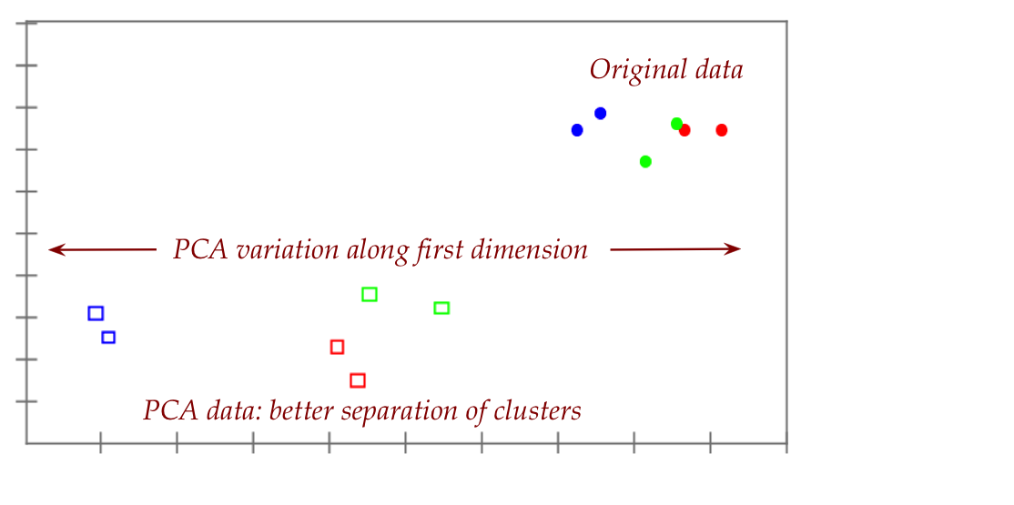
- Here, we happen to know the three categories and are able to show
them in three colors.
- If we didn't know (which is typically the case), it would
harder to discern from the original data.
- Next, let's examine the SVD and observe which part of the
SVD is PCA, when the SVD is in long form:
$$
{\bf X} \eql {\bf U} {\bf \Sigma} {\bf V}^T
$$
Here:
- The columns of \({\bf U}\) are the eigenvectors of
\({\bf XX}^T\).
- The columns of \({\bf V}\) (rows of \({\bf V}^T\))
are the eigenvectors of \({\bf X}^T {\bf X}\).
- In our example, the eigenvectors in \({\bf U}\) are:
$$
{\bf U} \eql
\mat{
0.314 & -0.897 & -0.103 & -0.294\\
-0.047 & -0.220 & 0.928 & 0.296\\
0.864 & 0.155 & -0.071 & 0.475\\
0.392 & 0.351 & 0.350 & -0.775}
$$
Which is exactly the \({\bf S}\) matrix in PCA.
- Finally, let's examine the \({\bf \Sigma}\) matrix:
$$
{\bf \Sigma} \eql
\mat{
5.152 & 0.000 & 0.000 & 0.000\\
0.000 & 1.163 & 0.000 & 0.000\\
0.000 & 0.000 & 0.509 & 0.000\\
0.000 & 0.000 & 0.000 & 0.015}
$$
This tells us the importance of each dimension.
- Note: in the short-form of the SVD, \({\bf U}\) only has
\(r\) columns, and will therefore have fewer columns than
the \({\bf S}\) matrix from PCA.
What do we learn from all of this?
- Think of the SVD as the complete decomposition:
$$
{\bf X} \eql {\bf U} {\bf \Sigma} {\bf V}^T
$$
The SVD
- contains PCA in the \({\bf U}\) part;
- applies to data matrices and other kinds of matrices;
- has many more applications beyond data matrices.
- PCA is so-called because one can go deeper into the
\({\bf U}\) part for data matrices only
and prove that the result decorrelates data between the rows.
- An assumption that's buried inside PCA is that when you go
across a row, the variation is because of noise from column to column.
- If that were not true, then \({\bf X}{\bf X}^T\) is not correlation.
- In PCA we are really interested in correlation between
rows (among the dimensions of the data).
- This assumption is not needed in SVD for its other applications.
- In fact, the SVD applications we've seen, we cared about
correlation amongst the columns (and not the rows).
- One more important point:
- Most often the SVD is in short-form, which means that
\({\bf U}\) in reduced form (only \(r\) columns) is not the
same as \({\bf S}\) in PCA.
- In this case, the new coordinates via SVD, \({\bf Y}={\bf U}^T{\bf
X}\), will be smaller (few components) than the
coordinates from PCA, \({\bf Y}={\bf S}^T{\bf X}\). We saw this in
the latent-semantic analysis section.
Let's now turn to a different application of the SVD, the last
of our canonical examples (from Module 1).
13.8
Using SVD to predict missing data (the Netflix problem)
Consider a matrix where the rows are users and columns are movies:
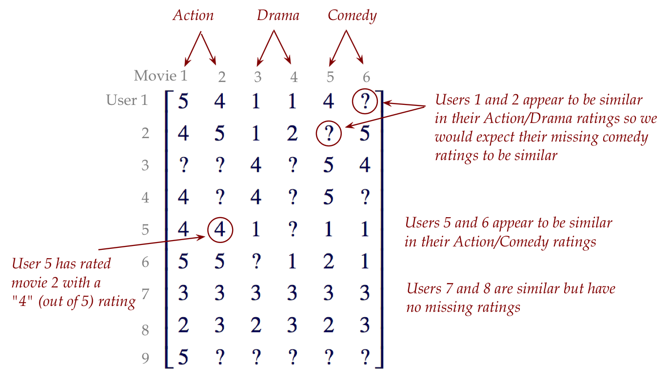
- The rows reflect users, the columns are movies.
- Some entries are missing, indicated with a ?
- We would like to predict these entries as part of developing a
recommendation engine ("if you like X, we think you'll like Y"),
by using the predicted missing entries.
- In real world data, the ratings matrix is typically
very sparse (most entries are missing).
- Many years ago, Netflix announced a million-dollar prize
for anyone who could reasonably predict movie ratings. Most top
performers used some aspects of the SVD.
Let's start with the most direct approach:
- Key ideas:
- Temporarily fill in some values into the missing entries.
- Compute the SVD.
- Find the best low-rank approximation for the actual entries.
- Pseudocode:
    Algorithm: predictMissingRatings (X)
    Input: a ratings matrix X with missing entries
    1.   X' = temporarilyReplaceMissingEntries (X)
    2.   computeSVD (X')
    3.   Σ[m][m] = 0
    3.   for k=m-1 to 1
             // Try the approximation with Σ[k][k] = ... =  Σ[m][m] = 0
    4.       Σ[k][k] = 0
    5.       Y = U Σ VT
             // Compute diff only on non-missing entries of X
    6.       if diff(X,Y) is least so far
    7.           bestY = Y
    8.       endif
    9.   endfor
    10.  return bestY
Note:
- What are the temporary values we could use to replace the
missing entries?
- One option is to use 0.
- Another is to use the average movie rating (in that column).
- Intuition:
- Suppose there is some "true" matrix of all ratings (the one
we are trying to guess).
- Here, the hope is that a low-rank approximation will "capture"
the hidden matrix.
- Remember, by leaving out some singular values (setting
diagonal entries in \({\bf \Sigma}\) to be zero), we can
construct the low-rank approximations.
- The loop merely tries out each such low rank approximation
against the known entries to find the best one.
In-Class Exercise 18:
Download
MovieRatingsSVD.java
and
SVDStats.class.
Compile and execute, then examine the code and output.
Which of the two "temporary value" approaches (zero, or average-movie
rating) do you think is better?
What do do with large matrices:
- Unfortunately, large matrices where most entries are missing
(this was the Netflix data) cause two problems:
- It is difficult to compute the SVD.
- It's empirically known that naive approaches to temporarily
filling in values do not produce good results.
- One of the top performers in the competition used a simpler,
more direct approach, which we'll describe here.
- Let's return to the SVD for a moment:
$$
{\bf X} \eql {\bf U \Sigma V}^T
$$
- Suppose we multiply the latter two matrices and write this as:
$$
{\bf X} \eql {\bf U W}
$$
where \({\bf W} = {\bf \Sigma V}^T\).
- Suppose \({\bf r}_i\)
is the i-th row of \({\bf U}\),
and \({\bf w}_j\)
is the j-th column of \({\bf W}\).
- Then, observe that the i-j-th entry in \({\bf X}\) can be
written as:
$$
{\bf X}_{ij} \eql {\bf r}_i \cdot {\bf w}_j
$$
That is, it is the dot product of row \(i\) in \({\bf U}\)
and column \(j\) in \({\bf W}\).
- This alternative approach asks the following question: why
not treat \({\bf r}_i\) and \({\bf w}_j\) as vector variables
and optimize them directly, without calculating the SVD?
- Suppose we "guessed" values for
\({\bf r}_i\) and \({\bf w}_j\), we could then compute
$$
{\bf Y}_{ij} \eql {\bf r}_i \cdot {\bf w}_j
$$
for all \(i,j\) and use the resulting matrix as the predicted set of
ratings \({\bf Y}\).
- The general, high-level idea is this:
    Algorithm: predictMissingRatings (X)
    Input: a ratings matrix X with missing entries
    1.   for all i,j
    2.      define vector variables ri and wj
    3.   for many iterations
    4.       Try different ri and wj
    5.       Compute Y
    6.       Compute error(X, Y)
    7.       Track the best Y
    8.   endfor
    9.   return best Y
- Of course, rather than try all kinds of
\({\bf r}_i\) and \({\bf w}_j\), we could be smarter about
iterating.
- The smarter way to iterate in an optimization
is to use gradients:
- Consider what this would look like for a simple
function \(f(x)\) with one variable.
- The goal is to find the minimum value \(f(x)\).
- If we start at some "guess" value for \(x\), call it \(x_0\)
- Now iterate as follows:
$$
x_{k+1} \; \leftarrow \; x_{k} - \alpha f^\prime(x_{k})
$$
- What this means:
- At each step, evaluate the gradient with the current
value \(x_{k}\).
- Use it to adjust \(x_{k}\) to change in the opposite
direction (hence the negative sign) of the gradient.
- Opposite, because we want to minimize.
- Why does this work?
- Think of \(f(x)\) as bowl-shaped (the minimum is at the
lowest part of the bowl).
- If the gradient is positive, we are on the upward slope
and need to reduce \(x\) to get to the nadir.
- If the gradient is negative, we need to increase \(x\).
- To learn more about gradient iteration,
see Module
10 of Continuous Algorithms (Section 10.5).
- Now, back to our problem:
consider the i-j-th known value and the current
value of \({\bf r}_i \cdot {\bf w}_j\) and the error
$$
E_{ij} \eql ({\bf X}_{ij} - {\bf r}_i \cdot {\bf w}_j)^2
$$
- We will compute gradients of this and use the gradients
to adjust \({\bf r}_i\) and \({\bf w}_j\).
- In this case, it turns out (from calculus):
$$\eqb{
\frac{\partial E_{ij}}{\partial {\bf r}_i}
& \eql & - 2 {\bf w}_j ({\bf X}_{ij} - {\bf r}_i \cdot {\bf w}_j)\\
\frac{\partial E_{ij}}{\partial {\bf w}_j}
& \eql & - 2 {\bf r}_i ({\bf X}_{ij} - {\bf r}_i \cdot {\bf w}_j)\\
}$$
- So, at each step we update the variables as:
$$\eqb{
{\bf r}_i
& \eql & {\bf r}_i + 2 {\bf w}_j ({\bf X}_{ij} - {\bf r}_i \cdot {\bf w}_j)\\
{\bf w}_j
& \eql & {\bf w}_j + 2 {\bf r}_i ({\bf X}_{ij} - {\bf r}_i \cdot {\bf w}_j)\\
}$$
- Thus, in pseudocode:
    Algorithm: predictMissingRatings (X)
    Input: a ratings matrix X with missing entries
    1.   for all i,j
    2.      define vector variables ri and wj
    3.   for many iterations until converged
    4.       for all i,j
    5.           ri = ri + 2wj(Xij - ri wj)
    6.           wj = wj + 2ri(Xij - ri wj)
    7.       endfor
    8.   endfor

    9.   for all missing i,j
    10.      Xij = riwj
    11.  return X
In-Class Exercise 19:
Download
MovieRatingsIterativeSVD.java,
compile and execute, then examine the code and output.
How does the output compare to the regular SVD?