\(
\newcommand{\blah}{blah-blah-blah}
\newcommand{\eqb}[1]{\begin{eqnarray*}#1\end{eqnarray*}}
\newcommand{\eqbn}[1]{\begin{eqnarray}#1\end{eqnarray}}
\newcommand{\bb}[1]{\mathbf{#1}}
\newcommand{\mat}[1]{\begin{bmatrix}#1\end{bmatrix}}
\newcommand{\nchoose}[2]{\left(\begin{array}{c} #1 \\ #2 \end{array}\right)}
\newcommand{\defn}{\stackrel{\vartriangle}{=}}
\newcommand{\rvectwo}[2]{\left(\begin{array}{c} #1 \\ #2 \end{array}\right)}
\newcommand{\rvecthree}[3]{\left(\begin{array}{r} #1 \\ #2\\ #3\end{array}\right)}
\newcommand{\rvecdots}[3]{\left(\begin{array}{r} #1 \\ #2\\ \vdots\\ #3\end{array}\right)}
\newcommand{\vectwo}[2]{\left[\begin{array}{r} #1\\#2\end{array}\right]}
\newcommand{\vecthree}[3]{\left[\begin{array}{r} #1 \\ #2\\ #3\end{array}\right]}
\newcommand{\vecfour}[4]{\left[\begin{array}{r} #1 \\ #2\\ #3\\ #4\end{array}\right]}
\newcommand{\vecdots}[3]{\left[\begin{array}{r} #1 \\ #2\\ \vdots\\ #3\end{array}\right]}
\newcommand{\eql}{\;\; = \;\;}
\definecolor{dkblue}{RGB}{0,0,120}
\definecolor{dkred}{RGB}{120,0,0}
\definecolor{dkgreen}{RGB}{0,120,0}
\newcommand{\bigsp}{\;\;\;\;\;\;\;\;\;\;\;\;\;\;\;\;\;\;\;\;\;\;\;\;}
\newcommand{\plss}{\;\;+\;\;}
\newcommand{\miss}{\;\;-\;\;}
\newcommand{\implies}{\Rightarrow\;\;\;\;\;\;\;\;\;\;\;\;}
\)
Module 10: Linear Combinations of Other Objects
Part II: Trigonometric polynomials and complex vectors
10.0
Key ideas in this module (and some review)
First, before proceeding:
- Review complex numbers from
Module 2.
\(\rhd\)
You need to be reasonably comfortable with complex numbers for
this module
Let's preview at a high level the key ideas:
10.1
Approximating any function using trignometric functions
First, let's review \(\sin(t)\):
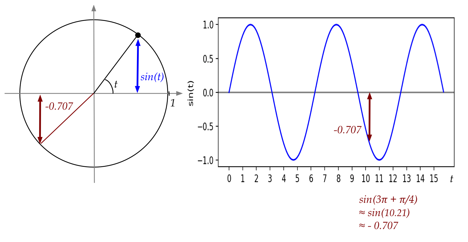
- Think of a dot rotating forever around the unit circle, at 1
radian per second.
- After \(t\) seconds, the angle from the start is \(t\) radians.
- Then
$$
\sin(t) \eql \mbox{height after rotating t radians}
$$
- Example: after one full rotation (\(2\pi\))
and a further rotation of \(\pi + \pi/4\)
$$
t \eql 3\pi + \frac{\pi}{4}
$$
- So,
$$\eqb{
\sin(t) & \eql & \sin(3\pi + \frac{\pi}{4}) \\
& \approx & \sin(10.21) \\
& \approx & -0.707
}$$
The main goal: express any function \(f(t)\) using a linear
combination of sine's and cosine's.
Before that, let's first understand frequency and period:
- We're used to writing \(\sin(t)\)
- It's sometimes helpful to think of the argument \(t\) as
representing time.
- Here, \(\sin(t)\) has one "up" and "down" (cycle) in the interval
\([0,2\pi]\).
- The period is the length of time for one full cycle.
- The next period is the interval \([2\pi,4\pi]\), then
the next after that is \([4\pi,6\pi]\) etc.
In-Class Exercise 1:
Execute Sin.java to plot
\(\sin(t)\) in \([0,2\pi]\). Then, change the interval to
\([0,4\pi]\) to observe two cycles in this larger interval.
You will also need
Function.java,
and SimplePlotPanel.java.
- Next, we will compress the period to the interval \([0,1]\)
by using the function \(\sin(2\pi t)\).
In-Class Exercise 2:
Plot \(\sin(2\pi n t)\) with \(n=1\)
using Sin2.java.
Then change n to 2 and 3.
- Define the frequency as the number of cycles
per unit time.
\(\rhd\)
The number of cycles in \([0,1]\).
- Thus, if we want more cycles in \([0,1]\) we can
increase the frequency by increasing \(n\) in
\(\sin(2\pi n t)\).
- Lastly, suppose we wish to define a sin cycle so that
the period is some arbitrary \(T\).
In-Class Exercise 3:
Plot \(\sin(\frac{2\pi n t}{T})\)
using Sin3.java.
Then change T to try another period.
And vary n.
- Summary: to create a sine function with period \(T\)
and frequency \(n\) cycles per unit time:
\(\rhd\)
Use \(\sin(\frac{2\pi n t}{T})\).
- What is the intuition?
- First, consider \(n=1\) and \(T=1\).
- In this case, \(\sin(\frac{2\pi n t}{T}) = \sin(2\pi t)\).
- Here, the interval is \([0,1]\).
- As \(t\) varies between \(0\) and \(1\), the argument to
\(\sin\) varies between \(0\) and \(2\pi\).
- This, we know, is exactly one cycle.
- Next, suppose we want to "stretch" this out to a period
\([0,T]\):
- This means, we want the argument to evaluate to
\(\sin(2\pi)\) when \(t=T\).
- This is why we scale by \(T\).
- The result is \(\sin(\frac{2\pi t}{T})\).
- Finally, to squeeze multiple cycles, we "boost" the argument
by the number of cycles: \(\sin(\frac{2\pi nt}{T})\).
- Although we will typically use an integer number of cycles
as the frequency, it's entirely possible to use a fractional
(real) number \(\nu\), as in \(\nu=7.45\) cycles.
\(\rhd\)
We usually write this as \(\sin(\frac{2\pi \nu t}{T})\).
A linear combination:
- We saw earlier that we will need both sine's and cosine's.
\(\rhd\)
With just sine's it is not possible to represent a function
\(f(t)\) where \(f(0) > 0\).
- A general linear combination of sine's and cosine's can be
written as:
$$
f_K(t) \eql a_0 + \sum_{n=1}^K a_n \sin(\frac{2\pi nt}{T})
+ \sum_{n=1}^K b_n \cos(\frac{2\pi nt}{T})
$$
- For a technical convenience, we will actually write this as
$$
f_K(t) \eql \frac{a_0}{2} + \sum_{n=1}^K a_n \sin(\frac{2\pi nt}{T})
+ \sum_{n=1}^K b_n \cos(\frac{2\pi nt}{T})
$$
- Notice:
- The scalars in the linear combination are the \(2K+1\) real numbers:
$$
\frac{a_0}{2}, \;\; a_1,a_2,\ldots,a_K, \;\;b_1,b_2,\ldots,b_K
$$
- Unlike other linear combinations, we are using two symbols
to make clear which ones multiply the sine's and which
multiply the cosine's.
- Also, we've singled out one coefficient, \(\frac{a_0}{2}\)
as a sort of "constant".
- This last one is not as strange, if we consider the case \(n=0\).
- Here, when \(n=0\) the cosine term \(\cos(\frac{2\pi nt}{T})\)
evaluates to \(1\).
- Thus, perhaps the better nomenclature would be
\(\frac{b_0}{2}\), but \(\frac{a_0}{2}\) has stuck.
In-Class Exercise 4:
Compile and
execute FourierExample.java
to observe an unknown "mystery function".
You will also need
MysteryFunction.class.
In-Class Exercise 5:
Add code to
FourierExample2.java
to compute the Fourier sum as directed. Compile and execute,
then view the graphs of the mystery function and the Fourier
approximation side by side. Is this a reasonable approximation?
In-Class Exercise 6:
Remove the high frequencies in the same program
above, that is, set \(a_i=0\) for \(i\geq 5\). This simulates
the removal of high-frequency "noise". Does the the resulting
function capture the "essence" of the mystery function?
What if \(a_i=0\) for \(i\geq 4\)?
Separately, compile and
execute SinSumExample.java
to see a linear combination of sine's approximate a square-ish
looking wave.
Write down the linear combination so that you see it more compactly.
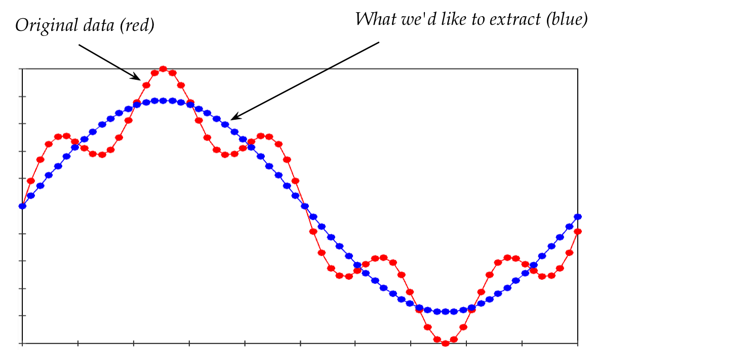
- Often, the goal in a signal processing application is
to capture the essence
\(\rhd\)
We expect that there will be high-frequency noise.
So far, all the variables and coefficients are real numbers.
It turns out to be very convenient to use complex numbers.
Writing the linear combination using complex-number math:
Determining the scalars:
- With Bernstein polynomials, it was rather easy to determine
the scalars.
- With a Fourier series, it is unfortunately not that easy.
- It turns out (we will need additional background for this):
$$
c_n \eql \frac{1}{T} \int_0^T f(t) e^{\frac{2\pi i n t}{T}} dt\\
$$
- In some cases, one can work this out by hand
\(\rhd\)
That turns out to be useful in some problems involving
differential equations.
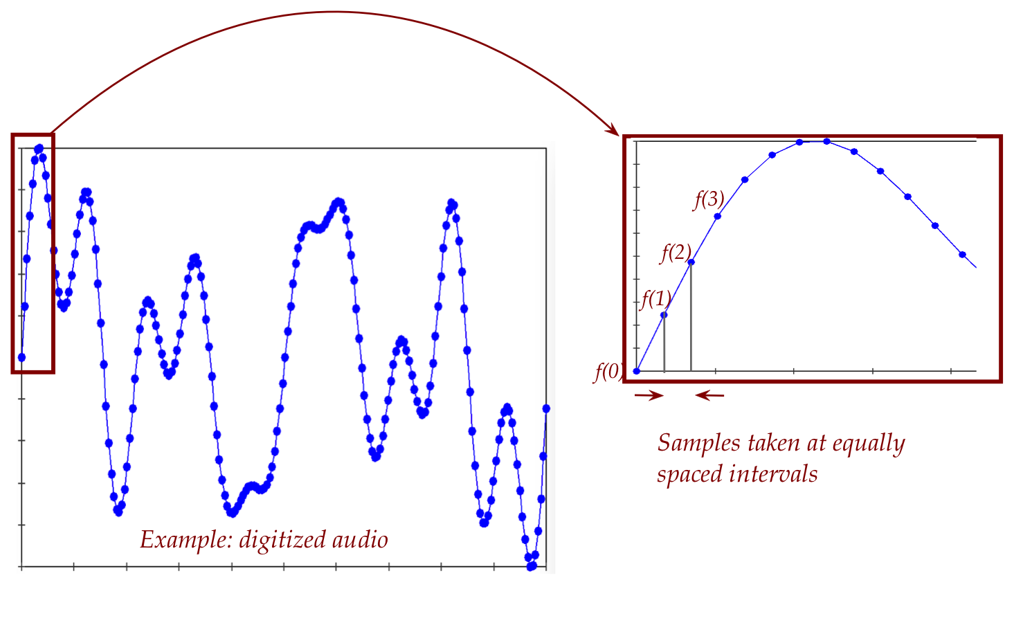
- In practice, when we have data, it is not practical:
- With data, we have no known function \(f(t)\) with which to
perform the integration.
- We'd have to approximate it first to compute the integrals.
- But the goal is to find an approximation.
- This is a sort of double jeopardy.
- Instead, a more practical approach uses discretization.
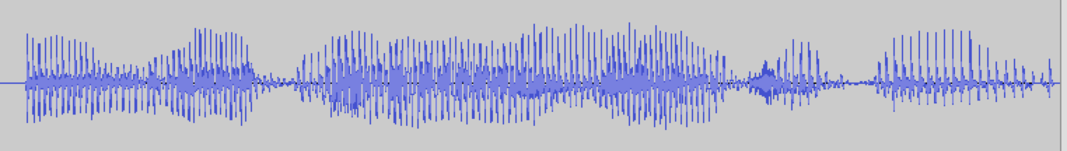
- In practice, real data (such as digitized audio) is discrete:
10.2
Discretizing the linear combination of trigonometric functions
Main ideas in discretization:
- We will discretize in time.
- We'll make two assumptions:
- There are \(N+1\) data points, but such that \(f(0)=f(N)\).
- The period \(T\) is the interval \([0,N-1]\) where
\(N\) is an integer.
- The second one is not as limiting as it might appear:
- If we have some other actual interval with the same
number of data points, we can scale that to the
interval \([0,N-1]\).
- We've implicitly assumed periodicity:
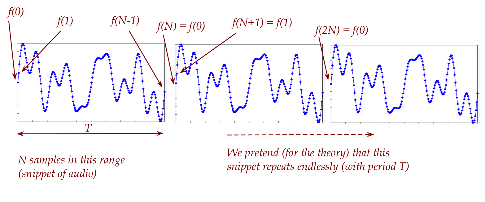
- Since the period is \([0,N-1]\), the next period is \([N,2N-1]\).
- That is, \(f(N) = f(0)\).
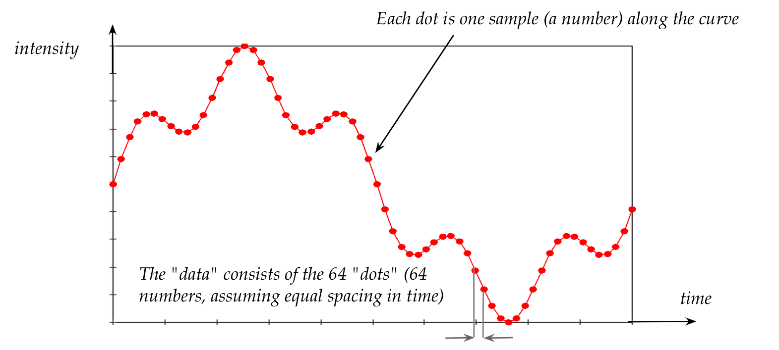
- So, really, there are \(N\) potentially different data
points: \(f(0), f(1), \ldots, f(N-1)\).
An important observation: the number of frequencies are finite (at
most \(N\))
- Consider approximation by the infinite Fourier sum
$$
\sum_{n=-\infty}^{\infty} c_n e^{\frac{2\pi i n t}{N}}
$$
- Here, we're only interested in the value on the
integers \(t=0,1,2,\ldots,N\).
- For the moment, let's expand
$$
e^{\frac{2\pi i n t}{N}} \eql
\cos(\frac{2\pi n t}{N}) + i \sin(\frac{2\pi n t}{N})
$$
- The infinite sum has all of these sine's and cosine's.
- Focus on the sine's for the moment. (The same argument
applies to the cosine's).
- Let's ask the question: can we do without an infinite sum?
- One possibility is to approximate.
- But, as we'll see, we don't have to
\(\rhd\)
We'll use a finite sum that will be exactly the same as the
infinite sum.
- First, let's focus on an infinite linear combination of sine's:
$$
\sum_{n=-\infty}^{\infty} a_n \sin(\frac{2\pi n t}{N})
$$
- For now, let's also focus on \(n \geq 1\):
$$
\sum_{n=1}^{\infty} a_n \sin(\frac{2\pi n t}{N})
$$
- The case \(n=0\) is handled by the constant term.
- We'll sort out negative \(n\) later.
- Separate this out into
$$
\sum_{n=1}^{N} a_n \sin(\frac{2\pi n t}{N})
\plss
\sum_{n=N+1}^{\infty} a_n \sin(\frac{2\pi n t}{N})
$$
- Next, observe that for any integer \(p\)
$$\eqb{
\sin\left( \frac{2\pi(n + pN)t}{N} \right)
& \eql &
\sin\left( \frac{2\pi nt}{N} + 2\pi pt \right) \\
& \eql &
\sin\left( \frac{2\pi nt}{N} \right)
}$$
when \(t\) is an integer.
In-Class Exercise 8:
Why is the last step true?
- The implication is that for any \(q \geq N+1\), the value
of
$$
\sin(\frac{2\pi qt}{N})
$$
is equal to
$$
\sin(\frac{2\pi nt}{N})
$$
for some \(n \leq N\).
- Let's explore this a bit further with an example, because it's not
apparent.
- Consider \(N=10\) and \(n=3\).
- We will examine the value of
$$
\sin(\frac{2\pi n t}{N})
$$
on the integers \(t=0,1,2,\ldots,N\).
- But we'll also plot for all \(t\).
In-Class Exercise 9:
Compile and execute
Periodicity.java
to see the sine above plotted along with values (as dots) on
the integers.
- What would happen if we examine a higher frequency curve
by adding a multiple of \(N\)? That is, we'll plot
$$
\sin(\frac{2\pi (n + pN) t}{N})
$$
In-Class Exercise 10:
Follow the second step in
Periodicity.java
to see both sine's.
- Notice that the points lie on both sine's.
- Thus, as far as (only) the function values on the integers
are concerned, the higher frequency curve has the same
values as the lower frequency.
- Now, in the infinite sum
$$
\sum_{n=1}^{N} a_n \sin(\frac{2\pi n t}{N})
\plss
\sum_{n=N+1}^{\infty} a_n \sin(\frac{2\pi n t}{N})
$$
let's focus on the terms
$$
a_n \sin(\frac{2\pi n t}{N})
\;\;\;\;\;\;\; \mbox{and} \;\;\;\;\;\;\;
a_{n+pN} \sin(\frac{2\pi (n+pN)t}{N})
$$
Since the two sine's have the same values on the integers
(that is, when \(t=0,1,\ldots,N-1\)) we can write this as
$$
(a_n + a_{n+pN}) \sin(\frac{2\pi n t}{N})
$$
In this way, the coefficients of all the sine's whose
value equals
$$
\sin(\frac{2\pi n t}{N})
$$
can be collected into a single coefficient:
$$
(a_n + a_{n+N} + a_{n+2N} + a_{n+3N} + \ldots ) \sin(\frac{2\pi n t}{N})
$$
All of which can be collapsed into a single combined coefficient:
$$
a_n^\prime \sin(\frac{2\pi n t}{N})
$$
- In this manner, we can collapse all corresponding
coefficients for each \(n\leq N\):
$$
\sum_{n=1}^{N} a_n \sin(\frac{2\pi n t}{N})
\plss
\sum_{n=N+1}^{\infty} a_n \sin(\frac{2\pi n t}{N})\\
\eql
\sum_{n=1}^{N} a_n^\prime \sin(\frac{2\pi n t}{N})
$$
The infinite sum is now reduced to an equivalent finite sum!
- Notice: this only works for \(t\in \{0,1,\ldots,N\}\).
\(\rhd\)
But that's all we're interested in.
- Two more tweaks:
- Since \(\sin(0) = 0\) we'll simply include \(n=0\) in the sum.
- Since \(f(N) = f(0)\), we are really only interested in
\(f(0), f(1), \ldots, f(N-1)\).
Putting these two together, we'll write the sum as
$$
\sum_{n=0}^{N-1} a_n^\prime \sin(\frac{2\pi n t}{N})
$$
- Lastly, remember that we ignored \(n < 0\)?
- Those coefficients can be collapsed for the same reason.
- Observe that
$$\eqb{
\sin\left( \frac{2\pi(n - pN)t}{N} \right)
& \eql &
\sin\left( \frac{2\pi nt}{N} - 2\pi pt \right) \\
& \eql &
\sin\left( \frac{2\pi nt}{N} \right)
}$$
when \(t\) is an integer.
- Which covers all the integers less than 0.
- All the arguments above can be replicated almost verbatim
for cosine's.
- Which means they can be replicated for the complex Fourier
sum.
- What does this (rather long) series of arguments buy us?
- The important implication that a finite periodic function on the
integers, \(f(0), f(1), \ldots, f(j),\ldots, f(N-1)\), can
be represented by the finite sum:
$$\eqb{
f(j) & \eql & \sum_{n=-\infty}^\infty c_n e^{\frac{2\pi i nj}{N}} \\
& \eql & \sum_{n=0}^{N-1} c_n^\prime e^{\frac{2\pi i nj}{N}}
}$$
Here, we have collapsed the coefficients into a finite collection
of complex coefficients \(c_0^\prime, c_1^\prime,\ldots, c_N^\prime\).
-
This is one step in what is now called the Discrete Fourier
Transform, one of the most useful tools in applied math.
10.3
The Discrete Fourier Transform (DFT)
Let's summarize where we are in our reasoning so far:
- We have \(N\) data points: \(f(0), f(1), \ldots, f(N-1)\)
spread over an interval of time \(T\)
- Think of these as a function on the integers from \(0\) to \(N\):
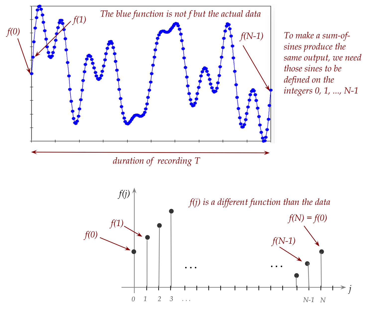
- To make a weighted sum of sines (and cosines) add up to
provide the same function, we need to:
- Ensure the sines and cosines are defined on the integers.
- And that the cycles span the interval \(T\).
- This is why we have terms that "fit" into the interval:
$$
\sin(\frac{2\pi nt}{T})
$$
- Then, Euler's relation helped us neatly write sine/cosine
combinations in terms of exponential-complex numbers:
$$\eqb{
f(t) & \eql & \frac{a_0}{2} + \sum_{n} a_n \sin(\frac{2\pi nt}{T})
+ \sum_{n} b_n \cos(\frac{2\pi nt}{T})\\
& \eql & \sum_{n} c_n e^{\frac{2\pi i n t}{T}}
}$$
(just with different, and complex, coefficients)
- Because high-frequency sines have the same values on the
integers as equivalent low-frequency ones, we were able to
restrict the sum to a finite sum:
$$\eqb{
f(t) & \eql & \sum_{n=-\infty}^\infty c_n e^{\frac{2\pi i nt}{N}} \\
& \eql & \sum_{n=0}^{N-1} c_n^\prime e^{\frac{2\pi i nt}{N}}
}$$
- Since the values of \(t\) are the integers, we'll prefer
using \(j\):
$$
f(j) \eql \sum_{n=0}^{N-1} c_n^\prime e^{\frac{2\pi i nj}{N}}
$$
We'll start with a little re-writing, in a more convenient form:
- Although we used the notation \(f(j)\) to indicate a
function on the integers \(j\), we will rename the numbers
$$
f(0),f(1),\ldots, f(j),\ldots,f(N-1)
$$
to
$$
f_0,f_1,\ldots, f_j,\ldots,f_{N-1}
$$
- Then, for notational symmetry, we'll rename the coefficients
$$
c_0^\prime, c_1^\prime, \ldots, c_{N-1}^\prime
$$
to
$$
F_0, F_1, \ldots, F_{N-1}
$$
so that the sum can be written
$$
f_j \eql \sum_{n=0}^{N-1} F_n e^{\frac{2\pi i nj}{N}}
$$
- Now, because we allow the \(F_n\)'s to be complex,
we must, for symmetry, let the \(f_j\)'s be complex as well.
\(\rhd\)
This is because a complex linear combation can end up being complex.
- In practice, of course, actual data is real-valued.
- We can always write the real number \(x\) as the complex
number \(x + i0\).
- We will in fact get complex "data" when we change the
\(F_n\)'s to achieve some goal (like noise removal).
- So, henceforth, we'll assume that the \(f_j\)'s (the data) are complex.
- Next, use the symbol \(\omega\) to denote the complex number
$$
\omega \eql e^{\frac{2\pi i}{N}}
$$
- With this slight change in notation, the linear combinations
become (one for each \(f_j\)):
$$
f_j \eql \sum_{n=0}^{N-1} F_n \omega^{nj}
$$
In-Class Exercise 11:
Suppose \(N=4\). Write out the unfolded sum for \(f_3\).
- Notice that each \(f_j\) is a linear combination of
numbers (complex numbers).
- However, all our theory so far has been developed for:
- Linear combinations of vectors
- Linear combinations of functions (polynomials).
- One possibility: extend the theory to make it work
for numbers.
In-Class Exercise 12:
What would the theory look like for this extension to
linear combinations of numbers? Explore the meaning of
span, independence, basis, dimension in this context.
- Let's try putting the numbers into vectors to see if
we can make that work.
- The data can be put into a vector quite easily:
$$
{\bf f} \eql \vecfour{f_0}{f_1}{\vdots}{f_{N-1}}
$$
- Next, let's write the linear combinations for
each \(f_j\) one below another:
$$\eqb{
f_0 & \eql & \sum_{n=0}^{N-1} F_n \omega^{n\times 0}
& \eql & F_0 + F_1 + F_2 + F_3 + \ldots + F_{N-1} \\
f_1 & \eql & \sum_{n=0}^{N-1} F_n \omega^{n\times 1}
& \eql & F_0 + F_1 \omega^1 + F_2 \omega^2 +
F_3 \omega^3 + \ldots + F_{N-1} \omega^{N-1} \\
f_2 & \eql & \sum_{n=0}^{N-1} F_n \omega^{n\times 2}
& \eql & F_0 + F_1 \omega^{2} + F_2 \omega^4 +
F_3 \omega^6 + \ldots + F_{N-1} \omega^{2(N-1)} \\
\vdots & \vdots & \vdots & \vdots & \vdots \\
f_{N-1} & \eql & \sum_{n=0}^{N-1} F_n \omega^{n\times (N-1)}
& \eql & F_0 + F_1 \omega^{N-1} + F_2 \omega^{2(N-1)} +
F_3 \omega^{3(N-1)} + \ldots + F_{N-1} \omega^{(N-1)(N-1)}
}$$
In-Class Exercise 13:
Fill in the equation for \(f_3\) above.
- Clearly, this is the same as
$$
\mat{f_0 \\ f_1 \\ f_2 \\ \vdots \\ f_{N-1} }
\eql
F_0 \mat{ 1 \\ 1 \\ 1 \\ \vdots \\ 1}
+ F_1 \mat{ 1 \\ \omega \\ \omega^2 \\ \vdots \\ \omega^{N-1}}
+ F_2 \mat{ 1 \\ \omega^2 \\ \omega^4 \\ \vdots \\ \omega^{2(N-1)}}
+
\ldots
+ F_{N-1} \mat{ 1 \\ \omega^{N-1} \\ \omega^{2(N-1)} \\ \vdots \\ \omega^{(N-1)(N-1)}}
$$
(Think of the above as equations in the \(F_k\) variables.)
- Let's name the vectors above:
$$
{\bf d}_0 \eql \mat{ 1 \\ 1 \\ 1 \\ \vdots \\ 1}
\;\;\;\;\;\;
{\bf d}_1 \eql \mat{ 1 \\ \omega \\ \omega^2 \\ \vdots \\ \omega^{N-1}}
\;\;\;\;\;\;
{\bf d}_2 \eql \mat{ 1 \\ \omega^2 \\ \omega^4 \\ \vdots \\ \omega^{2(N-1)}}
\;\;\;\;\;\;
\ldots
\;\;\;\;\;\;
{\bf d}_{N-1} \eql \mat{ 1 \\ \omega^{N-1} \\ \omega^{2(N-1)} \\ \vdots \\ \omega^{(N-1)(N-1)}}
$$
In-Class Exercise 14:
Write out the elements of \({\bf d}_3\).
- We've now expressed the (complex) data vector \({\bf f}\) as a
linear combination of the (complex) vectors \({\bf d}_n\):
$$
{\bf f} \eql
F_0 {\bf d}_0 + F_1 {\bf d}_1 + F_2 {\bf d}_2 + F_3 {\bf
d}_3 + \ldots + F_{N-1} {\bf d}_{N-1}
$$
- We now cannot resist the urge to put these vectors into
a matrix (as columns, of course). Define
$$
{\bf D} \eql
\mat{ 1 & 1 & 1 & \vdots & 1 \\
1 & \omega & \omega^2 & \vdots & \omega^{N-1} \\
1 & \omega^2 & \omega^4 & \vdots & \omega^{2(N-1)} \\
\vdots & \vdots & \vdots & \vdots & \vdots \\
1 & \omega^{N-1} & \omega^{2(N-1)} & \ldots &
\omega^{(N-1)(N-1)}
}
$$
In-Class Exercise 15:
What is the fourth column of \({\bf D}\)?
- With which the linear combination of vectors can now be
written as
$$
{\bf f} \eql {\bf D} {\bf F}
$$
where \({\bf F}\) is the vector
$$
{\bf F} \eql \vecfour{F_0}{F_1}{\vdots}{F_{N-1}}
$$
- Or, when expanded out:
$$
\mat{f_0 \\ f_1 \\ f_2 \\ \vdots \\ f_{N-1} }
\eql
\mat{ 1 & 1 & 1 & \vdots & 1 \\
1 & \omega & \omega^2 & \vdots & \omega^{N-1} \\
1 & \omega^2 & \omega^4 & \vdots & \omega^{2(N-1)} \\
\vdots & \vdots & \vdots & \vdots & \vdots \\
1 & \omega^{N-1} & \omega^{2(N-1)} & \ldots &
\omega^{(N-1)(N-1)}
}
\mat{F_0 \\ F_1 \\ F_2 \\ \vdots \\ F_{N-1} }
$$
- In which case, if \({\bf D}^{-1}\) exists,
$$
{\bf F} \eql {\bf D}^{-1} {\bf f}
$$
- Terminology:
- The computation of \({\bf F} = {\bf D}^{-1} {\bf f}\) is
called the Discrete Fourier Transform (DFT).
- Going the other way, \({\bf f} = {\bf D} {\bf F}\) is
called the Inverse Discrete Fourier Transform (I-DFT).
- More terminology:
- The matrix \({\bf D}^{-1}\) is called the DFT matrix.
- The matrix \({\bf D}\) is called the inverse-DFT matrix.
Let's step back for a moment and summarize:
- We started with a function \(f(t)\) and its
Fourier representation
$$
f(t) \eql \sum_{n=-\infty}^{\infty} c_n e^{\frac{2\pi i n t}{T}}
$$
- Two reasons led us to discretization:
- The computation of the coefficients is
complicated and inefficient.
- Actual data in applications tends to be discrete
\(\rhd\)
Example: sound is sampled in digital form.
- Then, with \(N\) discrete data or a function discretized
at \(N\) points, we
have \(N\) values (numbers): \(f(0),f(1),f(2),\ldots, f(N-1)\).
- We showed that, because of the properties of sine's and
cosine's
the discretized infinite linear combination
becomes finite
$$
f(j) \eql \sum_{n=0}^{N-1} c_n^\prime e^{\frac{2\pi i nj}{N}}
$$
which we rewrote (change of notation) as:
$$
f_j \eql \sum_{n=0}^{N-1} F_n \omega^{nj}
$$
- Let's write out the equation for each \(j\):
$$\eqb{
f_0 & \eql & \sum_{n=0}^{N-1} F_n \omega^{n\times 0}
& \eql & F_0 + F_1 + F_2 + F_3 + \ldots + F_{N-1} \\
f_1 & \eql & \sum_{n=0}^{N-1} F_n \omega^{n\times 1}
& \eql & F_0 + F_1 \omega^1 + F_2 \omega^2 +
F_3 \omega^3 + \ldots + F_{N-1} \omega^{N-1} \\
f_2 & \eql & \sum_{n=0}^{N-1} F_n \omega^{n\times 2}
& \eql & F_0 + F_1 \omega^{2} + F_2 \omega^4 +
F_3 \omega^6 + \ldots + F_{N-1} \omega^{2(N-1)} \\
\vdots & \vdots & \vdots & \vdots & \vdots \\
f_{N-1} & \eql & \sum_{n=0}^{N-1} F_n \omega^{n\times (N-1)}
& \eql & F_0 + F_1 \omega^{N-1} + F_2 \omega^{2(N-1)} +
F_3 \omega^{3(N-1)} + \ldots + F_{N-1} \omega^{(N-1)(N-1)}
}$$
- Then, we put this in vector form
$$
{\bf f} \eql
F_0 {\bf d}_0 + F_1 {\bf d}_1 + F_2 {\bf d}_2 + F_3 {\bf
d}_3 + \ldots + F_{N-1} {\bf d}_{N-1}
$$
with the understanding that \({\bf f}\) is the data in complex form (zero
imaginary part).
- This expresses a complex vector as a linear combination of
the special vectors
$$
{\bf d}_0 \eql \mat{ 1 \\ 1 \\ 1 \\ \vdots \\ 1}
\;\;\;\;\;\;
{\bf d}_1 \eql \mat{ 1 \\ \omega \\ \omega^2 \\ \vdots \\ \omega^{N-1}}
\;\;\;\;\;\;
{\bf d}_2 \eql \mat{ 1 \\ \omega^2 \\ \omega^4 \\ \vdots \\ \omega^{2(N-1)}}
\;\;\;\;\;\;
\ldots
\;\;\;\;\;\;
{\bf d}_{N-1} \eql \mat{ 1 \\ \omega^{N-1} \\ \omega^{2(N-1)} \\ \vdots \\ \omega^{(N-1)(N-1)}}
$$
We are now led to some burning questions:
- Are the special vectors \({\bf d}_0,{\bf d}_1,\ldots,{\bf d}_{N-1}\)
independent?
- Do they form a basis? A basis for what space?
- How do we compute the coefficients \({\bf F}=(F_0,F_1,\ldots,F_{N-1})\)?
- Why are we doing all this? Why is this useful?
Let's look into some of these questions next.
10.4
Linear independence of \({\bf d}_0,\ldots,{\bf d}_{N-1}\)
Recall the inverse-DFT
$$
{\bf f} \eql {\bf D} {\bf F}
$$
and, for that matter, the DFT itself:
$$
{\bf F} \eql {\bf D}^{-1} {\bf f}
$$
- Here, the matrix \({\bf D}\) has the vectors
\({\bf d}_0,\ldots,{\bf d}_{N-1}\) as columns.
- We want to ask: do these vectors have any special
properties that'll make the matrix \({\bf D}\) "easy" to work with?
We will establish independence in steps:
Now let's return to the proof of orthogonality.
Two useful properties of \(\omega = e^{\frac{2\pi i}{N}}\):
- Property 1: \(\omega^N = 1\).
In-Class Exercise 18:
Show that this is true.
- Property 2: \(\omega^k \neq 1\) if \(1\leq k \leq N-1\).
- This is a bit harder to prove.
- Start by observing that \(\omega^k = e^{\frac{2\pi ik}{N}}\).
In-Class Exercise 19:
Consider the case \(N=8\) and therefore
\(\omega^k = e^{\frac{2\pi ik}{8}}\). Plot the complex numbers
\(\omega^0, \omega^1, \omega^2\) on the complex plane by examining
the angles. Do you see the pattern? Where are the remaining points?
Which ones are not equal to 1?
- Finally, let's get back to
$$
\frac{z^N-1}{z-1} \eql
\frac{\omega^{N^{p-q}}-1}{\omega^{p-q}-1}
$$
- Because of Property 1
$$
\omega^{N^{p-q}}-1 \eql 1^{p-q}-1 \eql 1 - 1 \eql 0
$$
when \(p\neq q\).
- From Property 2, \(\omega^{p-q} \neq 1\).
- Which means that
$$
\frac{z^N-1}{z-1} \eql
\frac{\omega^{N^{p-q}}-1}{\omega^{p-q}-1}
\eql \frac{0}{\mbox{non-zero}} \eql 0
$$
when \(p\neq q\).
10.5
Computing and applying the DFT
We are left with two questions:
- How to compute \({\bf D}^{-1}\)? We need this to get
the coefficients \(F_0,F_1,\ldots,F_{N-1}\)
$$
{\bf F} \eql {\bf D}^{-1} {\bf f}
$$
- Why is this useful?
Let's answer the first one:
- First recall how we computed coefficients in a linear
combination for real vectors:
- To express \({\bf u} \eql x_1{\bf v}_1 + \ldots + x_n{\bf v}_n\)
we solve
$$
\mat{
& & & \\
\vdots & \vdots & \ldots & \vdots \\
{\bf v}_1 & {\bf v}_2 & \ldots & {\bf v}_n\\
\vdots & \vdots & \ldots & \vdots \\
& & &
}
\mat{x_1 \\ x_2\\ x_3 \\ \vdots \\ x_n}
\eql
\mat{u_1 \\ u_2\\ u_3\\ \vdots \\ u_n}
$$
- For this, we compute the RREF etc.
- But the theory of RREFs was developed with real numbers.
- We could develop a generalized theory to solve complex
systems of equations analogous to the one above.
- However, there is a much simpler procedure for the
particular matrix \({\bf D}\).
- Recall that
$$
{\bf D} \eql
\mat{
& & & \\
\vdots & \vdots & \ldots & \vdots \\
{\bf d}_0 & {\bf d}_1 & \ldots & {\bf d}_{N-1}\\
\vdots & \vdots & \ldots & \vdots \\
& & &
}
$$
and that we showed that for columns \(p, q\)
$$
{\bf d}_p \cdot {\bf d}_q \eql
\left\{
\begin{array}{ll}
N & \;\;\;\;\; \mbox{if } p=q\\
0 & \;\;\;\;\; \mbox{if } p\neq q\\
\end{array}
\right.
$$
- Remember: that's the complex (Hermitian) dot product above.
- For any complex matrix \({\bf D}\), define the conjugate
matrix \(\overline{\bf D}\)
to be the matrix you get by taking the conjugate
of each entry of \({\bf D}\).
- That is, the i-j-th element of \(\overline{\bf D}\) is
$$
\overline{\bf D}_{ij} \eql \overline{{\bf D}_{ij}}
$$
- Definition: The Hermitian transpose
of a complex matrix \({\bf D}\) is the matrix
$$
{\bf D}^H \eql (\overline{\bf D})^T
$$
In-Class Exercise 20:
Use the above facts and definitions to show that
\({\bf D}^H {\bf D} = N{\bf I}\).
In-Class Exercise 21:
Then use the above result to show that
\({\bf D}^{-1} = \frac{1}{N} {\bf D}^H\).
- So, finally, we have a way of computing the DFT.
Lastly, let's point out applications:
- First, some application terminology:
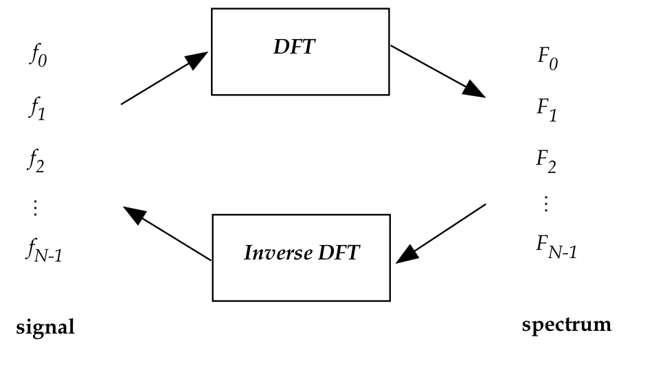
- The collection of input numbers \(f_0,f_1,\ldots,f_{N-1}\) is
called the signal.
- The collection of output numbers \(F_0,F_1,\ldots,f_{N-1}\) is
called the spectrum.
- The signal is the data you get from applications.
- For example, digitized sampling of a musical instrument
will give you a signal.
In-Class Exercise 22:
Download DFTExample.java
and: (1) read the code; (2) then compile and execute to "see"
the music.
You will also need SignalExample.java
How many \(F_0,F_1,\ldots\) values are printed out?
(3) Un-comment the code to print only the significant elements
of the spectrum. Which of \(F_0,F_1,\ldots,F_N\) are significant?
- In this example, we see that most components of the
spectrum are near zero.
\(\rhd\)
Only a few are non-zero.
- Thus, a single sine wave has a spectrum with two non-zero
components.
\(\rhd\)
Both are imaginary in the spectrum.
In-Class Exercise 23:
Why is it unsurprising that for a single sine wave, the
only non-zero components are imaginary?
In-Class Exercise 24:
Download DFTExample2.java,
compile and execute.
Which of \(F_0,F_1,\ldots,F_N\) are significant?
- We will now filter out the "noise" in the second sample.
In-Class Exercise 25:
Download DFTExample3.java
and set the real and imaginary parts of
\(F_5\) and \(F_{59}\) to zero. Then compile and execute.
- This is a classic signal processing application: filtering
to remove noise.
- Note: we have only presented the simplest possible version
of filtering.
- Real music is very complex: even a single note on an
instrument translates to multiple harmonics of changing amplitude.
- Filtering techniques and algorithms are a subspecialty
of digital signal processing (DSP).
- DSP is a big field by itself.
- We also haven't explained the connection between the
"frequency" as in the DFT coefficients and the real-world
frequency of a pure musical note.
\(\rhd\)
This is the domain of the DSP sub-specialty of audio processing.
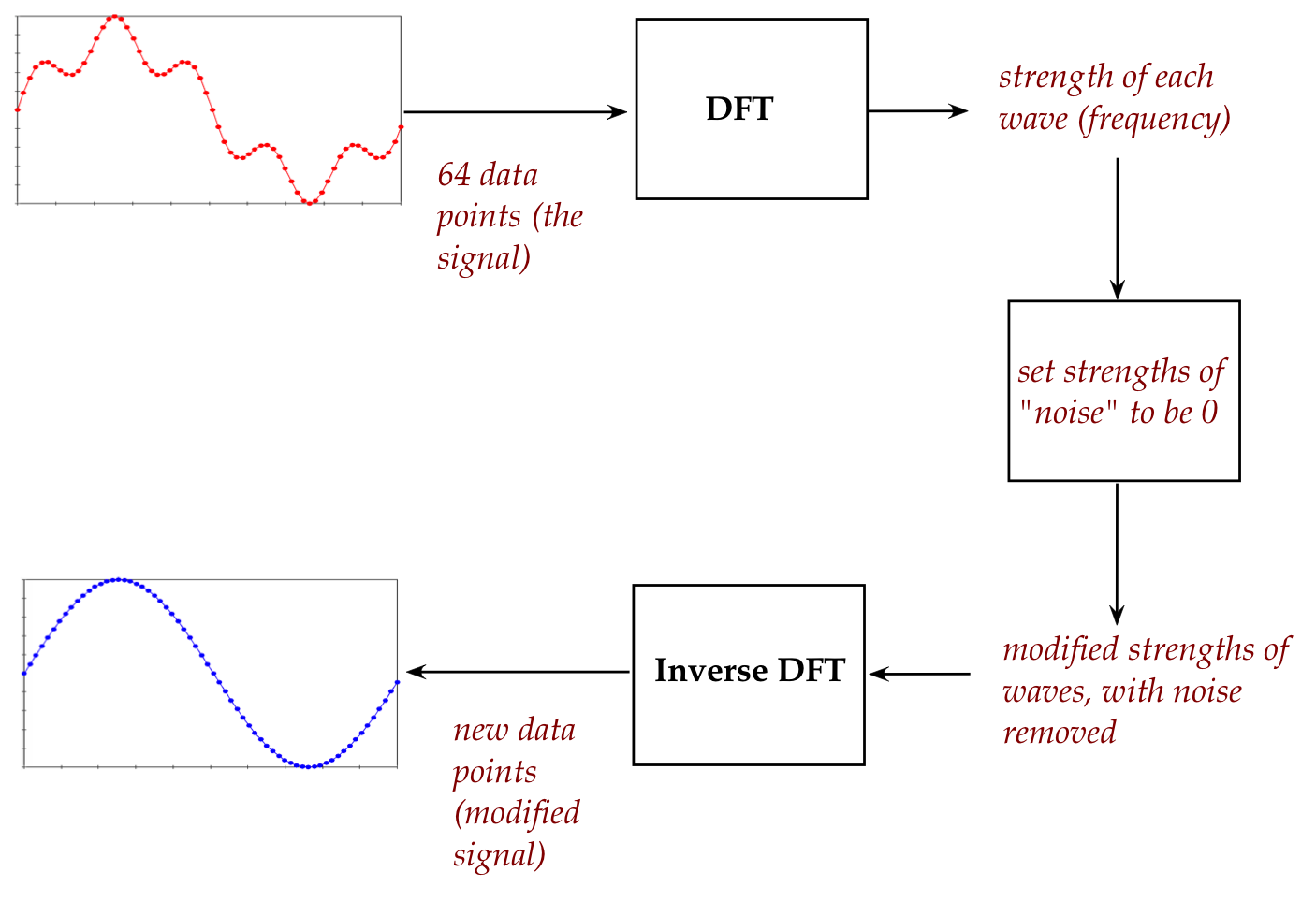
- Filtering is an example of a two-way use of DFT:
- DFT is applied to a signal extract frequency information.
- Then the strengths of frequencies are manipulated.
- After which a new, modified signal is generated as output.
- Example applications include:
- Compression (JPEG).
- Noise removal (your average digital camera).
- Noise cancellation headphones.
- Just about any kind of medical imaging or scientific instrumentation.
- Almost any audio or image processing begins with basic
operations like filtering, noise removal and boosting.
- There are many applications which feature only an analysis
of the DFT output, for example:
- A microphone captures dolphin communication.
- The frequencies are analysed for tell-tale patterns that
are useful in deciphering the communication.
- Other such signature-detection applications include:
- Seismic sensor readings.
- Infrared sensor maps of vegetation to estimate crop efficiency.
In-Class Exercise 26:
Can you find a different and interesting example, with a reference
(URL) to it?
The Fast Fourier Transform (FFT)
10.6
A review and more intuition
We went through many steps in devising the DFT, some of which
can be understandably confusing.
For the purposes of intuition, let's review some key steps:
- We started with Fourier's original hypothesis, that
any periodic function \(f(t)\) with period \(T\)
can be approximated with a linear combination of trig's:
$$
f(t) \eql \frac{a_0}{2} + \sum_{n=1}^\infty a_n \sin(\frac{2\pi nt}{T})
+ \sum_{n=1}^\infty b_n \cos(\frac{2\pi nt}{T})
$$
- We exploited Euler's relation
\(e^{i\theta} = \cos\theta + i\sin\theta\)
to write this as:
$$
\sum_{n=-\infty}^{n=\infty} c_n e^{\frac{2\pi i n t}{T}}
$$
- Next, we restricted the interval to \([0,N]\),
and we only consider the function on the integers \(t=0, 1,\ldots,N-1\).
\(\rhd\)
Here, the periodicity assumption is \(f(0) = f(N)\).
- This is the discretization we perform to make
computations practical.
\(\rhd\)
Any equal-interval discretization can be scaled to the integers.
- This means the approximation becomes
$$
\sum_{n=-\infty}^{\infty} c_n e^{\frac{2\pi i n t}{N}}
$$
for integers \(t\).
- To make this a bit more explicit, we could write this as:
$$
f(j) \eql \sum_{n=-\infty}^{\infty} c_n e^{\frac{2\pi i n j}{N}}
$$
for \(j=0, 1, 2,\ldots,N-1\).
- Further arguments showed that we don't need an infinite
sum because many terms are equal and their coefficients
can be absorbed into earlier ones:
$$
f(j) \eql \sum_{n=0}^{N-1} c_n^\prime e^{\frac{2\pi i nj}{N}}
$$
- We then merely renamed the coefficients to
$$
f(j) \eql \sum_{n=0}^{N-1} F_n^\prime e^{\frac{2\pi i nj}{N}}
$$
- Let's use the symbol
$$
\omega \eql e^{\frac{2\pi i}{N}}
$$
and the symbol
$$
f_j \eql f(j)
$$
- We then get
$$
f_j \eql \sum_{n=0}^{N-1} F_n \omega^{nj}
$$
- When we put the \(f_j\)'s into a complex vector, we
can rewrite the above as
$$
\mat{f_0 \\ f_1 \\ f_2 \\ \vdots \\ f_{N-1} }
\eql
F_0 \mat{ 1 \\ 1 \\ 1 \\ \vdots \\ 1}
+ F_1 \mat{ 1 \\ \omega \\ \omega^2 \\ \vdots \\ \omega^{N-1}}
+ F_2 \mat{ 1 \\ \omega^2 \\ \omega^4 \\ \vdots \\ \omega^{2(N-1)}}
+
\ldots
+ F_{N-1} \mat{ 1 \\ \omega^{N-1} \\ \omega^{2(N-1)} \\ \vdots \\ \omega^{(N-1)(N-1)}}
$$
- Thus, the data vector \(f_0,f_1,\ldots,f_{N-1}\)
is now written as a linear combination of
the basis vectors
$$
{\bf d}_0 \eql \mat{ 1 \\ 1 \\ 1 \\ \vdots \\ 1}
\;\;\;\;\;\;
{\bf d}_1 \eql \mat{ 1 \\ \omega \\ \omega^2 \\ \vdots \\ \omega^{N-1}}
\;\;\;\;\;\;
{\bf d}_2 \eql \mat{ 1 \\ \omega^2 \\ \omega^4 \\ \vdots \\ \omega^{2(N-1)}}
\;\;\;\;\;\;
\ldots
\;\;\;\;\;\;
{\bf d}_{N-1} \eql \mat{ 1 \\ \omega^{N-1} \\ \omega^{2(N-1)} \\ \vdots \\ \omega^{(N-1)(N-1)}}
$$
- We then put these basis vectors into a matrix
$$
{\bf D} \eql
\mat{ 1 & 1 & 1 & \vdots & 1 \\
1 & \omega & \omega^2 & \vdots & \omega^{N-1} \\
1 & \omega^2 & \omega^4 & \vdots & \omega^{2(N-1)} \\
\vdots & \vdots & \vdots & \vdots & \vdots \\
1 & \omega^{N-1} & \omega^{2(N-1)} & \ldots &
\omega^{(N-1)(N-1)}
}
$$
- In matrix notation:
$$
{\bf f} \eql {\bf D} {\bf F}
$$
- Or, to compute the coefficients \(F_j\) (the elements
of the vector \({\bf F}\)
$$
{\bf F} \eql {\bf D}^{-1} {\bf f}
$$
- The fact that the basis is orthogonal (which took some
work to prove) meant that the inverse is easy to compute
\(\rhd\)
It's just the transpose, and so
$$
{\bf F} \eql \frac{1}{N} {\bf D}^{H} {\bf f}
$$
- This, then, is the DFT.
Let's now aim for some intuition:
- The key question is: why does this give us "frequency content"?
- Let's go back to the linear combination
$$
\mat{f_0 \\ f_1 \\ f_2 \\ \vdots \\ f_{N-1} }
\eql
F_0 \mat{ 1 \\ 1 \\ 1 \\ \vdots \\ 1}
+ F_1 \mat{ 1 \\ \omega \\ \omega^2 \\ \vdots \\ \omega^{N-1}}
+ F_2 \mat{ 1 \\ \omega^2 \\ \omega^4 \\ \vdots \\ \omega^{2(N-1)}}
+ F_3 \mat{ 1 \\ \omega^3 \\ \omega^6 \\ \vdots \\ \omega^{3(N-1)}}
+
\ldots
+ F_{N-1} \mat{ 1 \\ \omega^{N-1} \\ \omega^{2(N-1)} \\ \vdots \\ \omega^{(N-1)(N-1)}}
$$
- Here, the \(F_i\)'s are the coordinates of the data in
the transformed basis consisting of the columns above.
- Suppose that \(F_3\) is the dominant coefficient for some
particular data.
\(\rhd\)
We want to ask: what does that mean in terms of frequency?
- It means that the data, after change of coordinates,
is well aligned with the vector
$$
{\bf d}_3 \eql \mat{ 1 \\ \omega^3 \\ \omega^6 \\ \vdots \\ \omega^{3(N-1)}}
$$
- What frequency does this involve?
- Let's look at the elements of the vector:
$$
1, \; \omega^3, \; \omega^6, \; \omega^9, \ldots
$$
Or in terms of the definition of \(\omega\):
$$
e^{\frac{2\pi i(0)}{N}}, \;\;
e^{\frac{2\pi i(3)}{N}}, \;\;
e^{\frac{2\pi i(6)}{N}}, \;\;
e^{\frac{2\pi i(9)}{N}}, \ldots
$$
- We can ignore the first (since it's just 1) and focus
on the frequency
$$
\frac{2\pi}{N} \;\times \; 3
$$
and the function
$$
h(t) \eql \sin (\frac{2\pi 3}{N}t)
\eql \sin (\frac{6\pi}{N}t)
$$
- On the integers, the function takes values
$$\eqb{
h(1) & \eql & \sin (\frac{6\pi}{N}1) \\
h(2) & \eql & \sin (\frac{6\pi}{N}2) \\
h(3) & \eql & \sin (\frac{6\pi}{N}3) \\
}$$
- Thus if the frequency
$$
\frac{6\pi}{N}
$$
is the dominant frequency in the function \(h(t)\), then
the values
$$\eqb{
h(1) & \eql & \sin (\frac{6\pi}{N}1) \\
h(2) & \eql & \sin (\frac{6\pi}{N}2) \\
h(3) & \eql & \sin (\frac{6\pi}{N}3) \\
}$$
will be well represented (high weightage) in the data.
- This is exactly what the Fourier coefficent \(F_3\)
captures.
- So, at last we see the connection between "frequency in the
data" and the appropriate Fourier coefficient.
10.7
The two-dimensional DFT
Consider generalizing the Discrete Fourier Transform to two dimensions:
- First, let's understand what a 2D signal is.
- Note: A 1D signal is an array of complex numbers.
- Thus, a 2D signal should be ... a 2D array of complex numbers.
- One way to visualize this is to seek a simple visualization
of a 1D signal
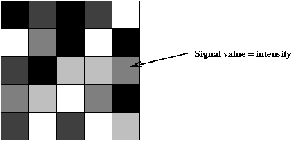
- Here is a 1D real-valued signal:
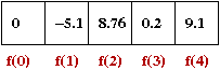
- We can treat each signal value as a greyscale intensity:
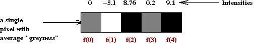
- Thus, a 2D array can be treated as a 2D array of intensities
→ an image!
- We'll assume square arrays of size \(N \times N\).
→ It's easy to generalize to \(M \times N\).
- Let's use the notation \(f(x,y)\) to denote the signal
value in cell \((x,y)\), where \(x\) and \(y\) are integers.
- Then, the input (signal) consists of:
- The number \(N\).
- A collection of \(N^2\) numbers \(f(x,y)\)
where \(0 \leq x \leq N-1\) and \(0 \leq y \leq N-1\).
- Alternatively, we can think of the input as
\(N^2\) complex numbers with the imaginary parts zero.
- The output (spectrum) will be a 2D array of complex numbers \(F(u,v)\).
- The two dimensional DFT is defined as:
$$
F(u,v) \eql \frac{1}{N^2}
\sum_{x,y} f(x,y) e^{-2\pi i(ux+vy)/N}
$$
- Likewise, the inverse DFT is defined as:
$$
f(x,y) \eql
\sum_{u,v} F(u,v) e^{2\pi i(ux+vy)/N}
$$
- The FFT can also be generalized analogously, but is rather more
complicated to describe.
In-Class Exercise 28:
Compile and execute DemoDFT2D.java.
You will also need Clickable2DGrid.java.
The top two grids represent the signal's real (left) and imaginary
(right) parts. The bottom two grids represent the spectrum.
- Select the middle grid cell in the spectrum's real components
and change this value to 100. Then, apply the inverse transform.
- Click on "showValues" to examine the signal's values.
- Change \(N\) to 20 and repeat. Experiment with setting only
one spectrum value to 100, but in different places.
The meaning of "frequency" in 2D:
- In 1D, frequency is a way of measuring how the signal fluctuates.
- In 2D, frequency measures fluctation of the signal spatially.
- Thus, a single spectrum value corresponds to a checkboard
pattern of some kind (depending on the frequency).
- Just like the 1D case, the signal is an addition of the
signals you get from individual frequencies.
What corresponds to removing high-frequencies in the 2D case?
- We can also remove high frequencies and produced a modified
signal image.
- This is the basis of lossy image compression.
- As it turns out, a DFT variant called the Discrete Cosine
Transform, is more commonly used in image compression.
10.8
Beyond linear combinations: some theory
For this section, we will return to the continuous
realm, functions, as opposed to discrete values.
Recall how we started describing Bernstein and trignometric
polynomials in the broader context of vectors:
- We expanded the notion of linear combination of vectors
to other mathematical objects:
$$
\alpha_1 \boxed{\color{white}{\text{LyL}}}_1
+ \alpha_2 \boxed{\color{white}{\text{LyL}}}_2
+ \ldots
+ \alpha_n \boxed{\color{white}{\text{LyL}}}_n
$$
- Using functions, we sought to study
linear combinations
$$
g(x) \eql \alpha_1 f_1(x) + \alpha_2 f_2(x) + \ldots +
\alpha_n f_n(x)
$$
- We saw that a linear combination of Bernstein polynomials
gave us a useful way to represent curves:
$$\eqb{
x(t) & \eql & a_0 (1-t)^3 + 3a_1 t (1-t)^2 + 3a_2 t^2(1-t) + a_3 t^3\\
y(t) & \eql & b_0 (1-t)^3 + 3b_1 t (1-t)^2 + 3b_2 t^2(1-t) + b_3 t^3
}$$
- Here, two different linear combinations were used, one each for the
\(x(t)\) and \(y(t)\) functions.
- By interpreting \((x(t), y(t))\) as a collection of points
on the plane, we get a Bezier curve, the foundation of
font design.
- By taking linear combinations of Bernstein-products, we
get Bezier surfaces, a workhorse of computer graphics.
- We also addressed some questions of theoretical interest:
- Are the Bernstein polynomials a basis for the space of
polynomials
Answer: yes
- Can a linear combination of Bernsteins approximate any
function closely?
Answer: yes
- But here's one we did not: are the Bernstein polynomials orthogonal?
Answer: sadly, no.
- It turns out, the Bernsteins can be tweaked to make them
orthogonal, and this has applications to other areas of mathematics
like differential equations.
- Let's now ask similar questions about the trig's:
- Are the trigonometric functions a basis of some kind?
- This is not a well-posed question, as it turns out.
- The reason is, we need to know: a basis for what?
- It's easy to categorize polynomials by their highest power.
- We could use the highest frequency as one possibility.
- In which case, the answer is: yes (but in a trivial way).
- For example, suppose
$$\eqb{
g(t) & \eql & 5 \sin(2\pi 3t) + 2 \sin(2\pi 8t) - \cos(\pi t)\\
}$$
This is already a linear combination of the basic sine's and cosine's.
- Can a linear combination of sine's and cosine's closely
approximate any function?
Answer: yes (this is Fourier's theorem)
- Are sine's and cosine's orthogonal?
Answer: yes!
Except that we have not described what it means for
two functions to be orthogonal.
- Recall the definition for vectors:
two vectors \({\bf u}\) and \({\bf v}\) are orthogonal
if
$$
{\bf u} \cdot {\bf v} \eql 0
$$
- With two functions \(f(t)\) and \(g(t)\), how do we define
orthogonality?
- Alternatively, how do we define a "dot" product (so that
orthogonal is the same as "dot product equals 0")?
- As a step towards definition, suppose \(f(t)\) and
\(g(t)\) are defined over some interval like \([0,1]\).
- Now divide \([0,1]\) into many (\(m\)) equal-sized small
intervals:
- That is, define numbers \(t_1=0, t_2, t_3, \ldots, t_m=1\)
where \(t_1 < t_2 < t_3 < \ldots < t_m\).
- The smaller intervals are \([t_1,t_2], [t_2,t_3], \ldots, [t_{m-1},t_m]\).
- Consider the function's values at these various "ticks"
between \([0,1]\):
- \(f(t_1), f(t_2), f(t_3), \ldots, f(t_m)\) are the f-function
values.
- \(g(t_1), g(t_2), g(t_3), \ldots, g(t_m)\) are the g-function
values.
- Let's treat these values as components of an m-element vector:
- The vector \({\bf f} = (f(t_1), f(t_2), \ldots, f(t_m))\).
- The vector \({\bf g} = (g(t_1), g(t_2), \ldots, g(t_m))\).
- Then the dot-product of the two vectors turns out to be:
$$\eqb{
{\bf f} \cdot {\bf g} & \eql &
f(t_1)g(t_1) + f(t_2)g(t_2) + \ldots + f(t_m)g(t_m) \\
& \eql & \sum_{i=1}^m f(t_i) g(t_i)
}$$
We could use this as an "approximate" dot-product for two functions.
- Now suppose \(\delta = (t_{k+1}-t_k)\), the length of an interval.
- We can scale the approximate dot-product so that it's
$$\eqb{
\delta \;\; ({\bf f} \cdot {\bf g}) & \eql &
\sum_{i=1}^m f(t_i) g(t_i)\delta
}$$
- Now you can see where we're going with this. In the limit
as \(m\) gets large (for better and better accuracy),
we are led to the definition
$$
f \cdot g \eql \int_0^1 f(t)g(t) dt
$$
- In general, for any arbitrary interval, we define the
dot-product of two functions \(f\) and \(g\) as
$$
f \cdot g \eql \int_0^\infty f(t)g(t) dt
$$
- Luckily,
this turns out to be easy to compute for sine's and cosine's.
- From which one can show that sine's and cosine's are
orthogonal. For example:
$$
\sin(2\pi t) \cdot \sin(2\pi 2t)
\eql \int_0^{2\pi} \sin(2\pi t) \sin(2\pi 2t) dt
\eql 0
$$
Why do we care that they are orthogonal?
- Orthogonality makes calculations a lot easier than if we didn't
have an orthogonal basis.
- Orthogonality makes proofs (for theory) easier.
- It turns out that there are other orthogonal collections
of basis functions, like Legendre polynomials.
- There is a rich mathematical theory of such functions and
their uses, which we won't explore here.
© 2016, Rahul Simha