Module objectives
The goal of this module is to:
- Review some basic ideas about numbers, and the different
types of numbers.
- Introduce complex numbers.
- Review basic facts about polynomials.
- Review 1D and 2D arrays.
2.0
Meet the integers
About integers:
- We usually include both positive and negative
integers
\(\mathbb{Z} = \{\ldots, -3, -2, -1, 0, 1, 2, 3, \dots\} \)
- Note: \( \mathbb{N} = \{1, 2, 3, \ldots\} \)
are the natural numbers.
\(\rhd\)
(Some people include \(0\)).
- In many problems, we might only consider particular
(finite or infinite) subsets of \(\mathbb{Z}\)
- Things we do with integers:
- Standard arithmetic operators that result in integers:
\( +, -, \times \)
\(\rhd\)
Integer division needed for an integer result
- Use operators to define special classes of integers, e.g., primes,
\(\rhd\)
Then prove interesting, and occasionally useful (e.g., crypto), results.
- Did you know \(70\) is the smallest weird number?
- Some famous problems/results:
- The Fundamental Theorem of Arithmetic: Every integer larger
than 1 is either a prime or a unique product of primes.
- (Solved in 1995) Fermat's Last Theorem: There are no integers
\(x,y,z\) such that \(x^n + y^n = z^n\)
for every integer n > 2.
- (Unsolved) Goldbach's conjecture (1742): Every even
integer greater than 2 can be written as the sum of two primes.
- (Unsolved) Polynomial-time algorithm for factorizing an integer.
In-Class Exercise 1:
Prove that the square root of an even square number is even.
2.1
Meet the rationals
About the rationals:
- We know that \(3 \div 2 = 1\) using integer division.
- Yet, if treated as a length, we know that something
of length 3 can actually be divided into two equal pieces.
- The length of one of those pieces is not an integer length
\(\rhd\)
We'd like such lengths or measurements to be numbers.
- A simple idea for a definition: use division
\(\rhd\)
A rational number is the length you get
when an integer \(p\) divided into \(q\) equal pieces.
- More formally: the ratio \(\frac{p}{q}\) where
\(p\) and \(q\) are integers.
- The rational numbers \(\frac{2}{4}\) or \(\frac{30}{60}\) are the same
as \(\frac{1}{2}\)
\(\rhd\)
We use the "most simplified" form \(\frac{1}{2}\)
- Simplified form: the ratio \(\frac{p}{q}\) where
\(p\) and \(q\) are integers with no common divisors other than 1.
- Commonly used symbol:
\(\mathbb{Q} = \) the set of rational numbers.
- What's nice: the usual operators \(+,-,\times,\div\) all
result in rational numbers.
In-Class Exercise 2:
Prove or disprove: given any two rational numbers \(x\) and
\(y\) such that \(x < y \) there is at least one rational
number \(z\) in between: \(x < z < y\).
A problem with rational numbers:
- Consider the square-root operation: \(\sqrt{x}\) for
a rational number \(x\).
- A question: is \(\sqrt{x}\) always rational?
- Example: \(\sqrt{2}\)
In-Class Exercise 3:
Is there a real-world physical length corresponding to
\(\sqrt{2}\)?
Let's dive into our first proof:
Proposition 2.1
\(\sqrt{2}\) is not rational.
Proof
So, there are numbers that are irrational.
A burning question: are there other types of numbers?
That is, if we combine the rationals and the irrationals, do we
get all possible numbers?
2.2
Meet the reals
About the reals:
- Standard notation: \(\mathbb{R}\)
- Loosely, the reals are the union of the rationals and irrationals.
- But this raises the question: is there a "length" that would
be non-real?
- As it turns out, this is not a simple question
\(\rhd\)
It took years for mathematicians to carefully define real numbers.
- The definition is complicated, and uses a bunch of rules
about operators, ordering etc.
- One interesting and powerful result: the real number
system is unique.
\(\rhd\)
Any two number systems satisfying those axioms are equivalent.
- Informally, we think of real numbers as "possibly having digits after
the decimal point."
- Examples: 3.141, 2.718.
- Given any two real numbers, there is another real between them.
- So far, we haven't asked how "rare" irrationals are.
- It appears that rationals "fill up" the number line.
- All we know about irrationals: some particular numbers are irrational.
A problem with reals:
- We can write \(x=\sqrt{2}\) as the solution to the equation
\(x^2-2 = 0\).
- In general, it's of great interest to solve equations
like
\(a_nx^n + a_{n-1}x^{n-1} + \ldots + a_1x_1 + a_0 = 0\)
- One question: is it true that any solution must be a real number?
- What about the solution to \(x^2 + 2 = 0\)?
- We will get to this issue later.
Algebraics and transcendentals
- An algebraic real number is a real number that is the solution
to some polynomial equation with integer coefficients.
- Thus, for \(x\) to be an algebraic number, \(x\)
there need to be integers \(a_0,\ldots,a_n\) such that
\(a_nx^n + a_{n-1}x^{n-1} + \ldots + a_1x_1 + a_0 = 0\)
- A number that is not algebraic is called transcendental.
In-Class Exercise 4:
- Explain why, if we changed the definition above so that
the coefficients \(a_i\) are rational (instead of integers),
we'd get the same set of algebraic numbers as we get with
integer coefficients.
- Are there non-rational algebraic numbers?
A famous algebraic number: \(\phi\)
- The equation \(x^2 - x - 1 = 0\) has two solutions, one
of which is \(\phi = \frac{1+\sqrt{5}}{2} \approx 1.6180339...\).
- Often called the golden ratio.
\(\rhd\)
One of the most fascinating and studied numbers in history
- Shows up in nature, geometry, Fibonacci series, other examples.
Transcendentals:
- Many well-known numbers like \(\pi\) and \(e\) are
transcendental.
- It is generally not easy to prove that a number is
transcendental.
Clearly, there are lots of algebraic numbers (lots of
polynomials).
But it's not (yet) clear how many transcendentals there are.
2.3
Countability
For finite sets, the size of the set is the number of elements.
For infinite sets, it's a little more complicated:
Two infinite sets A and B have the same cardinality
if there is a 1-1 mapping between their elements.
Example: \(\mathbb{Z}\) and \(\mathbb{N}\):
$$\eqb{
1 \;\;\; & \;\;\; 0 \\
2 \;\;\; & \;\;\; 1 \\
3 \;\;\; & \;\;\; -1 \\
4 \;\;\; & \;\;\; 2 \\
5 \;\;\; & \;\;\; -2 \\
6 \;\;\; & \;\;\; 3 \\
7 \;\;\; & \;\;\; -3 \\
...
}$$
In-Class Exercise 5:
What is the 1-1 function that takes an integer and produces
the corresponding natural number?
In-Class Exercise 6:
What about the size of the rationals compared to integers?
The size of the reals is much larger than that of naturals:
(Proofsketch)
- Suppose that integers and reals had the same size.
⇒
Then, there is a 1-1 mapping
⇒
Then, one could list the reals according to this mapping
1. \(r_1\)
2. \(r_2\)
3. \(r_3\)
....
- Consider the real s constructed as follows:
the i-th digit of s differs from the i-th
digit of ri.
- Then, s is not in the list.
⇒
A contradiction!
- Terminology:
- The integers and other infinite sets of the same cardinality
are called countable.
- The reals are uncountable.
Note:
- The above proof was Cantor's second proof.
- His first proof showed the algebraic numbers are countable
⇒
Transcendentals are uncountable
- Cantor did not acknowledge Richard Dedekind's contribution
(first person to sort out the earlier issue of defining real numbers).
- The cardinality of any real interval \([a,b] \subset \mathbb{R}\)
is the same as that of \(\mathbb{R}\).
In-Class Exercise 7:
Show that the cardinality of
\([0,1]\) is the same as that of any \([a,b]\), for example
\([0,10]\).
A related idea: density
- The rationals are dense among the reals: given any real number
\(x\) and any arbitrarily small number \(\epsilon\), there is
a rational between \(x\) and \(x+\epsilon\).
- The integers are not dense among the reals.
Other types of "numbers"
- An interesting question: is there a set who's countability (size) is between the integers and the reals?
\(\rhd\)
Not known
- The symbol \(\aleph_0\) is used to describe the size (cardinality)
of the integers.
- \(\aleph_1\) is the "next" infinite size.
- The cardinalities \(\aleph_0, \aleph_1,...\) can be
conceptually treated as "numbers"
\(\rhd\)
Called the transfinite numbers.
- One can define abstract rules of arithmetic for transfinite numbers.
\(\rhd\)
Quite esoteric
2.4
Functions and coordinates
What is a function?
- Intuitively, a function is something that "computes" a result
given an input.
- For example, \(f(x) = x^2\) takes a number \(x\) and
produces its square.
- Alternatively, we can think of a function as an association:
the square function associates every number with its
square, e.g.,
$$
\begin{array}{lll}
2
\;\;\;\;\; & \;\;\;\;\;
\mbox{is associated with}
\;\;\;\;\; & \;\;\;\;\;
4\\
3
\;\;\;\;\; & \;\;\;\;\;
\mbox{is associated with}
\;\;\;\;\; & \;\;\;\;\;
9\\
3.126
\;\;\;\;\; & \;\;\;\;\;
\mbox{is associated with}
\;\;\;\;\; & \;\;\;\;\;
9.771876\\
\end{array}
$$
Here, there is no specified computation.
The "association" view becomes useful when we consider coordinates
Early (Greek) geometry developed entirely without coordinates.
- Thought to have originated with Thales.
- Example:
Proposition 2.2: An inscribed triangle with the diameter as a side is a
right-angled triangle.
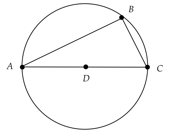
Proof: Draw the line segment \(BD\).
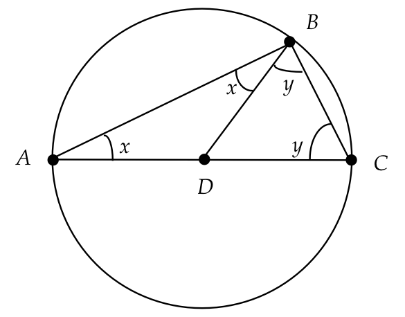
Because \(AD=DB, \bigtriangleup ADB\) is isoceles and so
\(\angle DAB = \angle ABD\). Similarly,
\(\angle DBC = \angle BCD\). Thus, adding up the angles
of \(\bigtriangleup ABC\), \(x+y+(x+y)=180^\circ\)
or \(x+y=90^\circ\), which is \(\angle ABC\).
- The converse is also true: there is only one circle
that circumsribes a right-angled triangle and its diameter
is the hypotenuse.
Proof: interestingly, we will use linear algebra to
prove this (later).
- A great deal of early geometry had no "numbers"
\(\rhd\)
Most often, reasoning was about relationships between angles and lengths
- Later geometry did feature numeric quantities:
areas and volumes.
- Many sophisticated results: geometrical constructions,
proofs of properties, conics, areas and volumes.
\(\rhd\)
Example: trisecting a
line segment (not trivial)
- But they got "stuck" with some problems, e.g., angle
trisection with only ruler and compass.
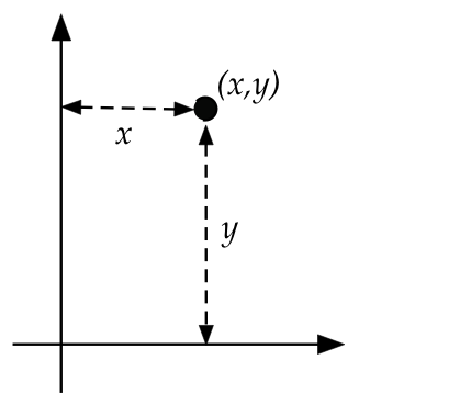
Enter Descartes ("I think, therefore I need coordinates")
- With an astonishingly simple idea: associate two numbers with
every point in the plane
\(\rhd\)
distances from two fixed lines (called axes)
- Which allowed algebraic representations of geometric ideas
\(\rhd\)
lines, curves, surfaces, area, volumes
- Eventually, the angle trisection problem was resolved
through algebra
\(\rhd\)
Shown to be impossible, in general
- Coordinates also led to an appealing visualization of
functions:
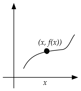
- Descartes introduced the modern convention for notating
basic algebra, such as variables (\(x,y,z\)), exponentiation (\(x^y\))
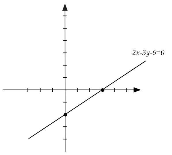
More about points and lines:
In-Class Exercise 9:
Why is \(ax+by+c=0\) the equation of a line? Can you find
an argument using simple geometry (similar triangles)?
More about functions:
- The general idea of and notation for single-variable
functions is easily extended to:
- Multiple variables, e.g. \(f(x,y,z)\)
- Function composition, e.g., \(f(g(x))\)
- An inverse of a function, \(f^{-1}(x)\)
- One can characterize the behavior of functions abstractly:
\(\rhd\)
continuous functions, differentiable functions etc.
- Notation: \(C[a,b] = \) the set of continuous functions
on the interval \([a,b]\).
In-Class Exercise 10:
Consider the two-variable function
\(f(x,y) = (x+y)^n\). Show that
\((x+y)^n = \sum_{k=0}^n \nchoose{n}{k} x^k y^{n-k}\)
2.5
Polynomials
Polynomials are a special category of functions
- Definition: A (single-variable) polynomial is a function
with the following form:
$$f(x) = a_nx^n + a_{n-1}x^{n-1} + \ldots + a_1x_1 + a_0$$
where the coefficients \(a_i\) are real numbers.
For example
$$ f(x) = x^2 - x - 1$$
- The degree is the highest power.
- Polynomials were historically important because they were
among the first equations to be solved, e.g., quadratics, cubics etc.
An interesting question: are the types of curves representable
by polynomials a small set?
- One important result: Taylor's Theorem
Any function that can be successively
differentiated \(k\) times can be approximated closely near a point
by a degree-\(k\) polynomial at that point
$$
f(x) \;\;\; \approx \;\;\;
f(a) + f'(a)(x-a) + \frac{f''(a)}{2!}(x-a)^2 + \ldots
\frac{f^{(k)}(a)}{k!} (x-a)^k
$$
- One limitation: the polynomial is different at different points.
- Later, a major result: the Stone-Weierstrass theorem:
Any continuous function can be approximated arbitrarily
closely by a polynomial.
- Alternatively: polynomials are dense in the set of
of continuous functions.
Another observation:
- Consider these particular polynomials:
\(p_0(x) = 1\), a constant polynomial
\(p_1(x) = x\)
\(p_2(x) = x^2\)
\(p_3(x) = x^3\)
...
\(p_k(x) = x^k\)
- Any polynomial \(p(x)\) is a linear combination of the
above polynomials:
$$\eqb{
p(x) & \;\; = \;\; & a_nx^n + a_{n-1}x^{n-1} + \ldots + a_1x_1 + a_0\\
& \;\; = \;\; & a_np_n(x) + a_{n-1}p_{n-1}(x) + \ldots + a_1p_1(x) + a_0p_0(x)
}$$
- This will turn out to be an important idea in linear algebra.
- Thus, by Stone-Weierstrass, any continuous function
can be represented by a linear combination of these basic powers.
A special kind of polynomial: Bernstein polynomial
Taylor series:
- Recall: Any function that can be successively
differentiated \(k\) times can be approximated closely near a point
by a degree-\(k\) polynomial at that point
$$
f(x) \;\;\; \approx \;\;\;
f(a) + f'(a)(x-a) + \frac{f''(a)}{2!}(x-a)^2 + \ldots
\frac{f^{(k)}(a)}{k!} (x-a)^k
$$
- For a function that can be infinitely differentiated,
(\(f^{(k)}(x)\) exists for all \(k\)), one wonders if
$$
f(x) \;\;\; = \;\;\;
f(a) + f'(a)(x-a) + \frac{f''(a)}{2!}(x-a)^2 + \ldots
\mbox{ (infinite sum)?}
$$
- Turns out that it is exact for many important
functions, e.g.,
$$\eqb{
e^x & \;\; = \;\; & 1 + x + \frac{x^2}{2!} + \frac{x^3}{3!}
+ \ldots \\
\sin(x) & \;\; = \;\; & x - \frac{x^3}{3!} + \frac{x^5}{5!}
- \frac{x^7}{7!} + \ldots \\
\cos(x) & \;\; = \;\; & 1 - \frac{x^2}{2!} + \frac{x^4}{4!}
- \frac{x^6}{6!} + \ldots \\
}$$
- The above three series turn out of have great significance:
- One is practical: they give an algorithm for
computing these functions.
- The other is theoretical, in the case of complex numbers (below).
2.6
Trigonometric functions
Aside from polynomials, the "trigs" are perhaps the most
important class of functions. Let's review.
- What are \(\sin\) and \(\cos\)?
- We often think: \(\sin(\theta)\) = ratio of opposite side
to hypotenuse when the angle is \(\theta\).
- A better way: think of it as a function:
\(\rhd\)
For a variable \(\theta\),
the function \(\sin(\theta)\) is well-defined.
- Convention: measure angle in radians where a radian is
defined such that \(2\pi\) radians = 360o.
- Important: \(\sin(\theta)\) is defined for all
\(-\infty < \theta < \infty\).
In-Class Exercise 12:
Let's explore the last point.
- Note: \(2\pi\) is approximately \(6.29\).
Why is it OK to define a value for \(\sin(17.5)\)
or \(\sin(-156.32)\)? How are these values defined?
- Download PlotSin.java,
Function.java,
and
SimplePlotPanel.java.
Then compile and execute PlotSin.java
to plot the function sin and cos in the range [0,20].
How many times does the function "repeat" in this range?
Next, let's understand the concept of frequency:
- In English: it refers to "how often"
\(\rhd\)
There is an implied notion of time.
- For a sinusoid like \(\sin(t)\), it means "how often the
function repeats itself per unit time".
- To understand this better, let's see what a cycle means:
- Since \(\sin(t + 2\pi) = \sin(t)\),
the crest-and-trough shape repeats.
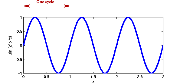
- A single crest-and-trough is called a cycle.
- The frequency is the number of cycles per unit time.
\(\rhd\)
The unit of measurement is called a Hz (Hertz), the number
of cycles per unit time.
- Let's examine the function \(\sin(2\pi\omega t)\).
In-Class Exercise 13:
Compile and execute PlotSin2.java
to plot \(\sin(2\pi\omega t)\)
in the range \([0,1]\) with \(\omega = 1, 2, 3\).
What is the relationship between the three curves?
- Thus, \(\omega\) is the frequency: the number of cycles
per second.
- Note: \(\omega\) can be a real number.
\(\rhd\)
You can have a frequency of 3.356 cycles per second.
- The function \(\sin(2\pi k\omega t)\), for integer
\(k\), is called a harmonic of \(\sin(2\pi \omega t)\)
\(\rhd\)
\(k\) cycles of \(\sin(2\pi k\omega t)\) fit into one
single cycle of \(\sin(2\pi \omega t)\)
- The inverse of frequency is called the period, the
length of time for one complete cycle.
- You can shift a sin wave by adding a fixed constant to the
argument: \(\sin(2\pi\omega t + \phi)\)
In-Class Exercise 14:
Modify PlotSin3.java to plot
\(\sin(2\pi t + \phi)\) in the range \([0,1]\). Plot four
separate curves with \(\phi=0, \frac{\pi}{4}, \frac{\pi}{2}, \pi\).
What can you say about \(\sin(2\pi t + \frac{\pi}{2})\)?
Similarly, plot \(\cos(2\pi t + \frac{\pi}{2})\)
and comment on the function.
Finally, the third parameter to a sinusoid is its amplitude:
Trigonometric "polynomials"
- Just like \(x^n\) is a "basic" polynomial, one can
consider \(\sin(n x)\) and \(\cos(nx)\) to be
"basic" sin/cos building blocks.
\(\rhd\)
Sometimes called the trigonmetric polynomials
- It turns out that the trig polynomials are
dense in the space of continuous functions
\(\rhd\)
This the celebrated Fourier theorem:
$$
f(t) \;\; = \;\;
a_0 + \sum_{k=1}^\infty a_k \sin(2\pi kt/T)
+ \sum_{k=1}^\infty b_k \cos(2\pi kt/T)
$$
for any continuous function \(f(t)\) over an interval \([0,T]\).
- Thus, a linear combination of the basic trig's can
be used to approximate a function as closely as desired.
- As it turns out, the calculation of the constants
\(a_i, b_i\) arises from linear algebra.
2.7
Complex numbers
What are they and where did they come from?
Conjugates:
- It turns out to be really useful to define something called
a conjugate of a complex number \(z = a+ib\):
$$\eqb{
\overline{z} \;\; = \;\; \overline{a + ib} \\
\;\; \defn \;\; a - ib
}$$
- The magnitude of a complex number \(z = a+ib\) is
the real number
$$
|z| \;\; \defn \;\; \sqrt{a^2 + b^2} \;\; = \;\; \sqrt{z\overline{z}}
$$
The magnitude will have meaning below once we
associate a geometrical interpretation
to complex numbers: the distance from the origin to
the point representing \(z\).
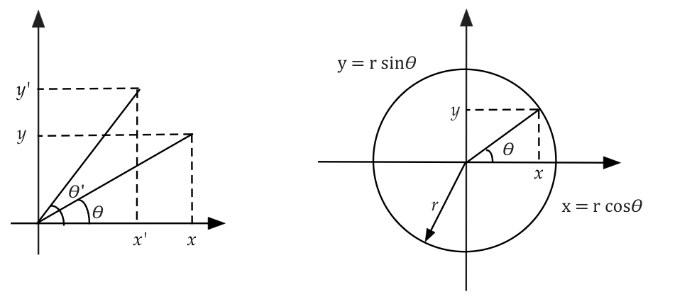
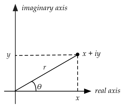
Polar representation of complex numbers:
- One useful graphical representation is obvious when we write
complex number \(z\) as \(z = x + iy\).
- Given this, one can easily write
$$\eqb{
z & \;\; = \;\; & x + i y \\
& = & r\cos(\theta) + i r \sin(\theta) \\
& = & r \left( \cos(\theta) + i \sin(\theta) \right) \\
}
$$
- An important observation made by Euler:
Suppose you define
$$
e^z \;\; \defn \;\;
1 + z + \frac{z^2}{2!} + \frac{z^3}{3!} + \ldots
\mbox{ (analogous to the Taylor series for the real function \(e^x\))}
$$
Then
$$\eqb{
e^{i\theta} & \;\; = \;\; &
1 + i\theta + \frac{(i\theta)^2}{2!} + \frac{(i\theta)^3}{3!} + \ldots
\\
& \;\; = \;\; &
\mbox{(series for \(\cos(\theta)\))} +
i \mbox{ (series for \(\sin(\theta)\)) } \\
& \;\; = \;\; &
\cos(\theta) + i \sin(\theta)
}
$$
This is called Euler's relation.
- More generally, \(re^{i\theta} = r(\cos(\theta) + i \sin(\theta))\)
- Think of \(z = re^{i\theta}\) as the polar
representation of the complex number
\(z = x+iy = r(cos(\theta) + i \sin(\theta))\).
Roots of 1:
Observe: when \(r=1\), and \(\theta=2\pi\)
or \(\theta= - 2\pi\)
- \(e^{2\pi i} = 1\) and \(e^{-2\pi i} = 1\)
- Next, \( (e^{2\pi i/N})^N = 1\)
and \( (e^{-2\pi i/N})^N = 1\), for any \(N\).
In particular, this means that \(e^{2\pi i/N}\)
and \(e^{-2\pi i/N}\) are \(N^{th}\) roots of \(1\).
We will use the notation
$$\eqb{
W_N & \;\;= \;\; & e^{2\pi i/N} \\
W_N^* & \;\;= \;\; & e^{-2\pi i/N} \\
}$$
Lastly, because \(\cos(-x)=\cos(x)\) and \(\sin(-x)=-sin(x)\).
$$
e^{-2\pi i/N}
\;\; = \;\; \cos(\frac{2\pi}{N}) - i \sin(\frac{2\pi}{N})
$$
To summarize:
$$\eqb{
W_N & \;\; = \;\; & e^{2\pi i/N} & \;\; = \;\; &
\cos(\frac{2\pi}{N}) + i \sin(\frac{2\pi}{N}) \\
W_N^* & \;\; = \;\; & e^{-2\pi i/N} & \;\; = \;\; &
\cos(\frac{2\pi}{N}) - i \sin(\frac{2\pi}{N}) \\
}$$
An aside: powers of \(W_N\) give us the other N-th roots:
$$
(W_N^k)^N \; = \; (W_N^N)^k \; = \; (1)^k \; = \; 1
$$
Thus, \(W_N^0, W_N^1, W_N^2, \ldots, W_N^{N-1}\)
are the \(N\) N-th roots of unity.
Implementing complex numbers:
- One can use a simple object to represent a complex number, for example:
public class Complex {

    // Real and imaginary parts
    double re, im;

    public Complex (double re, double im)
    {
        this.re = re;
        this.im = im;
    }

    public Complex add (Complex c)
    {
        return new Complex (re + c.re, im + c.im);
    }

    public Complex mult (Complex c)
    {
        return new Complex (re*c.re - im*c.im, re*c.im + im*c.re);
    }

}
- With this, we can write code like:
        // Make one complex number (recognize this one?):
        Complex c1 = new Complex (Math.cos(2*Math.PI/N), -Math.sin(2*Math.PI/N));

        // Make another:
        Complex c2 = new Complex (1, 0);

        // Multiply:
        Complex result = c1.mult (c2);
2.8
Arrays
Consider a simple one dimensional array
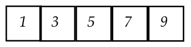
Some sample code to create and populate this array:
(source code)
	int n = 5;                      // Array size.
	int[] A = new int [n];          // Create the space.
	for (int k=0; k<n; k++) {
	    A[k] = 2*k + 1;             // Populate the array.
	}
And an example of doing something with the array's contents:
	int[] B = new int [n];
	B[0] = A[0];
	for (int k=1; k<n; k++) {
	    B[k] = B[k-1] + A[k];
	}
Can you see what the array B will contain?
In-Class Exercise 17:
As a little practice exercise with one dimensional arrays,
write some code to determine whether a string is a
double-palindrome. Download
ArrayExamples.java,
which explains what a double-palindrome is, and write your
code in Palindrome.java.
Two dimensional arrays:

- The above is an example of a \(4 \times 6\) array: 4 rows, 6 columns.
- Here is some sample code:
	double[][] A = new double [4][6];
	A[1][4] = 0.5;
- Both 1D and 2D arrays will be a staple of this course:
vectors will be 1D and matrices will be 2D.
Images:
- First, let's understand what a greyscale image is:
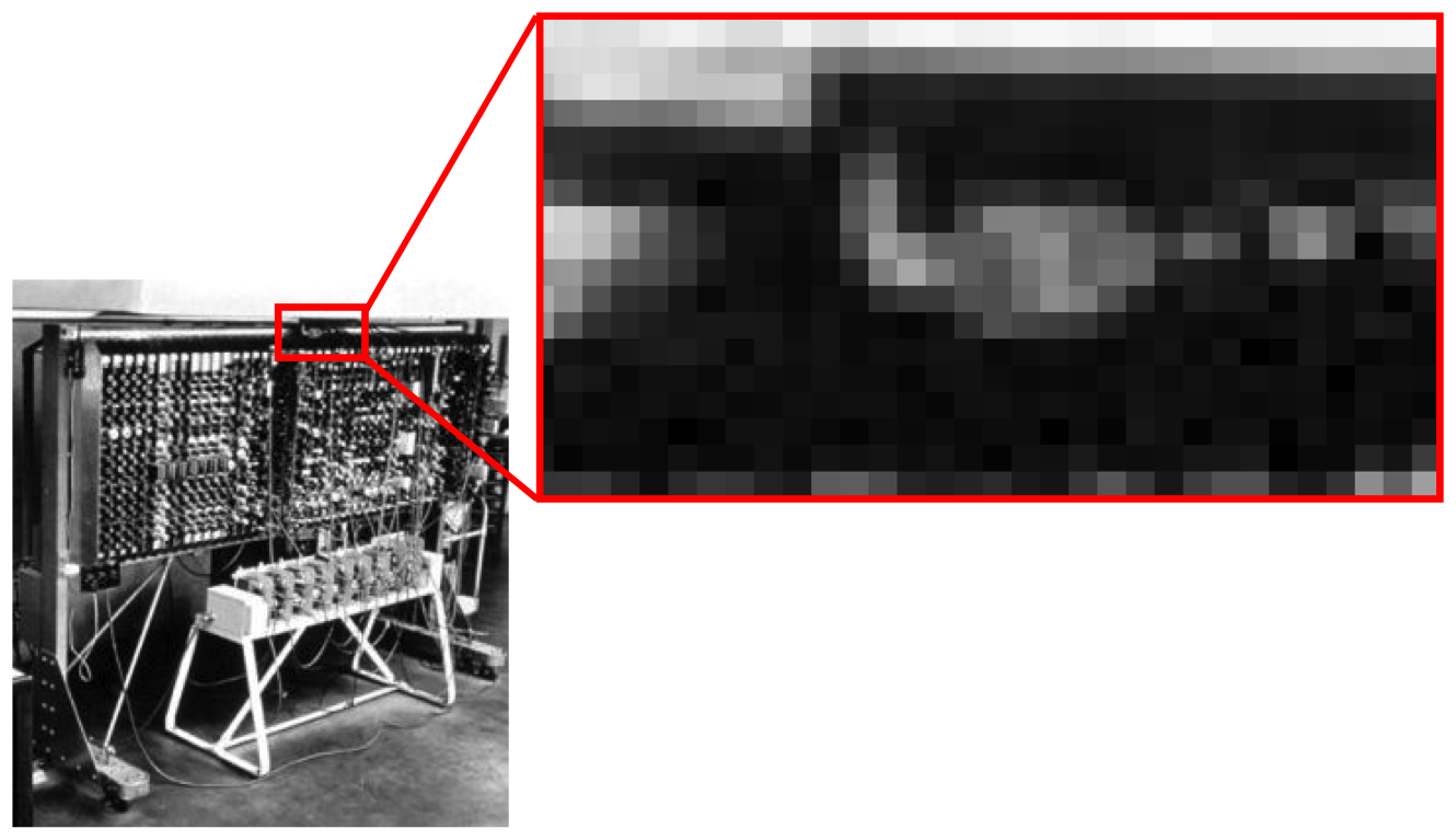
- A (greyscale) image is really a 2D array of "grey" intensities.
- Commonly, the intensity is a number between 0 and 255.
- Here is some code that reads a JPG image and converts into
pixels:
	ImageTool imTool = new ImageTool ();
	int[][] pixels = imTool.imageFileToGreyPixels ("ace.jpg");
In-Class Exercise 18:
Write code to blur an image. Start by
writing pseudocode to solve the problem.
Then, download
ImageBlur.java,
which contains instructions, and where you will write your
code. You will also need
ImageTool.java.
And as a test image, you can use ace.jpg.
In-Class Exercise 19:
Let's examine the idea of computing the "distance" between
two arrays.
- A distance measure should take two arrays and return
a non-negative number.
- Propose a "distance" calculation for 1D arrays.
- Propose an extension of that idea to 2D arrays.
Do the arrays have to be of the same length?
In-Class Exercise 20:
How is a 2D array stored in memory? Consider this code snippet:
	double[][] A = new double [4][6];
	A[1][4] = 0.5;
	double[][] B = A;
	B[1][4] = 0;
	System.out.println (A[1][4]);       // What gets printed out?
What does it mean to make a "deep copy" of an array?
OK, we're now ready to tackle linear algebra.
2.9
Highlights and study tips
Highlights of this module:
- There are different types of numbers (integers, rationals,
reals, complex numbers).
- The sizes of these sets are different (countable, uncountable).
- Polynomials are an important class of functions
- They're easy to work with.
- Dense in the space of functions (Stone-Weierstrass, Bernstein).
- Polynomial series (Taylor series) are useful both
computationally (e.g., to compute \(\sin(x)\)) and
theoretically (to define \(\sin(z)\) for complex \(z\)).
- The "trigs" are an equally important class of functions,
also dense among functions (Fourier's theorem).
- We'll see that the trigs play a key role in signal processing.
- Complex numbers are ...
- a bit weird, with specialized arithmetic and function definitions;
- an extremely important development that "completes" the solution
of polynomial equations;
- unexpectedly useful in some applications like signal processing.
- Arrays are the backbone of scientific code, especially 1D
and 2D arrays that are the workhorses of linear algebra.
Some general suggestions about how best to learn:
- Do not delay completing the in-class exercises.
- The worst way to learn mathematical ideas is to read and then
not follow up.
- Instead, after reading, it's best to "do" something: either
work on some problems or write out the same ideas in your voice.
- Keep a notebook and write notes:
- Don't write mindlessly. Think as you write.
- This way, if anything needs elaboration you should add that.
- If you've acquired a textbook, read the text after
your notes so that you can read at a deeper level.
- For proofs:
- It can help to work through an example along with the
proof. (This works best for proofs that grind through algebra.)
- Leave no stone unturned regarding proofs:
That is, if there's a proof detail that's unclear, try
to address it.
- You've really understood a proof if you can replicate it without
notes or help, and can explain it.
This module was a whirlwind tour through some basic ideas in
mathematics.
- Not every detail is really needed per se for the
rest of the course.
- The in-class exercises, however, are good practice
for mathematical thinking.
- The array practice exercises are worth doing right away.