Determining the readability and reading-level of a passage
is critical in helping teachers select text passages in grade school.
We'll use the F-K reading ease score
$$
206.835 - 1.015 \left(\frac{\mbox{total words}}{\mbox{total sentences}}\right)
-84.6 \left(\frac{\mbox{total syllables}}{\mbox{total words}}\right)
$$
Thus, for a passage, we need to count the total number of words,
the total number of sentences and the total number of syllables.
The result will be a number no higher than 121.22.
Here are example ranges:
  > 100:      4th grade and below, simple words
  90 - 100:   5th grade
  50 - 60:    10th-12th grade
   0 - 10:    Professional
For example, "Bill had a bat and a ball" has an F-K score of
-35.78.
And this typical example from contract law (cited
the Harvard
Business Review) has a score of 4.95
Under no circumstances shall company have any liability,
whether in contract, tort (including negligence), strict
liability, other legal theory, or breach of warranty for:
any lost profits; any loss or replacement of data files lost
or damaged; consequential, special, punitive, incidental, or
indirect damages arising out of this agreement, the delivery,
use, support, operation, or failure of the system; or consequential,
special, punitive, incidental or indirect damages arising out
of the inaccuracy or loss of any data generated by the system;
even if company has been advised of the possibility of such
damages, provide that the foregoing disclaimer
under sub-section (iii) above does not apply to the extent
such damages are based upon the use of the system and are
arising out of willful misconduct or gross negligence that results
in a breach of section 6 hereto.
In case you're wondering how they came up with this weird formula:
This is an example of what statisticians called
linear regression.
One starts with text samples that are scored by experts (by hand).
Then, one decides what variables to use. In this case:
$$\eqb{
x_1 & = & \left(\frac{\mbox{total words}}{\mbox{total sentences}}\right)\\
x_2 & = & \left(\frac{\mbox{total syllables}}{\mbox{total words}}\right)
}$$
The values of these variables are known for the text samples.
Then, one solves
$$
\alpha + \beta x_1 + \gamma x_2 = s
$$
across the collection of scored texts.
With real data, equations can give you weird solutions.
Now let's consider automated scoring:
The easy part is counting words and sentences: wordtool already
has that feature:
sentence_count = 0
word_count = 0

s = wt.next_sentence_as_list()

while s != None:
    sentence_count += 1
    word_count += len(s)
    for w in s:
        # This is where we'd like the syllable count for word w

    s = wt.next_sentence_as_list()

# After the loop we'll have word_count and sentence_count.
Let's focus on counting syllables:
while s != None:
    sentence_count += 1
    word_count += len(s)
    for w in s:
        # This is where we'd like the syllable count for word w
        syllable_count += syllable.count_syllables(w)

    s = wt.next_sentence_as_list()
Here, we're going to write a function called
count_syllables()
in another file called
syllable.py.
Thus
syllable.py.
will look something like:
def count_syllables(w):
    count = 0

    # ... the code for determining the number of syllables in w ...

    return count
The rules we will use are:
Treat 'y' as a vowel
If the first letter is a vowel increment by 1.
For the remaining letters,
if a letter is a vowel and the previous one is not,
count that as a syllable.
If the word ends with 'e', decrease the count, but only if
the letter to its left is not a vowel
Ensure that the syllable count is at least 1.
Of course, these rules aren't perfect. They will not
catch every single syllable but will be good enough for scoring text.
3.21 Exercise:
Download the following:
syllable.py
and
test_syllable.py.
Then fill in code to implement the syllable counting
rules and run the tests in
test_syllable.py.
In your module pdf, report on the FK-score for each of these.
Analyze a text from Project Gutenberg (or elsewhere)
whose FK score is surprising (either unexpectedly low or unexpectedly
high), and explain why it's surprising.
Part B: Word-cloud analysis of text
What we'd like to do in this part is to run an analysis of text
and produce a quick telling snapshot of the whole text.
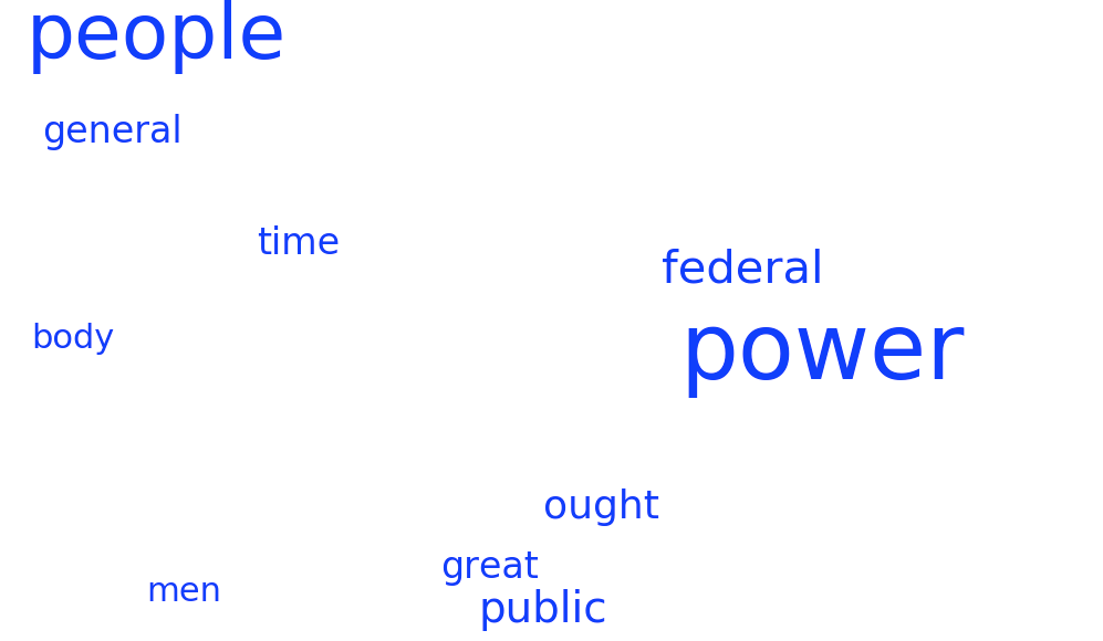
For example, here's a word-cloud of the 10 most frequently
occuring words in the Federalist Papers:
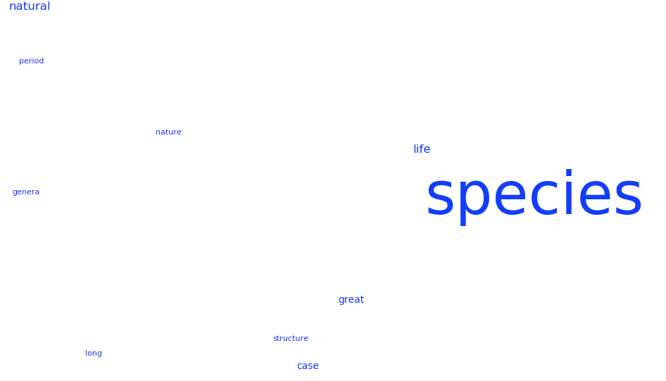
And for comparison, the same for Darwin's Origin of the Species:
If you only looked at the snapshot and hadn't been told
the book titles, surely you could say the first one was about
government or politics, and the second about biology.
Of course there are now far more sophisticated ways of
automatically analyzing text. But a good starting point
is a simple word cloud:
We'll count the occurence of nouns (to simplify) in a text.
Then we'll identify the 10 most frequently occuring nouns.
After that, we'll draw using font sizes proportional to occurrence.
Later, you'll improve on the drawing (you can see that
"species" practically hides all the other nouns in Darwin's cloud).
Let's start with counting nouns:
First, it's a good idea to review both
tuples and dictionaries
from Module 1.
We'll use wordtool to read a file word-by-word, and
wordtool also has a list of nouns, which will let us check whether
a word is a noun.
We'll be careful to avoid so-called stopwords:
These are common short words like "a", "an", "the".
While most aren't nouns, we'll nonetheless remove them
because any kind of word analysis typically begins by removing
stopwords.
So, the general idea in counting nouns is:
import wordtool as wt

nouns = wt.get_nouns()              # Wordtool will build this list
stop_words = wt.get_stop_words()    # And this one.

# We'll use this dictionary for counting occurrence:
noun_count = dict()

def compute_noun_count(filename):
    wt.open_file_byword(filename)
    w = wt.next_word()
    while w != None:

        # If w is not a stop word and is a noun
        # update its count if the word is already
        # in the dictionary's keys. Otherwise set its
        # count to 1.

        w = wt.next_word()
The second step is to identify the noun with the highest count:
The idea is this:
Suppose we write code to identify (from within the
dictionary), the word with the highest count.
This becomes the largest word in the word cloud.
We then remove it from the dictionary.
Now we apply the same function to find the
word with the highest count. This will now (because
we removed the top word) find the word with the second-highest count.
Then we remove that word, and so on.
So the goal is to write a function that looks like this:
def get_top():
    best_noun = None
    best_count = 0

    # ... code to identify the noun with the highest count ...

    # Note: we're returning a tuple
    return (best_noun, best_count)
3.24 Exercise:
Download
text_analyzer.py
and
test_text_analyzer.py.
Then fill in the needed code in
text_analyzer.py
and run the second file (which describes the desired output).
3.25 Audio:
Now that we have the analysis working, we're ready to draw
word clouds:
We'll use the simple approach of declaring a maximum font.
Once we have a
count
for a particular noun, simply compute
a proportionate font size:
    # Font size based on proportion to most frequently occuring noun.
    font_size = int( (count / max_count) * max_font )
The loop structure is:
(noun, count) = text.get_top()

for i in range(n):
    # Compute font size for noun using count
    # Draw at a random location

    # Remove this noun from the dictionary
    text.noun_count.pop(noun)
    # Get the next pair
    (noun, count) = text.get_top()
The function
pop()
removes from a dictionary.
3.26 Exercise:
Download
word_cloud.py
and examine the code to see the above ideas implemented.
Then, run to obtain the word clouds we've seen.
3.27 Exercise:
In
my_word_cloud.py,
write code to improve on the drawing. You can use colors,
check to minimize overlap (which is challenging) or add geometric figures.
Then, find two texts whose clouds align nicely with their contents.
In your module pdf,
show screenshots of these word clouds and describe why they align.
3.28 Audio:
Optional further exploration
If you'd like to explore further:
There is now an emerging field, sometimes called
computational literary studies.
The idea is to analyze (in different ways) thousands and
thousands of books, which no single human can read and digest,
and to ask the question: what can we learn
that any human could not?
Here is one news story
on that topic, and here's another.
One interesting and quite unexpected result: did you know
that, when studying the percentage writers who are female,
1970 was the worst year (25%) since 1870 (50%)?
Sophisticated analyses of text include:
Detecting sentiment, dialogue, gender, topic.
Extracting structure, flow of events.
The computational analysis of text and other kinds of
data in the humanities is sometimes called the digital humanities.