\(
\newcommand{\blah}{blah-blah-blah}
\newcommand{\eqb}[1]{\begin{eqnarray*}#1\end{eqnarray*}}
\newcommand{\eqbn}[1]{\begin{eqnarray}#1\end{eqnarray}}
\newcommand{\bb}[1]{\mathbf{#1}}
\newcommand{\mat}[1]{\begin{bmatrix}#1\end{bmatrix}}
\newcommand{\nchoose}[2]{\left(\begin{array}{c} #1 \\ #2 \end{array}\right)}
\newcommand{\defn}{\stackrel{\vartriangle}{=}}
\newcommand{\rvectwo}[2]{\left(\begin{array}{c} #1 \\ #2 \end{array}\right)}
\newcommand{\rvecthree}[3]{\left(\begin{array}{r} #1 \\ #2\\ #3\end{array}\right)}
\newcommand{\rvecdots}[3]{\left(\begin{array}{r} #1 \\ #2\\ \vdots\\ #3\end{array}\right)}
\newcommand{\vectwo}[2]{\left[\begin{array}{r} #1\\#2\end{array}\right]}
\newcommand{\vecthree}[3]{\left[\begin{array}{r} #1 \\ #2\\ #3\end{array}\right]}
\newcommand{\vecdots}[3]{\left[\begin{array}{r} #1 \\ #2\\ \vdots\\ #3\end{array}\right]}
\newcommand{\eql}{\;\; = \;\;}
\newcommand{\dv}[2]{\frac{#1}{#2}}
\newcommand{\half}{\frac{1}{2}}
\newcommand{\mmod}{\!\!\! \mod}
\newcommand{\ops}{\;\; #1 \;\;}
\newcommand{\implies}{\Rightarrow\;\;\;\;\;\;\;\;\;\;\;\;}
\definecolor{dkblue}{RGB}{0,0,120}
\definecolor{dkred}{RGB}{120,0,0}
\definecolor{dkgreen}{RGB}{0,120,0}
\)
Module 2: Robotics Interlude - Planning
2.1 What do we mean by planning?
- The general planning problem is: given an initial configuration
and a desired goal, find the sequence of actions needed
to reach the goal.
- We are of course interested in an algorithm
that produces the sequence of actions.
Exercise 1:
Download and execute Arm.java.
- How would you describe the initial "configuration"?
- Find a configuration that meets the goal (where the arm tip
is on the goal). How would you technically describe
this particular final configuration?
- See if you can describe a few intermediate
configurations. Then, work with the person next to you:
communicate the intermediate positions so that s/he
follows the same sequence of actions to reach the goal.
We will now look at three planning problems as motivation
for our study of planning:
- The maze problem:
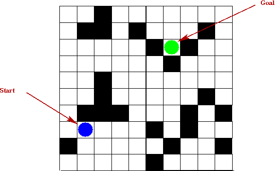
- The maze is an N x N grid of cells.
- Each cell is either closed (prohibited) or not.
- There is a start cell and a goal cell.
- At each step, the allowable actions are: take one step (one cell)
in one of four directions North, South, East, West.
- For example, the following sequence works for the above
instance of the problem:
W, N, N, N, N, N, E, E, E, N, N, E, E, E, S, S
- The algorithmic problem: write an algorithm that produces
a sequence of actions when given the start and end configurations.
- Secondary goal: find an efficient (short) sequence.
- The N-puzzle problem
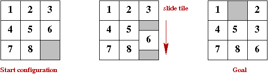
- The example shows an 8-puzzle.
- There are 8 tiles in 9 spaces.
- A "move" (action) consists of moving a tile into the blank
spot (leaving another blank spot).
- The objective: find a sequence of actions to go from the
initial configuration to the goal.
- The algorithmic problem: write an algorithm to do so.
- Secondary goal: find an efficient (short) sequence.
- The robot arm problem:
- Given an N-link arm, a start configuration and an
end configuration, find a sequence of moves to go from
start to end.
- The algorithmic problem: write an algorithm to do so.
- Secondary goal: find an efficient (short) sequence.
Exercise 2:
Download and unpack planning.jar,
then execute PlanningGUI. Familiarize yourself with the
three planning problems, and experiment with different goal
configurations: generate "easy" and "hard" configurations to reach
from the initial configuration. How can you tell what's
easy or hard?
About planning problems in general:
- Many problems have a set of desired goals
⇒
In such problems, one needs to find any one goal.
- In real-time planning problems, some data could
change with time
⇒
e.g., measurements from robot sensors
- Real-world planning problems combine a variety of data
(some noisy) and constraints (time-constraints)
⇒
e.g., motion planning on-the-fly
- Real-world planning problems combine various levels:
⇒
short-term motor control to high-level multi-robot coordination
2.2 State spaces and neighborhoods
Sometimes we use state instead of configuration:
- A state can be a more numeric description than a configuration.
⇒
e.g., use precise coordinates for arm-joint positions.
- The set of allowable actions may depend on the state
⇒
e.g., cannot move "South" when in the bottom row of the maze problem
Exercise 3:
Find a goal state for the arm problem.
How does one specify a complete description of this state?
Exercise 4:
How many possible states are there for each of the three problems?
A neighborhood:
- Each action taken in a given state leads to another state
⇒
That other state is a neighbor of the first state.
- The neighborhood of a state is the set of possible states
reachable from the state using actions allowed in that state.
- A neighborhood may not be spatially contiguous:
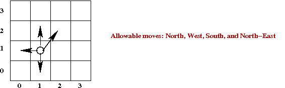
- Here, no sharp right turns are permitted (perhaps because
of the vehicle's limitations).
- Thus, the cell to the east is not a neighbor.
Exercise 5:
What is the size of the neighborhood for each of the three
problems?
Exercise 6:
Consider the starting state in the 8-puzzle demo. Draw this state
on paper, draw all its neighbors and all neighbors of its
neighbors.
The underlying graph:
- What is a graph? See this
definition, for example.
- Each planning problem has an underlying graph:
- Each state is a vertex in the graph.
- When an action takes you from one state to a second one,
place a directed edge from the first to the second.
⇒
We will call these edges action edges.
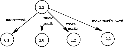
- For example: consider the maze problem with no right-turns:
- From cell (1,1), the neighbors are: (0,1), (1,2), (1,0) and (2,2)
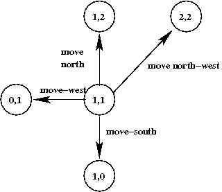
- We need not draw the graph spatially. This is just as accurate:
- The above shows only part of the full graph:
⇒
A full graph would show all possible states and all
possible edges.
- The objective of planning: find a (short) path from
a given start state to a given goal state.
What we know about the shortest-path problem in graphs:
- The shortest-path problem can be solved relatively
efficiently.
- The most efficient algorithm for this problem is
called Dijkstra's algorithm.
See this
description, for example.
- Given a graph with n nodes and m edges, a
careful implementation of Dijkstra's algorithm can find a
shortest path in time O(m log(n)) time.
Unfortunately ...
- Planning problems often have very large numbers of states
⇒
e.g., the N-puzzle problem has O(N!) states.
- It's usually infeasible (and unnecessary) to generate the
whole graph ahead of time.
The approach taken by planning algorithms:
- Generate states on the fly (incrementally).
- Store some states but not all.
Before looking at planning algorithms, let's examine the
output of a planning algorithm.
Exercise 7:
Compile and load MazeHandPlanner into PlanningGUI for the
maze problem.
- Click on "Plan" and then click on "Next" repeatedly
to see what this algorithm produced.
- Examine the code in MazeHandPlanner. Create a different maze
to solve, and hand-code the solution in MazeHandPlanner.
- Examine the code in PuzzleHandPlanner. Observe how
states are generated and entered into the plan.
2.3 Non-cost methods: BFS and DFS
First, we'll explain how BFS and DFS work
⇒
It'll become clear why they are "non-cost"
Note: BFS = Breadth-First-Search, DFS = Depth-First-Search
Key ideas:
- We will consider the (unbuilt) graph of states and action-edges.
- Instead of generating the whole graph, we will create nodes
and edges as we proceed.
⇒
Turns out, we will not need to store edges.
- Use two data structures:
- Visited: a collection of nodes (states) that we
have "finished processing"
- Frontier: a collection of nodes that we have
partially processed.
- At each step:
- Pick a node from Frontier.
- Examine action-edges from that node.
- If there are neighbors that are unexplored, add them to frontier.
- Stop when you find the goal, or when you are out of memory.
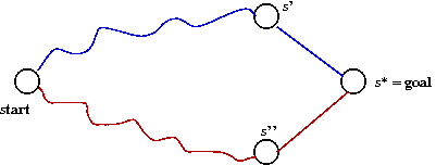
- Here is an example snapshot:
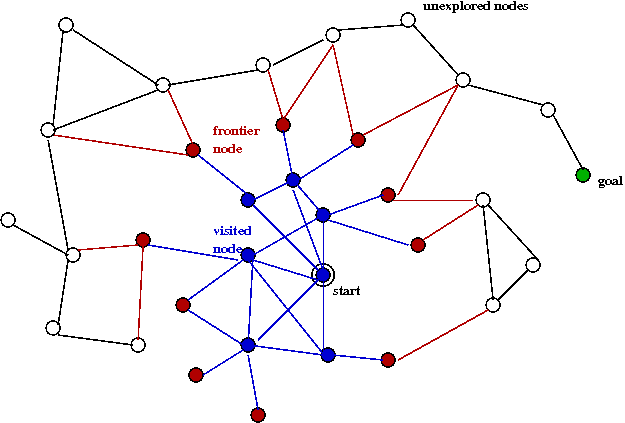
- The blue nodes are in Visited.
- The red nodes are in the Frontier.
- The black nodes are nodes not yet explored (or even generated).
- BFS and DFS differ in their selection of which frontier
node to process next.
- BFS: Frontier is a queue.
- DFS: Frontier is a stack.
- Pseudocode for BFS:
    Algorithm: BFS (start, goal)
    Input: the start and goal nodes (states)
    1.   Initialize frontier and visited
    2.   frontier.add (start)
    3.   while frontier not empty
    4.       currentState = frontier.removeFirst ()
    5.       if currentState = goalState
    6.           path = makeSolution ()
    7.           return path
    8.       endif
    9.       visited.add (currentState)
    10.      for each neighbor s of currentState
    11.          if s not in visited or frontier
    12.              frontier.add (s)
    13.          endif
    14.      endfor
    15.  endwhile
    16.  return null               // No solution
Exercise 8:
Compile and load BFSPlanner into PlanningGUI for the
maze problem. Verify that it finds the solution by clicking
on the "next" button once the plan has been generated.
Likewise, apply BFS to an instance of the puzzle problem
and verify the correctness of the plan generated.
Exercise 9:
Implement DFS by modifying the BFS code.
- Compare BFS and DFS using a variety of puzzle-problem instances.
- Identify both the number of moves (time taken) and the
number of steps in the path.
- Write recursive pseudocode for DFS. Is there an advantage
(or disadvantage) to using recursion?
Exercise 10:
Compare the memory requirements of BFS and DFS. In general,
which one will require more memory? Can you analyze (on paper)
the memory requirements for each?
Exercise 11:
Examine the use of the two data structures in BFS and DFS.
Identify the operations performed on each of these.
How much time is taken for each operation performed
on these data structures? Are there data stuctures
which take less time?
2.4 Cost-based methods
The problem with BFS/DFS:
- Neither of them use any knowledge of the problem.
⇒
e.g., in the maze problem, it's easy to calculate the distance to the goal.
- Both can end up wasting time by searching "away from the goal."
Cost-based methods:
- Recall: one objective of a planning algorithm is to identify
the plan with the least number of "moves" (lowest cost).
- What is "cost"?
- For most planning problems: cost is the number of moves
from the start state.
- Some planning problems include the realization cost (some
actions may take more time).
The Cost-Based-Planner (CBP) Algorithm:
- From among the Frontier nodes, pick the one with the least
total cost from the start state.
- Whenever a state is added to the Frontier, see if the
cost to that state has been reduced.
- Pseudocode:
    Algorithm: CostBased (start, goal)
    Input: the start and goal nodes (states)
    1.   Initialize frontier and visited
    2.   frontier.add (start)
    3.   while frontier not empty
    4.       currentState = remove from frontier the state with least cost
    5.       if currentState = goalState
    6.           path = makeSolution ()
    7.           return path
    8.       endif
    9.       visited.add (currentState)
    10.      for each neighbor s of currentState
    11.          if s not in visited and not in frontier
    12.              frontier.add (s)
    13.          else if s in frontier
    14.              c' = cost to s via currentState
    15.              if c' < current cost of s
    16.                  current cost of s = c'
    17.              endif
    18.          endif
    19.      endfor
    20.  endwhile
    21.  return null               // No solution
Exercise 12:
Implement the CBP by adding code to
the method
removeBest()
in
CBPlanner.java that is included in planning.jar.
Most of the code has been written: you only need to extract
the best node from the frontier using the costFromStart
value in each state (which has already been computed for you).
Exercise 13:
Compare BFS with Cost-Based for the puzzle problem.
Exercise 14:
Examine the operations on data structures in CBP.
Estimate the time needed for these operations. Suggest
alternative data structures.
An improvement:
- Note that Cost-Based-Planner (CBP) does not make any use
of the goal state.
⇒
Surely, one should give preference to the neighbors closer to
the goal state?
- The A* algorithm:
⇒
Pick the state whose combined cost-from-start and cost-to-goal
is the least.
- Note:
- The cost-from-start is exact because we compute it
as we go along.
- The cost-to-goal is not known but must be estimated.
Exercise 15:
What is a reasonable estimate of the cost-to-goal for the
maze and puzzle problems? That is, from given a state
and the goal, what is an estimate of how many moves it would
take to get from the state to the goal?
Show by example how the estimate can fail in each case.
Exercise 16:
In a new file called
CBPlannerAStar.java,
copy over your code from CBPlanner
and implement the A* algorithm. Again, you do not need to perform
the estimation. Simply use the estimatedCostToGoal
value in each state (which has already been computed for you).
Exercise 17:
Compare the time-taken (number of moves) and the quality
of solution produced by each of A* and CBP for the
maze and puzzle problems. Generate at least 5 instances
of each problem and write down both measures (number
of moves, quality) for each algorithm.
Exercise 18:
Examine the code that produces the estimatedCostToGoal
for the maze and puzzle problems. Can you suggest an alternative
for the puzzle problem?
2.5 Completeness, optimality and efficiency
What these terms mean:
- Completeness: if there's a solution (path to goal
state), then the algorithm will find it.
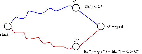
- Optimality: the algorithm finds the least-cost
path to the goal, if at least one path exists.
- Efficiency: the algorithm finds optimal paths
in the least amount of time (its own running time).
Completness:
- All the algorithms we have seen are complete, provided they
don't run out of memory.
- BFS is the most vulnerable
⇒
Memory needs can be exponential in some problems
(Tree example)
- Memory requirements can be reduced by removing
Visited altogether
⇒
Does not affect completeness.
- DFS has the least memory (for Frontier) needs, O(depth)
⇒
O(depth) is rarely large
- CBP and A* eventually search the whole state space
⇒
They are complete.
Optimality:
Efficiency:
- There is no proof that one algorithm is more efficient than another.
- Generally, experimentation shows that A* is more efficient
than CBP, which is more efficient than BFS/DFS.
2.6 Continuous spaces: the arm problem
A challenge with discretizing:
- The arm moves "continuously"
⇒
motors that move joints move in very small steps.
- We could discretize, but at what granularity?
Let's first take a naive approach and fully discretize the space:
- Two options:
- One way to do this is to impose a grid on the space.
- Another way: define discrete "neighbors" for each state.
- We will use the second approach. For each state and each movable joint:
- Define eight neighboring positions
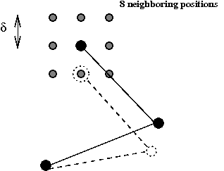
- If the coordinates of a joint are (x, y), then the
new position is potentially (x+dx, y+dy) .
- Here, dx is either 0, δ or -δ.
- Similarly, dy is either 0, δ or -δ.
Exercise 20:
Compare BFS, CBP and A* on the arm problem. Initially, use
a simple target (a short distance up the y-axis). Gradually make
the target harder.
Exercise 21:
Identify the part of the code that computes the neighbors
of a state in ArmProblem.java. Change the 8-neighborhood
to a 4-neighborhood (N,S,E,W) and compare. In the CBP code,
you can un-comment the "draw" line to see what the screen
looks like when the algorithm is in action.
Exercise 22:
How do we know we have visited a state before? How and where
is equality-testing performed in the code? What makes this
equality-test different from the test used in the maze and
puzzle problems?
Next, let's consider discretizing another way:
- We'll break the arm-movement problem into two levels:
- A high level that's discrete.
- A low level that's continuous.
- Key ideas:
- Use a discrete approach to move the arm from one major
configuration to another:
⇒
Example: from "straightened" to "folded"
- Use a continuous "inverse-kinematics" approach for
finer-grained movement.
Inverse kinematics:
Now let's look at a slighly more complex task that combines
high-level discrete states with low-level small changes to angles:
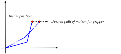
- Suppose a two-link arm is initially folded so that the end
is on the y-axis.
- The final destination: \(x=30, y=10\).
- Suppose, further, that high-level planning (such as A*)
creates the following high-level sequence of actions:
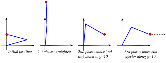
where:
- The arm is first nearly straightened as a precursor to
folding "the other way".
- The second link is brought down to \(y=10\).
- The end is now moved along \(y=10\) until \(x=30\).
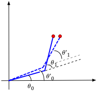
Exercise 24:
Within each of the above phases, identify the signs (positive or negative)
of \(\Delta\theta_0, \Delta\theta_1\). For example, when
straightening, what are the signs of each likely to be?
- We'll then set up our control loop to follow the phases:
    // Initially, state=0
    while not over
        if state = 0
            if (straightened)
                state = 1       // Go to state 1
            else
                apply Δθ0,Δθ1 to straighten
            endif
        else if state = 1
            if y = 10
                state = 2       // Go to state 1
            else
                apply Δθ0,Δθ1 to bring 2nd link down
            endif
        else if state = 2
            if x = 30
                stop
            else
                apply Δθ0,Δθ1 to move horizontally
            endif
        endif
    endwhile
Exercise 25:
Download and unpack
twolinkexample.zip.
- Examine the code in
TwoLinkController.java to
confirm that the above controls are implemented.
- Add code for the last part, to compute \(\theta_1^\prime\),
or newTheta1 in the code
so that the end effector reaches \((30,10)\).
- To execute, run
ArmSimulator,
type in the controller name
"TwoLinkController",
set the number of links (to 2),
then click on "tracing", then "reset", then "go".
In practice:
- It is not at all straightforward to combine high-level
planning and inverse-kinematics.
- Inverse-kinematics calculations are highly dependent on
the particular arm or robot.
- Most inverse-kinematics calculations must also take into
account other complexities, for example:
- Forces and torques for smoother movement, for handling loads.
- Safety: to prevent the arm from crashing into itself.
- Corrections from drift, when model and reality are out of sync.
- Both planning and inverse-kinematics continue to be active
areas of research.
2.7 Other algorithms
Greedy:
- Instead of combining the cost-from-start and
estimated-cost-to-goal, we could use just estimated-cost-to-goal
⇒
Called the Greedy planning algorithm.
- Greedy is neither guaranteed to be complete nor optimal.
- Greedy can be made complete if we make sure that at least
one node from the Frontier is expanded each step.
Exercise 26:
Create an example of the maze problem in which Greedy
performs badly.
Reducing memory requirements:
- There are two commonly-used approaches for reducing
memory-requirements:
- Fix the memory size, and throw out nodes heuristically.
- Re-run an algorithm several times
⇒
Each time, use what was learned in earlier iterations to prune the search space.
- Limiting memory size: SMA* (Simplified Memory-Bounded A*)
- Use A* until memory is full.
- Drop the node with the highest-cost.
- Record this node's cost in its parent.
⇒
So that we don't expand the parent until it becomes necessary.
- Iterative deepening: IDA*
- Fix a cost bound B.
- Apply A* until costs exceed B.
⇒
Let B' = the cost that first exceeded B.
- Set B = B' and re-run.
- Repeat until goal node found.
Other ideas in search:
- There is a whole world of search algorithms, and many
specialized books on the subject.
- Example sub-topics: search for games, realtime-search,
meta-heuristics.
About planning:
- We have only lightly touched upon the general planning problem.
- Planning is a vast area with all kinds of research, books
and products.
- There is an entire sub-area related to planning motion.
- An example of successful planning: Mars Rover mission.
© 2008, Rahul Simha