Satisfiability
Overview
The intersection of computation and logic is both intellecually
interesting and of tremendous practical significance.
Some of the most valuable theoretical developments in
computing have come from this intersection:
- The Church-Turing thesis.
- The theory of NP-completeness.
- Automated theorem proving.
A preview:
- Background and problem definition.
- Some theoretical highlights.
- The DP and DPLL algorithms.
- Hard instances of SAT.
- Local search algorithms.
- The landscape of SAT.
- Elements of modern SAT solvers.
Our presentation will pull together material from various sources - see the
references below. But most of it will come from
[Marq1999],
[Gome2008]
and [Zhan2003].
Background and problem definition
Consider math equations:
- Example:
4x1 - 2x1 + 3x2 - 12 = 0
Does this have a solution?
=> Yes: x1 = 1.5 and
x2 = 2
Note: this equation has multiple solutions, e.g.
x1 = 1 and
x2 = 3.333
- What constitutes an equation?
- An equation has variables like
x1, x2, ...
- There are operators that "act" on the variables.
- Unary operators like x12.
- Binary operators like addition, multiplication.
- General form of an equation:
expression-with-variables = constant
such as
4x1 - 2x1 + 3x2 - 12 = 0
- Some things we know about math equations:
- We can solve linear and quadratic equations easily.
- We can solve some equations invovling high powers.
- We can solve many non-linear equations numerically.
- Some equations (quintics and higher) cannot be solved.
- Some equations have no solution, e.g.
x13 + x23
- x33 = 0
(where xi is an integer)
[Wiles' Not-Last Theorem]
- So far, all of these equations have involved numbers.
Boolean equations:
- These also have the general form
expression-with-variables = constant
- However,
- Variables are Boolean: can take only one of two values (TRUE or FALSE)
xi = T
or
xi = F
- Operators are Boolean operators.
- Only one unary operator (complement):
x'i = opposite value of
xi
We can express this as the truth table:
- Consider these two binary operators: AND and OR
- x1 AND x2 is TRUE
only when both x1
and x2 are TRUE.
- x1 OR x2 is TRUE
when either x1
or x2, or both, are TRUE.
- It's convenient to represent binary operators using
truth tables:
- The table for AND:
| x1 |
x2 |
x1 AND x2 |
| T | T | T |
| T | F | F |
| F | T | F |
| F | F | F |
- The table for OR:
| x1 |
x2 |
x1 OR x2 |
| T | T | T |
| T | F | T |
| F | T | T |
| F | F | F |
Exercise:
How many possible binary operators are there?
- Equation example with AND/OR:
(x'1 AND x2) OR
(x'1 AND x3) = T
Can we find a solution?
Answer: Yes: x1 = F,
x2 = T, x3 = T
Note: this equation has more than one solution:
x1 = F,
x2 = T, x3 = F
- Another example:
(x'1 OR x2) AND
(x1 OR x'2) AND
(x1 OR x2) = T
Turns out: this has no solution
- For brevity, we use + for OR and multiplication for AND:
(x'1 + x2)
(x1 + x'2)
(x1 + x2) = T
- CNF expressions:
- A Conjunctive-Normal-Form (CNF) expression looks like this:
(x'1 + x2)
(x'1 + x3)
- It is a collection of clauses that are AND'ed together.
- Inside each clause, the only binary operator allowed is OR.
- The unary operator can only be applied to variables.
- CNF Equation:
CNF expression = T
- Notation: a literal is an occurence of a variable
in either natural or complementary form, e.g. in
(x'1 + x2)
(x'1 + x3)
- The first literal in this expression is: x'1.
- The second literal in this expression is: x2.
The Satisfiability problem:
- The general Satisfiability problem:
Given an CNF equation, is there a solution?
- The k-SAT variant:
- Each clause is limited to at most k literals.
- Example of a 3-SAT problem:
(x'1 + x2 + x'4)
(x2 + x'3 + x4)
(x1 + x'2 + x3)
(x1 + x2 + x3) = T
- Example of a 4-SAT problem:
(x'1 + x2 + x'4 + x'5)
(x1 + x3 + x'5 + x'6)
(x1 + x2 + x3 + x5)
= T
- The k-SAT problem:
Given an k-CNF equation, is there a solution?
- Equivalently, given a k-SAT expression, is the expression
satisfiable?
What about Boolean equations using operators other than AND/OR?
- Fact: Any Boolean expression with standard
propositional operators can be converted to an equivalent
CNF expression.
→
CNF expressions are not restrictive.
- What does equivalent mean?
- Suppose E is a Boolean expression.
- Let CNF(E) be the equivalent expression in CNF.
- Then E is true if and only iff CNF(E) is true.
- So, what are these "standard" operators?
→
NAND, IMPLIES ... all 16 possible binary operators (and complement).
Consider DNF: Disjunctive Normal Form
- An expression is in DNF if:
- It consists of clauses that are OR'd together, e.g.,
(x'1 x2 x'4) +
(x2 x'3 x4) +
(x1 x'2 x3) +
(x1 x2 x3)
- Each clause has only AND'ed literals.
Exercise:
Give a polynomial-time algorithm to test whether a DNF expression
is satisfiable.
- Fact: any Boolean expression can be converted into a DNF equivalent.
- So, couldn't we convert CNF into DNF and determine satisfiability?
- CNF to DNF conversion essentially "multiplies out" the
clauses, e.g.,
(x'1 + x2)
(x1 + x3)
=
x'1 x1 +
x'1 x3 +
x2 x1 +
x2 x3
Exercise:
Consider the CNF expression
(xa1 + xb1)
(xa2 + xb2)
...
(xan + xbn)
- How many variables does this expression have?
- What is the size of the equivalent DNF expression?
- Thus, even though DNF can solved quickly, the time
taken for CNF to DNF conversion can be exponential.
Other types of operators:
- Consider the quantifier operators ∀ and ∃ as in
∀ x1 ∃ x2
(x'1 + x2)
(x1 + x3)
- Expressions with the usual propositional operators
and also the quantifiers are called Quantifiable Boolean
Formulas.
- QBF satisfiability is a harder problem (P-SPACE complete).
- When you add predicates to QBF's you get
expressions in first-order logic
- In general, the satisfiability question for first-order logic
is undecidable.
Applications:
- SAT is not merely of theoretical importance
→
There are many useful applications.
[Marq2008].
- Circuit testing: is a designed circuit equivalent
in function to the original design?
- Model-checking:
- Given a finite-state model and transition rules,
does the system reach an undesirable state?
- Model-checking can be applied to algorithms, to
hardware, to systems in general.
- Planning:
- A problem that originated in AI.
- Certain planning problems can be expressed as SAT problems.
- Automated theorem proving.
Some theory
The Cook-Levin theorem:
- Originally ascribed to Stephen Cook along, based on his
landmark 1971 paper.
- Was a "curiosity" until Richard Karp showed many (21 or so)
important optimization problems were reducible.
- Later, it was discovered that the Russian Leonard Levin
had developed similar ideas but in the framework of search problems.
- We will outline the broad ideas in the proof.
- First, we'll need to understand what the decision
version of a combinatorial problem is:
- Consider TSP, which is usually stated as: given a
collection of points, find the minimum-length tour.
- The decision version: Given a collection of
points and a number L, is there a tour of length
less than L?
- About decision versions:
- The output is either "yes" or "no".
- Typical optimization version: "Given input ... minimize the
cost function".
- Corresponding decision version "Given input ... and a number
C, is there a solution with cost no more than C?".
- Is the decision version easier?
- It certainly appears so. But ...
- Suppose we have a decision-version algorithm for TSP that
takes time P(n).
- Given input, it answers the question "is there a tour of
length at most L?".
- To find a minimal length tour, start with these questions
- Is there a tour of length 0?
- Find any tour, of length L', say. Question: is
there a tour of length L'?
- Then, use binary search between 0 and L'.
=> can "hone in" on optimal solution in time O(P(n) log (L)).
=> most likely polynomial in n.
- Define the class of NP problems as:
A (decision) problem is in NP if there is a non-deterministic Turing
machine that can solve it in polynomial time.
- What does non-deterministic mean here?
- Recall what a deterministic Turing machine is:
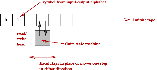
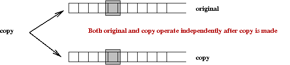
- In a non-deterministic Turing machine, a copy of the
machine can be made to "try a variation of the current solution".
- Intuitively, if we are solving TSP:
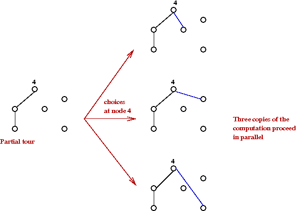
- Given a TSP instance, we want one of these to answer
the decision question (tour ≤ L) in polynomial time.
- So, is TSP in the class NP?
→
Most assuredly
- Simply try all possible tours non-deterministically.
- Each individual copy runs in polynomial-time.
- We already know the polynomial (and therefore, the time bound).
→
We can halt the copies that exceed the bound
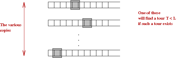
- If there is a tour with cost ≤ L, one of these
will halt with "yes".
- Let's use the term clone for each individual
copy during a "run" of a non-deterministic Turing machine.
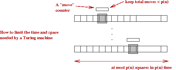
- Let p(n) be the polynomial bound for TSP
→
The max # steps needed by a non-deterministic Turing machine
to "decide".
- Important: n is the size of the problem (number of TSP points).
- Now, in time p(n), a Turing machine can only process
at most p(n) squares.
- If we were to make a movie of the Turing machine,
we can list the possible frames in a grid of size
at most p(n)2.
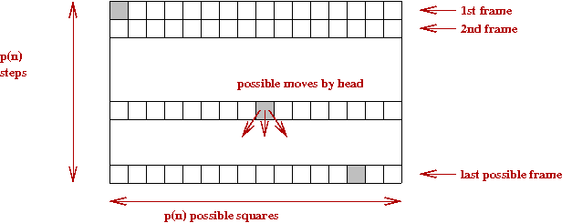
- The connection with satisfiability:
- We will create a huge but polynomial number (of the
order of p(n)2) Boolean variables.
- The Boolean variables will be connected using Boolean
operators into a CNF expression C.
- C will be true if and only if there is a clone
that says "yes".
- The construction is elaborate:
- Need variables to capture possible tapehead moves.
- Need variables to capture completion (final state).
- Need variables for all possible squares at all possible times.
- Totally, O(p(n)3) variables.
- Thus, if a SAT-solver can guarantee solution in polynomial-time,
it can solve the decision version of TSP in polynomial-time.
- In fact, if a polynomial SAT-solver exists, it can solve
the decision problem for any NP problem
→
This is the Cook-Levin theorem.
2-SAT:
- Cook's theorem used large CNF formulas.
- This raises the question: can k-SAT be solved for any fixed
k?
- Turns out, for any CNF expression C, you can
construct a corresponding 3-CNF expression C' such
that:
C is satisfiable if and only if C' is satisfiable.
- But 2-SAT? 2-SAT is polynomially solvable.
→
An algorithm due to Apvall, Plass and Tarjan
[Apsv1979].
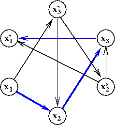
- Let's see how this works with an example. Consider
the 2-CNF formula
(x'1 + x2)
(x'2 + x3)
(x3 + x2)
(x'3 + x'1)
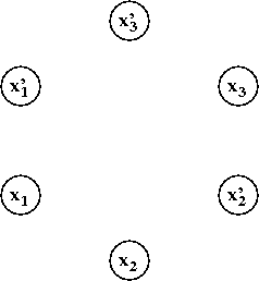
- We build a graph with vertices
xi and x'i
for each i:
- For every clause, add two edges:
- Consider the clause (x'1 + x2).
- Add the edge "complement of first to second":
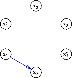
- Add the edge "complement of second to first"
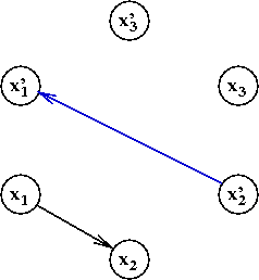
Exercise:
What edges do we get for the second clause?
- Thus, for the above example, the resulting 8-edge graph is:
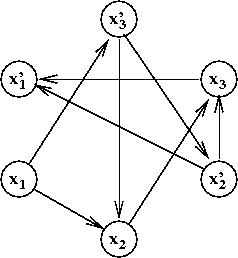
- Now ask the question: is there a variable xi
such that there is both
- a path from xi to
x'i
- and a path from x'i to
xi?
If so, the CNF formula is NOT satisfiable.
- In the above example, there is a path from
x1 to x'1:
Let's examine what this means when x1=T
- The arc (x1, x2) says
"If x1=T then I must set
x2=T"
- Why? The arc is there because of a clause
(x'1 + x2).
- Similarly, the arc (x2, x3) says
"If x2=T then I must set
x3=T"
- Similarly, the arc (x3, x'1) says
"If x3=T then I must set
x'1=T"
→
A contradiction!
- Similarly, if there were a path from
x'1 to x1
it would mean "You can't set x'1=T."
→
Which would mean the clause is unsatisfiable.
- Can paths be checked efficiently?
→
Yes, depth-first search from each variable.
Exercise:
Add some clauses to make the above 2-CNF formula unsatisfiable.
- What about the other direction?
→
If there are no such dual-paths, how does one construct
a satisfiable assignment?
- Find an unassigned variable and assign it to true (and its
complementary vertex to false).
- Follow its paths, assigning true by implication.
- Repeat.
The DP and DPLL algorithms
The Davis-Putnam algorithm
[Davi1960].
The Davis-Putnam-Logemann-Loveland (DPLL) algorithm:
[Davi1962].
- Historical note:
- Although the paper is co-authored by Davis, Logemann and Loveland,
the algorithm is often called DPLL (including Putnam).
- Davis and Putnam are better known for their solution
to Hilbert's 10th problem: the unsolvability of
diophantine equations
- First, consider a simple exhaustive search:
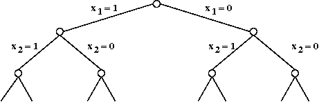
- Consider the example
(x'1 + x3)
(x2 + x'4 + x'5)
(x'3 + x'4)
(x2 + x4 + x5)
- With 5 variables, there are 25
possible solutions to try
→
Of course, one could find a satisfying solution sooner.
- Now, consider the following with the same example:
(x'1 + x3)
(x2 + x'4 + x'5)
(x'3 + x'4)
(x2 + x4 + x5)
- Suppose we try x1=T in the formula above. This gives
(F + x3)
(x2 + x'4 + x'5)
(x'3 + x'4)
(x2 + x4 + x5)
- Which simplifies to:
(x3)
(x2 + x'4 + x'5)
(x'3 + x'4)
(x2 + x4 + x5)
- We now have a unit-clause which forces
an assignment to the variable inside
→
We must set x3=T.
- This in turn results in:
(T)
(x2 + x'4 + x'5)
(F + x'4)
(x2 + x4 + x5)
- Which forces x4=F:
(x2 + T + x'5)
(T)
(x2 + F + x5)
- ... and so on. (This formula was satisfiable).
- Consider this example:
(x'1 + x'3)
(x2 + x'5)
(x3 + x4)
(x3 + x'4)
- Suppose we set x1=T to get
(x'3)
(x2 + x'5)
(x3 + x4)
(x3 + x'4)
- Now, we are forced to set x3=F to get:
(x2 + x'5)
(x4)
(x'4)
- Which forces x4=T to get:
(x2 + x'5)
(T)
(F)
→
A contradiction.
- Which means the formula is unsatisfiable.
- When a literal becomes false, we remove it from
a clause.
- For example, in the example above, we set x1=T in
(x'1 + x'3)
(x2 + x'5)
(x3 + x4)
(x3 + x'4)
to get
(F + x'3)
(x2 + x'5)
(x3 + x4)
(x3 + x'4)
- This effectively removes x1 from the first clause:
(x'3)
(x2 + x'5)
(x3 + x4)
(x3 + x'4)
- Similarly, when we set x3=F in
(x2 + x'5)
(x4)
(x'4)
we get the empty clause
(x2 + x'5)
(T)
()
- Thus, the general idea is:
- Choose an unassigned variable and assign it a value (T or F).
- See if this creates unit-clauses, which forces variable
assignments.
- Whenever a variable is set to a value:
- It could make some clauses become "true"
→
In this case, remove the whole clause.
- It could result in a "F" value inside a clause
→
In this case, remove the variable from those clauses.
- If at any time, we get an empty clause, the formula is unsatisfiable.
- Pseudocode:
      Algorithm DPLL (F)
      Input: A formula (set of clauses) F defined using variables in a set V

      1.   if F is empty
      2.     return current assignment     // Found a satisfying assignment.
      3.   endif

      4.   if F contains an empty clause
      5.     return null                   // Unsatisfiable.
      6.   endif

           // One variable => no choice, really, for that variable.
      7.   if F contains a clause c with only one variable v
      8.     Set the value of v to make c true
             // One TRUE variable is enough to make c TRUE
      9.     F' = F - c
             // Call DP recursively on the remaining clauses.
     10.     return DPLL(F')
     11.   endif

           // Try both TRUE and FALSE for an unassigned variable.
     12.   v = variable in V which has not been assigned a value

           // Try TRUE first
     13.   v = TRUE
     14.   F' = simplify F accounting for v's new value
     15.   if DPLL(F') is satisfiable
     16.     return current assignment
     17.   endif

           // OK, that didn't work. So try FALSE next.
     18.   v = FALSE
     19.   F' = simplify F accounting for v's new value
     20.   if DPLL(F') is satisfiable
     21.     return current assignment
     22.   else
             // If it can't be done with either, it's unsatisfiable.
     23.     return null
     24.   endif
- The very essence of DPLL can be boiled down to two phases:
unit-clause propagation and exploration
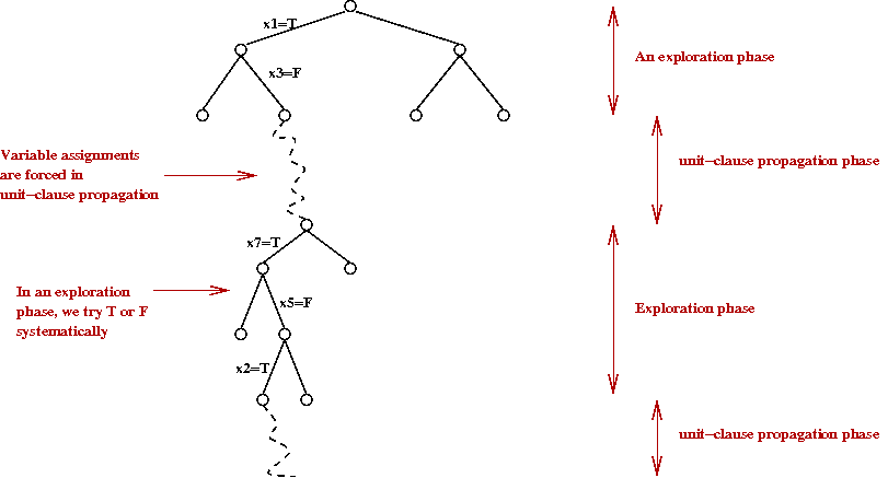
- Thus, in some sense, the pseudocode can be simplified to:
     1.   check for end-of-recursion
     2.   propagate unit-clauses
     3.   explore
Exercise:
How how DPLL can be written iterative (non-recursive) form.
Hard instances of SAT
Consider this approach to generating a random graph:
- Draw n vertices:
- Then, for each possible pair of vertices in turn:
- Flip a coin.
- If "heads", place an edge between the two vertices.
- In our example:
- 21 possible pairs:
(1,2), (1,3), (1,4), (1,5), (1,6), (1,7)
(2,3), (2,4), (2,5), (2,6), (2,7)
(3,4), (3,5), (3,6), (3,7)
(4,5), (4,6), (4,7)
(5,6), (5,7)
(6,7)
- Suppose we happen to get 9 heads on our 21 coin tosses:
(1,2), (1,3), (1,4), (1,5), (1,6), (1,7)
(2,3), (2,4), (2,5), (2,6), (2,7)
(3,4), (3,5), (3,6), (3,7)
(4,5), (4,6), (4,7)
(5,6), (5,7)
(6,7)
- The result is a graph.
Observe: the graph is connected
=> There's a path between every two vertices.
- Note:
- If we repeated the experiment, we would probably get
a different set of coin results, and therefore a different graph.
- Here, we assumed Pr[heads] = 0.5.
- Biased coins:
- Suppose Pr[heads] = p instead, where p=0.1 or
p=0.95 is possible.
- How likely is it that we will get a connected graph
if p = 0.1?
- How likely is it that we will get a connected graph
if p = 0.9?
- Let q = Pr[Graph is connected].
Question: how does q depend on p.?
- One might think:
- But actually,
- Celebrated result (Erdos and Renyi):
- If p < 1/n, the graph is almost always disconnected.
- If p > log(n)/n, the graph is almost always connected.
- If 1/n < p < log(n)/n, the graph has a giant connected component.
=> Example of a phase transition phenomenon.
- Other examples of phase transitions:
- Water to ice.
- Site/bond percolation.
- Superconductivity.
Now let's come back to the k-SAT problem:
- Recall problem: given a k-SAT CNF equation, does a solution exist? e.g.,
(x'1 OR x2 OR x'4) AND
(x2 OR x'3 OR x4) AND
(x1 OR x'2 OR x3) AND
(x1 OR x2 OR x3) = T
- Recall DPLL heuristic:
- Successively break problem into smaller parts (fewer clauses)
and try T/F assignments to variables.
- Eliminate clauses where possible.
Random k-SAT instances:
- We will create random k-SAT equations for DP to solve.
- Let L = ratio of #clauses to #variables.
- Let C = number of recursive calls made by DP.
- Goal: plot average value of C vs. L.
- Surprising result: A phase transition
[Mitc2005].
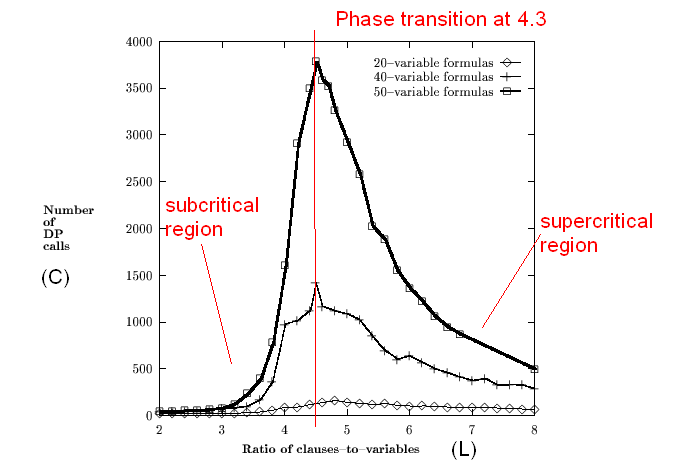
(Reproduced from: D.G.Mitchell, B.Selman, H.J.Levesque. Hard
and easy distributions for SAT problems. Proc. Nat.Conf.AI, 1992).
- Such a phase transition has also been observed
in other random-SAT models
[Gent1993].
State-based local search
State-based local search is an idea that works
well for many combinatorial optimization problems:
- The idea is to start with potential solution
and repeatedly improve the solution.
- For the Traveling Salesman Problem (TSP):
- Start with a random tour.
- Perform a cost-improving 2-edge swap.
- Repeat.
- A similar idea can be used for SAT:
[Selm1992],
[Selm1995].
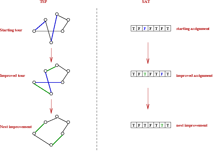
- Start with an assignment.
- Try to "improve" the assignment.
- Repeat until you find a valid assignment.
- What does "improve" mean in this case?
→
Either an assignment satisfies or it doesn't.
- A simple heuristic: pick a variable (and its value)
that decreases the number of unsatisfied clauses.
An example:
- Consider the formula
(x'1 + x2 + x3)
(x'1 + x5)
(x1 + x'3 + x'4)
(x'2 + x5)
(x'2 + x3 + x'4)
(x'1 + x'4)
- Suppose we start with the random assignment
| |
x1 |
x2 |
x3 |
x4 |
x5 |
# unsatisfied
clauses |
| Step 1: |
T | T | F | T | F |
4 |
With this assignment, there are 4 unsatisfied clauses.
(x'1 + x2 + x3)
(x'1 + x5)
(x1 + x'3 + x'4)
(x'2 + x5)
(x'2 + x3 + x'4)
(x'1 + x'4)
- At this step, let's see what each possible "flip" buys us
(in terms reducing unsatisfied clauses):
	 x1 → F  results in 2 fewer unsatisfied clauses.
	 x2 → F  results in 1 fewer unsatisfied clauses.
	 x3 → T  results in 1 fewer unsatisfied clauses.
	 x4 → F  results in 2 fewer unsatisfied clauses.
	 x5 → T  results in 2 fewer unsatisfied clauses.
- Let's say we pick x1 → F
| |
x1 |
x2 |
x3 |
x4 |
x5 |
# unsatisfied
clauses |
| Step 1: |
T | T | F | T | F |
4 |
| Step 2: |
F | T | F | T | F |
2 |
- Once again, we try each possible variable flip:
	 x1 → T  results in -2 fewer unsatisfied clauses.
	 x2 → F  results in 2 fewer unsatisfied clauses.
	 x3 → T  results in 0 fewer unsatisfied clauses.
	 x4 → F  results in 1 fewer unsatisfied clauses.
	 x5 → T  results in 1 fewer unsatisfied clauses.
- The obvious choice is x2 → F
| |
x1 |
x2 |
x3 |
x4 |
x5 |
# unsatisfied
clauses |
| Step 1: |
T | T | F | T | F |
4 |
| Step 2: |
F | T | F | T | F |
2 |
| Step 3: |
F | F | F | T | F |
0 |
→
This satisfies the formula.
Exercise:
In the above approach, when do we know that a formula is NOT satisfiable?
More details:
- It may turn out that we are "wandering in state space"
nowhere near the solution.
- Just as in combinatorial optimization problems, we
might get "stuck" in a local minima:
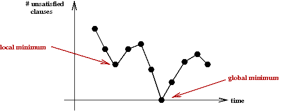
- An idea: re-start with a new random assignment.
- Let's put this into pseudocode:
     Algorithm: Greedy-SAT (F)
     Input: a CNF formula F
     1.   for i=1 to maxTries
     2.      A = a randomly generated assignment
     3.      for j=1 to maxFlips
     4.         if A satisfies F
     5.            return A       // Done.
     6.         endif
     7.         A = Greedy-Flip (A, F)
     8.      endfor
     9.   endfor
          // Give up.
     10.  return "No satisfying assignment found"
     Algorithm: Greedy-Flip (A, F)
     Input: an assignment A and a CNF formula F
          // See how much each variable-flip independently reduces # unsatisfied clauses.
     1.   for k=1 to n
     2.       βk = reduction in unsatisfied clauses by flipping variable xk
     3.   endfor
     4.   Let xm be the variable with the maximum β value.
     5.   if βm > 0
             // Create a new assignment with variable m flipped.
     6.      A = flip (A, m)
     7.   endif
     8.   return A
- Here, the flip(A,k) operation denotes the flipping
the value of variable xk in the assignment A.
- What about correctness?
- Even if there's a satisfying assignment, it may not be found.
- If the formula is unsatisfiable, we'll never know. (We don't keep track of all assignments).
- Thus, the algorithm is not complete.
Exercise:
Notice the condition β>0 in line 5 of Greedy-Flip. What would be
the implication of making this β≥0?
Some improvements:
- Experimental results show that Greedy-SAT gets stuck
in local minima.
- To get out of local minima, replace the condition
in line 5 with β≥0.
- This allows moving to assignments "of the same value."
→
Called a sideways move.
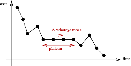
- The idea is to explore more of the state space.
- To allow even more exploration, make occasional "random"
moves.
- At each move, with probability p, simply flip the value
of some variable in an unsatisfied clause (which will satisfy it).
- With probability (1-p), apply the Greedy-SAT move.
- In pseudocode:
     Algorithm: Random-Walk-SAT (F)
     Input: a CNF formula F
     1.   for i=1 to maxTries
     2.      A = a randomly generated assignment
     3.      for j=1 to maxFlips
     4.         if A satisfies F
     5.            return A
     6.         endif
     7.         if uniform() < p       // With probability p
     8.            xk = a randomly selected variable in a randomly selected unsatisfied clause
     9.            flip (A, k)
     10.        else                   // With probability 1-p
     11.           Greedy-Flip (A, F)
     12.        endif
     13.     endfor
     14.  endfor
- An extreme version of this algorithm: when p=1
- Note: in the "random move" part, the algorithm may in fact
increase the number of unsatisfied clauses
→
An increase in "cost".
- This is similar to simulated annealing.
- Simulated annealing can also be made to work for SAT.
- Note: in the Random-Walk-SAT, the greedy move is applied
to any variable.
- We can instead focus on only the variables in unsatisfied clauses.
→
Called Walk-SAT.
- Define for any variable x
b(x) = breakcount(x) = the number of satisfied clauses that become unsatisfied when x is flipped.
- The Walk-SAT algorithm:
     Algorithm: Walk-SAT (F)
     Input: a CNF formula F
     1.   for i=1 to maxTries
     2.      A = a randomly generated assignment
     3.      for j=1 to maxFlips
     4.         if A satisfies F
     5.            return A
     6.         endif
     7.         C = a randomly selected unsatisfied clause.
     8.         xk = the variable in C with the smallest b(xk)
     9.         if b(xk) = 0
     10.            flip (A, k)                   // Greedy move.
     11.        else if uniform() < 1-p
     12.           flip (A, k)                    // Alternative greedy move.
     13.        else                              // With probability p
     14.         xm = a randomly selected variable in C
     15.         flip (A, m)                      // Random walk move.
     16.        endif
     17.     endfor
     18.  endfor
Experimental results:
(reported in
[Selm1995])
- On "hard" instances (at the phase transition):
- DPLL cannot solve when n ≥ 400.
- Walk-SAT performs best (even better than simulated annealing).
- Example from data with 600 variables and 2550 clauses:
- Greedy-SAT took 1471 seconds and needed 30 x 106 flips.
- Walk-SAT took 35 seconds and needed 241,651 flips.
- Simulated annealing took 427 seconds and needed 2.7 x
106 flips.
- However, the distinction is less clear on some data sets
produced from some practical problems.
→
Which might mean the practical problems are "easy".
Other algorithms:
Landscapes and backbones
The above raises interesting questions about SAT instances:
- Do local minima occur often?
- What is the structure of the landscape of hard SAT problems?
- Can one tune algorithms to particular problem instances?
A study about the importance of "greed" and "randomness"
[Gent1993]:
- One can control the amount of "greed"
- For high greed: prefer sharp downhill moves with high probability.
- For low greed: allow uphill or sideways moves frequently.
- Turns out: greed is not as important as allowing sideways moves.
- How much does randomness help?
- Again, one can tradeoff randomness against "fairness".
- Fairness: make sure every variable gets a turn to "flip".
- You can have "high randomness, low fairness", and
also "high fairness, low randomness"
- Turns out: fairness is more important.
Tuning algorithm parameters
[McAl1997]:
- All the state-space search algorithms tradeoff
exploration (randomness) vs. exploitation (greed).
- Algorithms use a parameter, e.g., p in
Random-Walk-SAT, to control the tradeoff.
- The problem: performance on a particular instance is
highly dependent on p.
- On the other hand: we don't know ahead of time what
value of p is best for a particular instance.
- An interesting idea: tune p by learning
a "little" about a particular instance:
- Given an instance, run the algorithm for a while.
- Learn something about the instance.
- Adjust p for remainder.
- First, some observations from experiments:
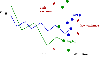
- Let C = final cost when algorithm stops = #
unsatisfied clauses.
- When p is low: Var[C] is low (good
consistency), but E[C] is high.
is low.
- Similarly, you occasionally get lower C, but Var[C]
is high (poor consistency).
- Now, let p* be the optimal value of p.
- Experimentally, it turns out: low p < p*
< high p.
- The problem: how do we know this in advance?
- A key experiment:
- For each instance, estimate optimal p*.
→
Note: p* differs for each instance.
- Also estimate mean-to-variance ratio
E[C*] / Var[C*] at this
value of p*.
- Interesting discovery: E[C*] / Var[C*]
appears to be independent of algorithm and instance.
- Call this number γ = E[C*]/Var[C*].
- γ is like a universal constant.
- The implication:
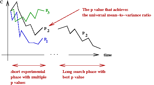
- Over a short run for a single instance,
try different values of p
- Pick the p that produces E[C]/Var[C] = γ.
- Use this value of p for the remainder of that instance.
The backbone of an instance:
[Mona1999]:
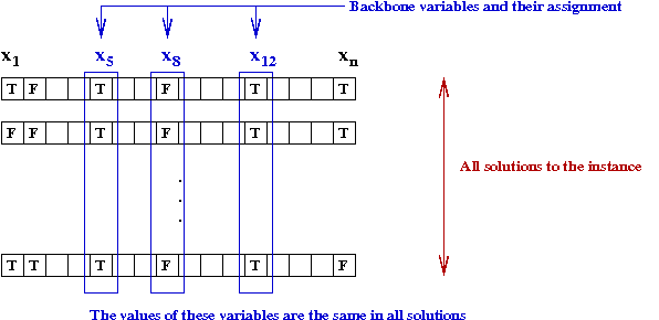
- Experimental evidence shows that for hard instances,
a subset of variables has the same values across all solutions
→
called the backbone of the instance.
- If you knew the backbone variables
you'd need to find their unique assignment first.
- Use DPLL on these variables first.
- The rest of DPLL will probably find a solution quickly.
- How to estimate the backbone?
[Dubo2001]:
- Examine groups of clauses and variables in them.
- Estimate "variability" of a variable by seeing whether
it could possibly appear in multiple solutions.
- Low "variability" might indicate backbone.
- Search backbone variables first (by applying DPLL).
- A related idea: backdoor variables:
- These are a subset of variables such that if you had their
optimal values
→
searching for the remaining variable values takes poly-time.
- Generally, this is smaller than the backbone or might
not involve the backbone at all.
- Unfortunately, there appears to be no general method
for identifying backdoor variables.
Beyond DPLL: modern SAT-solvers
Although modern SAT solvers vastly outperform DPLL (million variables
vs. a few hundred), they are all based on DPLL itself.
First, let's re-write DPLL iteratively:
- Recall the basic structure of DPLL:
         DPLL (F)
         1.   See if recursion has bottomed out (determine satisfiability)
         2.   Pursue unit-propagation to see if a contradiction occurs
         3.   if not
         4.       find an unassigned variable x
         5.       recurse with x=TRUE
         6.       if that didn't work, recurse with x=FALSE
         7.   endif
- Thus, some variable values are chosen (assigned) and others get forced (from clauses that become unit clauses).
- To help understand the improvements to DPLL, we will write
DPLL iteratively (which is the commonly used approach).
      Algorithm: DPLL-Iterative (F)
      Input: A formula (set of clauses) F defined using variables in a set V
     1.    formulaStack.push (F)
     2.    while formulaStack not empty
     3.        status = deduce ()          // Pursue unit-clauses, and see if there's a conflict.
     4.        if status = SATISFIABLE
     5.            return assignment
     6.        else if status = CONFLICT
     7.            backtrack ()
     8.        else
     9.            decideNextBranch ()     // status=CONTINUE so continue trying variable values.
     10.       endif
     11.   endwhile
     12.   return null                     // Unsatisfiable.

     deduce ()
     1.   F = formulaStack.peek ()
     2.   while there is a unit-clause
              // Pursue the chain of unit clauses.
     3.      set the clause's variable to make the clause TRUE
     4.      if contradiction found
     5.         return CONFLICT
     6.      endif
     7.   endwhile
     8.   if no more clauses
     9.      return SATISFIABLE
     10.  else
     11.     F' = simplified formula after unit clauses
     12.     replace F with F' on top of formulaStack
     13.     return CONTINUE
     14.  endif

     backtrack ()
     1.   while true
     2.       F = formulaStack.pop ()
     3.       v = variableStack.pop ()
     4.       if v = TRUE
                  // We've tried v=TRUE, and next need to try v=FALSE.
     5.           v = FALSE
     6.           F' = F simplified with v = FALSE
     7.           formulaStack.push (F')
     8.           variableStack.push (v)
     9.           return
     10.      endif
     11.  endwhile

     decideNextBranch ()
     1.   F = formulaStack.pop ()
     2.   v = a randomly selected unassigned variable
     3.   v = TRUE
     4.   F' = F simplifed with v=TRUE
     5.   formulaStack.push (F')
     6.   variableStack.push (v)
- Note:
- We are using two stacks, one for simplified formulas and one
for variable assignments
→
These mimic the natural stack used in the recursive version.
- Recall: the recursive version used the same recursion to
simplify unit-clauses
→
Here, in deduce(), we follow-through unit clauses in a separate loop
- The iterative version is somewhat harder to understand (and write).
Main ideas in improving DPLL:
- Idea #1: Add new clauses to formula during execution:
- At first this sounds like a radical idea
→
Wouldn't adding more clauses complicate or change the problem?
- The clauses we add cannot change the solution of the
original formula.
- We will add clauses to "force" some conflicts to be
dealt with sooner
→
Instead of spinning wheels until the conflict occurs.
- This is sometimes called conflict-directed clause learning.
- How to find useful clauses to add? We'll look into this below.
- Idea #2: Backtrack non-chronologically (with bigger jumps backwards)
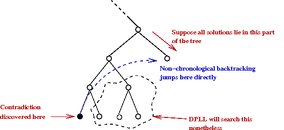
- DPLL backtracks one level "back".
- In many cases, DPLL wastes time exploring parts of the tree
where there's no solution at all
→
This is simply because DPLL works this way.
- In non-chronological backtracking, one can jump "back"
many levels.
- This idea was first used in AI searches by R.Stallman and
G.Sussman in 1977.
→
Yes, that Stallman.
- Idea #3: Use optimized data structures.
- It turns out a lot of time is spent in unit-clause propagation.
- Clauses have to be repeatedly checked to see if they
become unit clauses.
- Good data stuctures allow this to be done quickly.
- Idea #4: Perform several (randomized) re-starts.
- If one has spent too much time searching with no solution,
one can try a new random starting point (new order of variables).
- DPLL is known to be highly sensitive to the order of
variables searched in the exploration phase.
- Idea #5: In exploration phase, pick the next variable carefully.
- Idea #4 can be taken a step further.
→
Instead of selecting a random variable to explore, why not
a more promising variable?
- For example: pick the variable that most reduces the number
of unsatisfied clauses.
- Idea #6: Preprocess intelligently.
- Consider single-phase variables e.g., x3
only occurs as x'3 (in complemented form)
in the formula.
→
We can remove all clauses that contain a single-phase variable.
- Remove subsuming clauses, e.g., in
(x'3 + x7)
(x'3 + x7 + x9)
we can remove the second clause (since it will always be
satisfied if the first is satisfied.
- Idea #7: Combine all techniques into a "monster" (SATZilla) program.
Let's now look at conflicts and clause learning in more detail:
- We will use an example to illustrate some of the ideas.
- Suppose some large formula contains the following clauses
[some clauses] ....
(X'6 + X7)
(X1 + X'6 + X8)
(X'7 + X'8 + X9)
(X3 + X'9 + X10)
(X4 + X'9 + X11)
(X'10 + X'11)
(X6 + X12 + X'13)
(X10 + X11)
(X'2 + X'12 + X'14)
(X5 + X8)
... [other clauses]
- Next, suppose that exploration results in the following
variable assignments:
Exercise:
Simplify the clauses after these assignments. What remains?
Also, after the assignment X6=1, what other
assignments are forced?
- We'll use the term decision variable to
mean a variable whose value is assigned during exploration.
→
The other variables have their values forced by unit-clause propagation.
- Note: during the life of the algorithm a variable may
temporarily either type many times.
- The decision level d(v) of a variable v:
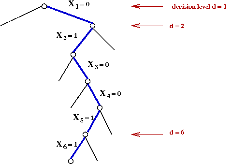
- d(v) = 1 if v is the highest-level decision variable
in the tree.
- d(v) = 1 + d(u) where u was the decision
variable assigned a value most recently prior to v's assignment.
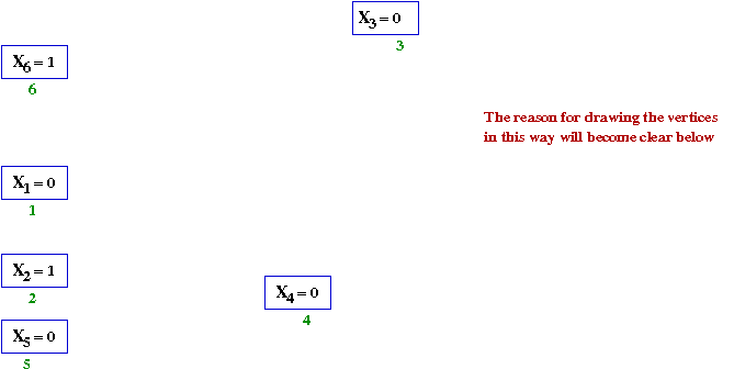
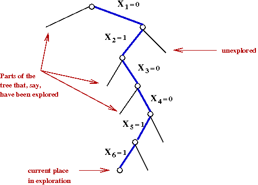
- Now, recall the sequence of decision assignments up through d=5:
      At d=1:    X1 ← 0
      At d=2:    X2 ← 1
      At d=3:    X3 ← 0
      At d=4:    X4 ← 0
      At d=5:    X5 ← 1
- After this, the clauses are:
(X'6 + X7)
(X'6 + X8)
(X'7 + X'8 + X9)
(X'9 + X10)
(X'9 + X11)
(X'10 + X'11)
(X6 + X12 + X'13)
(X10 + X11)
(X'12 + X'14)
- Setting X6=1 brings about the following chain of unit clauses:
      d=6:    X6 ← 1
      d=6:    This forces X7=1 and X8=1
      d=6:    This in turn forces X9=1
      d=6:    This forces X10=1
      d=6:    This forces both X11=1 and X11=0
              → A conflict!
- Note: we will associate the decision level of the forcing
variable (X6 in this case) with all the forced variables.
Next, we will build an associated directed graph called
an implication graph:
Key ideas:
- We build one such graph each time we get a conflict.
- The graph will be used to identify new clauses to add.
- The vertices are variable assignments, e.g. X6=1.
- A directed edge indicates when one variable forces the
assignment of another.
- We will first show the implication graph for the above
conflict and then explain how we produced the graph.
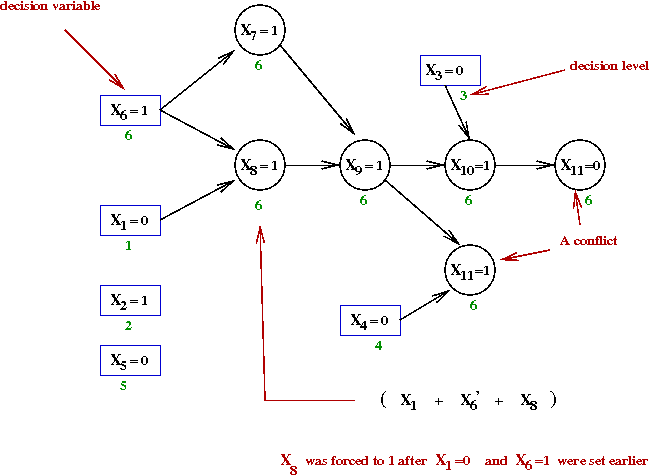
- There is a vertex for each variable assignment.
- Decision-variable vertices are in boxes, whereas the others
are in circles.
- Consider the node X8=1 above:
- This variable gets set to 1 because of the clause
(X1 + X'6 + X8)
- Here, X1=0 and X6=1
occured earlier.
→
This forces X8=1
- Anytime a variable's value is forced, we add edges from
the other variables that forced its value.
- Let's now see how the conflict graph was built step-by-step:
- Initially, there are 5 decisions that do not force assignments:
- Next, the variable X6←1
→
This forces X7←1 and X8←1
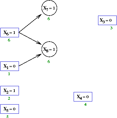
- Add variables X7←1 and X8←1.
- Examine the clause that forced X7←1
→
This is the clause (X'6 + X7)
- Add an edge from X6=1 to
X7←1.
- Similarly for X8←1 and the clause
(X1 + X'6 + X8),
→
Add the edges from X6=1 and X1=0.
- Next, the assignment X8←1 forces
X9←1 because of the clause
(X'7 + X'8 + X9)
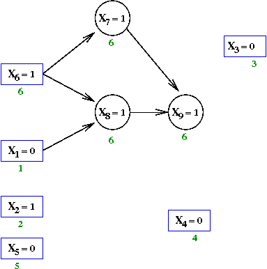
- Add edges from X7=1 and X8=1.
- Continuing, X9←1 forces X10←1.
and X11←1
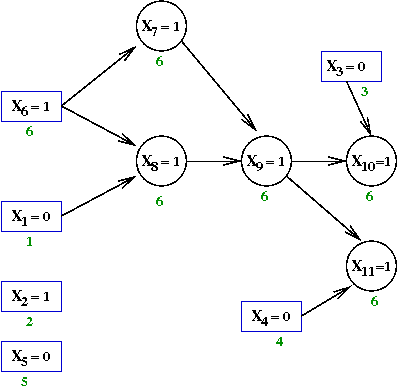
- Finally, X10←1 forces
X11←0
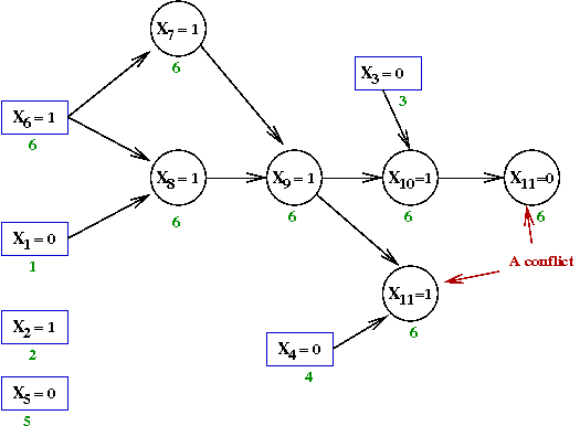
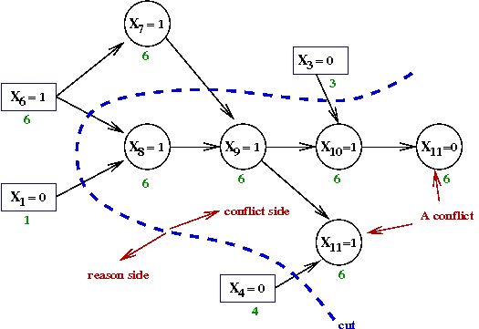
Next, what does one do with the implication graph?
- Clearly, from the graph, the decision variable assignments that caused the
conflict are
X1=0,
X3=0,
X4=0 and
X6=1
- Why? Because setting these values eventually leads to the conflict.
- If we are to avoid the conflict, at least one of these
variables must be set to its opposite value.
- For example, recall how X11 was forced
to the value 1 in the clause
(X4 + X'9 + X11)
- If instead of X4=0 we had X4=1
this would not occur.
- Consider the condition "at least one of the responsible decicion
variables must be oppositely set"
- In our case, the assignments were:
X1=0,
X3=0,
X4=0 and
X6=1
- The condition then becomes
X1=1 OR
X3=1 OR
X4=1 OR
X6=0
- We can write this as a clause!
(X1 + X3 + X4 + X'6)
- This clause can be added to the formula to force
this constraint to be satisfied.
- But, by adding a clause, did we change the problem? No, because:
- If the original formula is satisfiable, it could not be with
the implication-graph assignments
X1=0,
X3=0,
X4=0 and
X6=1
(because we know that this leads to a conflict).
- Thus, the new formula would also be satisfiable.
- Similarly, if the original formula is unsatisfiable,
(but the new clause is satisfiable), there must be
some other conflict.
- Notice that the implicated decision variables form a cut
of the graph:
- We could consider alternative cuts, such as:
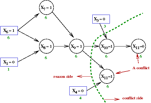
- This cut corresponds to the variable assignments
X3=0,
X4=0 and
X9=1.
- Thus, we could instead, alternatively, add the constraint
clause
(X3 + X4 + X'9)
- SAT algorithms differ in their choice of how to perform
cuts and which clauses (sometimes multiple) to add.
→
Experimental evidence is used to prefer one over another.
- So, when is the implication graph built?
- This too is an implementation choice.
- If we built implication-graph vertices as we go, we might
have too much work per iteration.
- If we build only when we detect a conflict, we will need
to examine the stack to re-construct the implication graph.
- For purposes of discussion, let's assume the graph is
built at the time a conflict is discovered.
Non-chronological backtracking:
Beyond DPLL, part II
We'll now examine some ideas related to:
- The choice of decision variable.
- Data structures.
Let's start with decision variables:
- At any time, if we have pushed through a chain of unit clauses,
we will have no unit clauses left
→
All remaining clauses are of size 2 or larger.
- This means, we need to pick a variable and set its value.
→
Continue exploration.
- Which variable to pick? DPLL picked a random one, but we
could be more clever in our choice.
- The MOMS (Maximum Occurrence in clauses of Minimum Size) heuristic:
- Identify all clauses of minimum size.
- Identify the variables in these clauses, including their phase.
- Pick the variable-phase combination that occurs most
frequently (breaking ties randomly).
- The intuition is that the solution is more sensitive to
variable-decisions in small clauses.
→
The most frequently occuring variable is likely to have the
largest effect, so try to pick this sooner.
- The DLIS (Dynamic Largest Individual Sum) heuristic:
- For a variable Xi, let
p(Xi) = # occurences of
Xi in remaining clauses.
q(Xi) = # occurences of
X'i in remaining clauses.
- Identify the variable Xm
that maximizes p(Xi) + q(Xi).
- Choose Xm as decision variable.
- If p(Xm) ≥ q(Xi)
set Xm=1, else set Xm=0.
- Intuition: try to pick the variable with the most effect
on number of affected clauses.
→
The goal is to reduce the formula as much as possible.
- The VSIDS (Variable State Independent Decaying Sum) heuristic:
- Initially, define p and q as above:
p(Xi) = # occurences of
Xi in remaining clauses.
q(Xi) = # occurences of
X'i in remaining clauses.
- But treat p and q as "scores" for each variable.
- Each time a conflict clause is added, increase the score
for the variables in the added clause.
- Periodically, re-scale or re-normalize to give preference
to the variables in the most recently added clauses.
- A variation (BerkMin solver): increase the scores of both
variables in the added clauses and variables in
the clauses that caused the conflict (in the edges of the "cut").
Next, let's examine data structures:
- Consider this example:
(X1 + X2)
(X'2 + X'3)
(X'2 + X4 + X6)
(X3 + X5)
(X3 + X6 + X7)
(X'2 + X6 + X7)
(X'2 + X3)
- Suppose we try X1=1:
- This results in a unit clause with X2
(X2)
(X'2 + X'3)
(X'2 + X4 + X6)
(X3 + X5)
(X3 + X6 + X7)
(X'2 + X6 + X7)
(X'2 + X3)
- Which in turn forces X2=1
(X'3)
(X4 + X6)
(X3 + X5)
(X3 + X6 + X7)
(X6 + X7)
(X3)
- Which results in a conflict.
→
And causes backtracking.
- When backtracking occurs, we need to un-do the assignmment
X1=1
→
And return to the starting set of clauses before the assignment.
- Unfortunately, this means un-doing the assignment in
many clauses, including non-unit clauses:
- For example, consider what happened when we assigned X2=1:
(X2)
(X'2 + X'3)
(X'2 + X4 + X6)
(X3 + X5)
(X3 + X6 + X7)
(X'2 + X6 + X7)
(X'2 + X3)
- X2 occurs in many clauses, some of which
are not unit clauses, and do not become unit clauses.
- Experiments show that a great deal of time is spent in
following chains of unit-clause propagations.
- Some of this is "useful"
→
Following the actual unit clauses.
- But some is merely making and un-doing assignments in
clauses that never become unit clauses.
- Consider a simple counter mechanism:
- Maintain two counters for each clause.
- CL = number of literals (size of clause)
- CF = number of literals that turned false.
- When CF = CL, the clause
is a conflict.
- When CF = CL-1, the clause
is a unit clause.
- Maintain pointers from each variable to the clauses in which
it occurs.
→
Separate lists for each phase of the variable.
- Every time a variable is set to a value, the appropriate
counters are updated.
- Every time an un-do occurs (backtrack), the counters are
again updated.
- In the watched-literals scheme, some of the un-do
work can be avoided:
[Mosk2001]:
- Key observation: as long as a clause has at least two
unassigned variables, it can't be a unit (or conflict) clause.
- For every clause that's not a unit clause:
maintain two literals whose values are unassigned.
- For every variable, maintain pointers to clauses where they
act as watched literals.
- When an un-do occurs, we don't have to worry about
clauses where the variable is not a watched literal.
- Example: consider setting X2=1:
(X2)
(X'2 + X'3)
(X'2 + X4 + X6)
(X3 + X5)
(X3 + X6 + X7)
(X'2 + X6 + X7)
(X'2 + X3)
- Suppose that the two larger clauses have
(X4, X6),
and (X6, X7)
as watched literals.
- Here, we need to un-do the status of the small clauses in which
X2 occurs.
- But the two larger clauses have other variables that are unassigned.
→
There's no need to explicitly un-do anything in those clauses.
How are all these ideas worked into DPLL?
Summary
The Satisfiability (SAT) problem is one of the most important problems
in computer science:
- SAT is the foundational problem in the theory of NP-completeness
and problem complexity.
- SAT is a building block of algorithms in logic:
- Algorithms for automated theorem proving.
- Algorithms for model checking and program correctness.
- SAT has many applications just by itself:
- Logic design, circuit testing.
- Planning, knowledge representation.
- Example of a new application: cryptanalysis
- Consider encryption using some well-known algorithm such as AES:
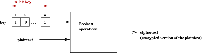
- When the key is not known but plain-cipher combinations (cribs)
are known, we can model the result as a Boolean expression:
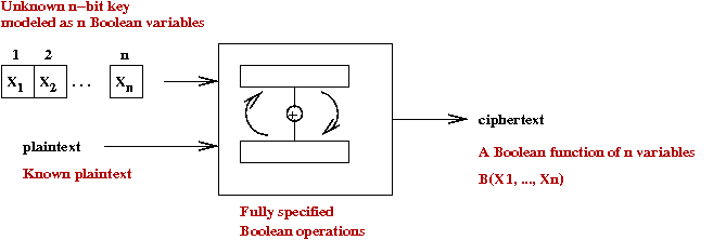
- This can be converted to CNF.
- Then, we can ask: is the Boolean expression satisfiable?
- One of the solutions will be a key
→
Which can greatly reduce the search space for keys.
- More generally, such analysis can help identify weaknesses
in ciphers.
What we learned about SAT solvers:
- The original DPLL algorithm is still the main idea.
- A combination of clever modifications has a dramatic effect
→
From a few hundred variables to millions of variables.
- There is a biannual (every two years) SAT competition.
See the SAT competition page.
- Many of the ideas we have studied have come from the winners.
References and further reading
[WP-1]
Wikipedia entry on SAT.
[Sat-comp]
SAT competition page.
[Aspv1979]
B.Aspvall, M.F.Plass and R.E.Tarjan
A linear-time algorithm for testing the truth of certain
quantified boolean formulas.
Inf. Proc. Lett, 8:3, 1979, pp.121�V123.
[Auda2009]
The
Glucose solver. See
Predicting learnt clauses quality in modern SAT solvers.
IJCAI, 2009, pp.399-404.
[Bier2010]
A.Biere et al.
The PrecoSAT project website.
See also:
M.Jarvisalo, A.Biere, and M.Heule.
Blocked Clause Elimination,
TACAS, 2010.
[Davi1960]
M.Davis and H.Putnam.
A computing procedure for quantification theory.
J.ACM, 7:3, 1960, pp.201-215.
[Davi1962]
M.Davis, G.Logemann and D.Loveland.
A machine program for theorem proving.
Comm. ACM, 5:7, 1962, pp.394-397.
[Dubo2001]
O.Dubois and G.Dequen.
A backbone-search heuristic for efficient solving of hard 3-SAT formulae.
IJCAI, 2001.
[Een2003]
N.Een and N.Sorensson.
An extensible SAT solver.
SAT, 2003.
See the MiniSAT and SatELite website.
[Gebs2007]
M.Gebser, B.Kaufmann, A.Neumann, and T.Schaub.
CLASP: A Conflict-Driven Answer Set Solver,
LPNMR,
2007, pp.260-265.
See the Clasp project website.
[Gent1993]
I.P.Gent and T.Walsh.
Towards an Understanding of Hill-climbing Procedures for SAT.
AAAI, 1993, pp.28-33.
[Gome2008]
C.P.Gomes, H.Kautz, A.Sabharwal and B.Selman.
Satisfiability Solvers.
Chapter 2, Handbook of Knowledge Representation,
Elsevier 2008.
[Gu1997]
J.Gu, P.W.Purdom, J.Franco and B.Wah
Algorithms for the Satisfiability (SAT) Problem: A Survey.
In: "Satisfiability Problem: Theory and Applications",
DIMACS Series in Discrete Mathematics and Theoretical
Computer Science, American Mathematical Society, pp. 19-152, 1997.
[Li2005]
C.M.Li and W.Huang.
Diversification and Determinism in Local search
for Satisfiability,
SAT2005, St Andrews, UK, June 2005, Pages 158-172.
See the TNM Solver website.
[Marq1999]
J.Marques-Silva and K.A.Sakallah.
GRASP: A search algorithm for propositional satisfiability.
IEEE Trans. Comput., 48:5, 1999, pp.506-521.
[Marq2008]
J.Marques-Silva.
Practical Applications of Boolean Satisfiability.
In: Workshop on Discrete Event Systems (WODES'08),
May 2008, Goteborg, Sweden.
[McAl1997]
D.McAllester, B.Selman, and H.Kautz.
Evidence for Invariants in Local Search
Proc. AAAI-97, Providence, RI, 1997.
[Mitc2005]
D.G.Mitchell.
A SAT Solver Primer.
EATCS Bulletin (The Logic in Computer Science Column),
Vol.85, February 2005, pages 112-133.
[Mona1999]
R.Monasson, R.Zecchina, S.Kirkpatrick, B.Selman and L.Troyansky.
Determining computational complexity from characteristic `phase transitions'.
Nature, Vol. 400(8), 1999, pp.133--137.
[Mosk2001]
M.Moskewicz, C.Madigan, Y.Zhao, L.Zhang and S.Malik.
Chaff: Engineering an Efficient SAT Solver.
39th Design Automation Conference (DAC 2001),
Las Vegas, June 2001.
See the Chaff project website.
[Nude2004]
E.Nudelman, A.Devkar, Y.Shoham , K.Leyton-Brown and H.Hoos.
SATzilla: An Algorithm Portfolio for SAT.
Int.Conf. Theory and App. of SAT, 2004.
See also the
project website.
[Pipa2008]
K.Pipatsrisawat and A.Darwiche
A New Clause Learning Scheme for Efficient Unsatisfiability Proofs.
AAAI, 2008.
See the RSat project website.
[Selm1992]
B.Selman, H.Levesque and D.Mitchell.
A New Method for Solving Hard Satisfiability Problems.
AAAI, 1992, pp.440-446.
[Selm1995]
B.Selman, H.Kautz and B.Cohen.
Algorithms for the Satisfiability (SAT) Problem: A Survey.
DIMACS Series in Discrete Mathematics and Theoretical
Computer Science, American Mathematical Society, pp.521-532, 1995.
[Will2003]
R.Williams, C.Gomes and B.Selman.
Backdoors To Typical Case Complexity.
Proc. IJCAI-03, Acapulco, Mexico, 2003.
[Zhan2003]
L.Zhang.
Searching for truth: techniques for satisfiability of
Boolean formulas.
PhD thesis, Princeton University, 2003.
See also his
set of slides.