Note: Shannon used the mathematical formulation of minimax
for game theory
→
From Von Neuman and Morgenstern
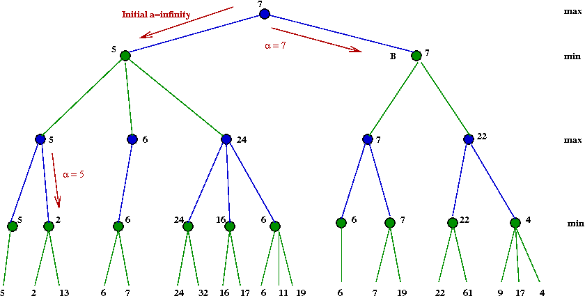
Exercise:
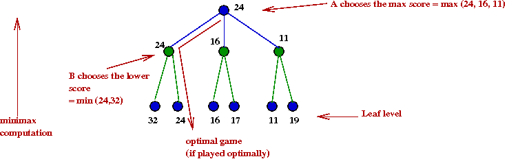
Apply the minimax algorithm to this game tree:
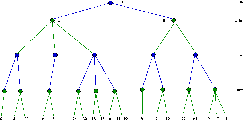
Do all subtrees need to be explored?
- Consider this example with part of the tree explored:
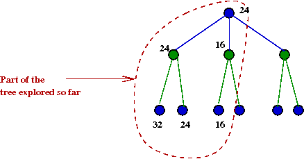
- Suppose we knew the max-value A=24
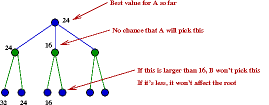
- After we have explored the B=24 node, we
next explore the B=16 node.
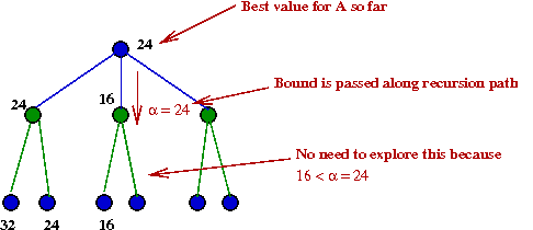
- There is no need to explore the right child of B=16.
→
Because this is already lower than α=24
- Suppose we recorded the "best so far" during execution
- The alpha-beta algorithm:
     Algorithm: findMax (state, α, β)
     Input: the current "board" or state
     1.   if state is terminal
     2.      return (null, value(state))
     3.   endif

          // Search recursively among child states
     4.   M = generate all possible moves
     5.   maxValue = -∞
     6.   for m ε M
     7.      s = state (m)                // s is the state you get when applying move m
     8.      (m',v) = findMin (s, α, β)   // m' is the best min move
     9.      if v > maxValue
     10.        maxValue = v
     11.        bestMove = m
     12.     endif
             // If we've exceeded some earlier B's min-value, there's no point searching further in this A-node's children.
     13.     if maxValue ≥ β
     14.        return (bestMove, maxValue)
     15.     endif
             // Update this node's best value so far.
     16.     if maxValue > α
     17.        α = maxValue
     18.     endif
     19.  endfor
     20.  return (bestMove, maxValue)
     Algorithm: findMin (state, α, β)
     Input: the current "board" or state
     1.   if state is terminal
     2.      return (null, value(state))
     3.   endif

          // Search recursively among child states
     4.   M = generate all possible moves
     5.   minValue = ∞
     6.   for m ε M
     7.      s = state (m)                // s is the state you get when applying move m
     8.      (m',v) = findMax (s, α, β)   // m' is the best max move
     9.      if v > maxValue
     10.        minValue = v
     11.        bestMove = m
     12.     endif
             // If we've exceeded some earlier A's max-value, there's no point searching further in this B-node's children.
     13.     if minValue ≤ α
     14.        return (bestMove, minValue)
     15.     endif
             // Update this node's best value so far.
     16.     if minValue < β
     17.        β = minValue
     18.     endif
     19.  endfor
     20.  return (bestMove, minValue)
Exercise:
Use the example in the previous exercise and work out
the steps in the α-β algorithm.
- Note:
Exercise:
Modify the Minimax code to implement α-β pruning
and test it out with tic-tac-toe.
Iterative deepening:
- An idea that's been around since the early days of search.
- How it works:
- Start with max-depth d=1 and apply full search to this depth.
- Make d=2, and search.
- Increment d, repeat.
- Let's take this a step further by writing it in pseudocode:
     Algorithm: Iterative-Deepening (search, maxTime)
     Input: a search algorithm, and a time limit.
     1.   d = 1
     2.   while currentTime < maxTime
     3.      m = search (d)              // Apply search algorithm, e.g., α-β, to depth d
     4.      d = d + 1
     5.   endwhile
     6.   return m                       // Best move found so far
- Wait a minute - why waste time doing the first few iterations?
- One has limited time in games
→
This way, one has a "best" move at some depth d.
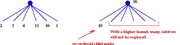
- More importantly, one can re-order the root's children
based on previous depth
→
Makes α-β more effective.
     Algorithm: Iterative-Deepening (search, maxTime)
     Input: a search algorithm, and a time limit.
     1.   d = 1
     2.   while currentTime < maxTime
     3.      m = α-β-search (d)              // Apply search algorithm, e.g., α-β, to depth d
     4.      re-order children of root.
     5.      d = d + 1
     6.   endwhile
     7.   return m                           // Best move found so far
- Also, with each iteration, the transpostion table adds positions
→
These won't be searched.
The chess tree:
- Average of 35 possible moves per position (average branching factor).
- For a 50-move (100-ply) game
→
35100 nodes (approx. 10154) in tree.
- Note: an endgame might have as few as 4-6 pieces
→
These game trees can be explored off-line (and have been).
Back to Shannon:
- Shannon realized that a full exploration is not possible.
- Instead of going down to a leaf-level, stop at some depth.
- Use a scoring function to evaluate positions at max-depth.
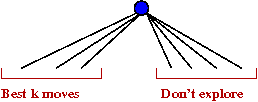
- Two types of search:
- Type-A: fix a depth and do a complete search of tree until that depth.
- Type-B: explore some promising moves more deeply than others.
- Shannon's scoring function:
- Material points: Q=9, R=5, B=K=3, P=1, K=200.
- Pawn structure: penalty of 0.5 for each doubled or isolated pawn.
- Piece-mobility: 0.1 points per possible move per piece.
He also recommended other scoring attributes.
- Note: score granularity = 0.1.
- For comparison: Deep Blue's scoring function
- Much smaller granularity.
- 8000 different contributing factors.
- Searching:
- Shannon used minimax (depth-first) search.
- Because recursion was not supported then, an elaborate
data structure was used to track the state and the current position in the (implied) tree.
- Shannon never got around to implementing his (seminal) ideas.
The first decade: Kotok and Kaissa
Newell, Shaw and Simon:
- All pioneers in AI.
- Devised a programming language called IPL for problem-solving
tasks.
- IPL was used to build NSS in 1955, a type-B chess program.
→
Did not perform well at all.
- Historical side note: Newell spent many years working
with J.B.Kruskal (of MST fame) on optimization problems.
MIT vs. ITEP
- MIT:
- Alan Kotok, a student of AI pioneer John McCarthy at MIT.
- Type-B program, 4-ply search depth.
- In Fortran, on an IBM 7090.
-
- The Institute of Theoretical and Experimental Physics (ITEP)
in Moscow:
- Team leader: George Adelson-Velsky (the "AV" of AVL).
- Main programmer: Vladimir Arlazarov.
- Type-A program.
- 5-ply search depth
- First ever computer-computer match in 1966:
→
ITEP won 3-1.
- A foreshadowing of the intellectual battle within
computer chess:
→
Type-A vs. Type-B.
- Kaissa:
- Mikhail Donskoy was added to the ITEP group.
- New program was called Kaissa.
- Ran on a British ICL 4/70.
- Used "board similarity" to avoid evaluating some nodes.
- Dominated computer chess until 1976.
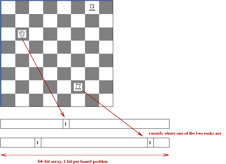
- Kaissa introduced a useful data structure: the bitboard:
- One obvious way to store a chessboard: 8 x 8 array of pieces.
- A less obvious way: the bitboard
- A side note about the IBM 7090:
- Among the first of second generation (transistor) machines.
- Cost: $2-3 million.
- Was used for CTSS (first time-sharing OS) at MIT.
The second decade: MacHack and Chess 4.5
MacHack:
- Written by Richard Greenblatt:
- One of the legendary first generation of "hackers"
- Main programmer for Lisp and various other projects out of MIT.
- First version in 1966:
- On a PDP-6 (cost: $400,000).
- In assembly.
- Type-B strategy.
- 4-ply search depth.
- Other features added:
- First program to use an opening book
→
Stored opening moves.
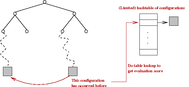
- First program to use a transposition table
→
Essentially a hash table storing previously-scored positions.
- Performance:
- Never played against other programs (Greenblatt's bias).
- Played against humans in local competitions
→
Received a chess rating of 1510 (modest).
- Lost badly to Bobby Fischer, then a rising star.
- Won against some class-A players
→
Achieved a rating of 2271, highest ever for a program in 1978.
Chess 4.5 history:
- Started as Chess 2.0 in 1968 by Larry Atkin, David Slate and others
at Northwestern University.
- Grew into Chess 3.0, 3.6, etc until 4.5.
- Type-B strategy until 3.6, then type-A.
- Won the first ACM Computer Chess Championship in 1970,
and many others in the 1970's.
- Played well against humans, e.g., won 5-0 in
class-B (rating below 1800) of the Paul Masson Chess Championship
in 1976.
Type-A vs. Type-B:
- In early programs, type-A was thought to be a waste
of time
→
Better to search only promising moves in greater depth.
- A type-B program spends much of its time sorting
moves:
- A sophisticated evaluation function is time-consuming.
- A minimax type-A program only evaluates positions at
at the leaf level.
→
Simple minimax for interior nodes.
- A type-B program evaluates all interior nodes (even if
it has fewer).
- However, a type-A that sorts its interior nodes
(for better α-β) will also do evaluation
→
But this can be a much simpler evaluation (because it
doesn't affect quality, only speed).
Chess 4.5 technical details:
- Earlier versions were a mix of Fortran and assembly.
- Chess 4.5 was entirely in CDC 6000 assembly.
- A database of bitboards:
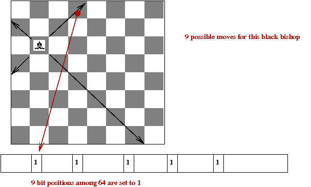
- One bitboard per major piece for every possible location.
→
All possible moves for that piece.
- Bitboards use bit-operations
→
e.g., remove all "friendly" positions from bishop-bitboard.
- Quiescent search:
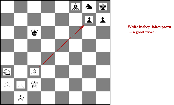
- Above, when White plays B x p, it looks like
a poor move
→
Will lead to a low evaluation score.
- But it does lead to a queen capture when followed through.
- Quiescient search follows captures and checks
depth-first until they end, even if they violate depth-limit.
- A sophisticated evaluation function:
- Material balance.
- Pinned pieces (pieces under attack from others).
- Pawn structure.
- Mobility and "center" control.
- Special rules for each piece, e.g., open files available to rooks.
- Three different hash tables:
- Transposition table.
- Material balance table
→
Stores only which-pieces-are-active, for quick material balance computation (by lookup).
- Pawn structure hash table.
→
To take pawn structure as input and output an evaluation score.
- Killer-move table:
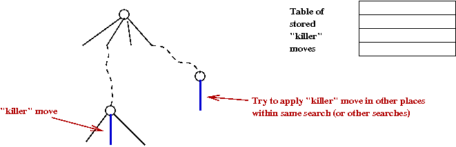
- Moves that are very good are saved to see if they can
be applied later:
- Also called a refutation move.
- Search strategy:
- See if position is in opening book, and if so,
try to follow opening book.
- If not, start with 2-ply iterative deepening.
- Successively add one ply at a time to iterative deepening.
- Look up each generated position in transposition table
to see if it has been scored.
- Apply all the other tricks (killer moves etc).
The Levy challenge and Fredkin Prize
Challenges issued to chess programmers:
- David Levy, a chess Master:
- 1968: he bet $10,000 that
no program would defeat him in the decade 1968-78.
- He played a variety of programs, including Chess 4.5 until 1977
→
Won all his games.
- In 1978, he played Chess 4.7
→
He won the match but lost one game and drew the other.
- In 1989, he lost to Deep Thought (the precursor to Deep Blue).
- He predicted that Kasparov would win 6-0 against Deep Blue.
- Levy is the author of Love and Sex with Robots.
- Edward Fredkin, entrepreneur, scientist and professor (at MIT).
- The first programmer of the PDP-1.
- A director of Project MAC at MIT.
- Inventor of the trie data structure.
- Various other odd and interesting contributions.
- Fredkin Prize:
- Established in 1980.
- $100,000 to the first program that defeats the world champion.
- Intermediate prizes ($5,000 and $10,000) to achieve Master
and Grandmaster status.
- 1983: First intermediate prize won by Belle (see next section).
- 1988: Second intermediate prize won by Deep Thought (precursor to
Deep Blue).
- Grand prize won by Deep Blue after defeating Kasparov in 1997.
Belle
An overview:
- Built by Ken Thompson (of Unix/C fame) and Joe Condon at AT&T Bell labs.
- Started as software in 1973, using type-A.
- In 1976:
- A small move-generator built in hardware to use as
a supplement to the PDP-11 running the software.
- Software completely re-written in the style of Chess 4.5.
- Performed poorly in 1977 Computer Chess Championship.
→
Hardware slowed the software.
- Interesting aside: in the 1977 Championship,
an estimated $40 million worth of computers were being used
by contestants.
- In 1978:
- Second generation Belle.
- Search speed: 5000 positions/second.
- Main software: α-β on PDP-11, supplemented
by hardware move-generator.
- Won the 1978 ACM Computer Chess Championship.
- In 1980:
- Third generation Belle.
- More functionality in hardware: move generation, evaluation,
transposition memory, and parts of search.
- Average of 150,000 positions/second.
- Average 8-ply search, with occasional increases on
quiescent moves or endgames.
- Software opening book with 360,000 positions.
- End-game databases with all possible 3,4 and 5-piece
combinations.
- Belle's performance
- Won most competitions in early 1980's.
- Achieved a chess rating of 2363.
- Was awarded the first Fredkin Intermediate prize in 1983.
- Lost to Cray Blitz (highly parallel search) soon after.
More about Belle:
- First, consider the difficulty of software move-generation:
- First you have to locate your pieces in the data structure.
- Then, you need to identify where each piece can move
→
called pseudo-legal moves (without taking "king check" into account).
- Then, if you are ordering moves for α-β you need
at least some cursory evaluation.
- This can be sped up with bitboards, but it is still time consuming.
- Belle and Deep Blue use special purpose hardware with
the following general idea:
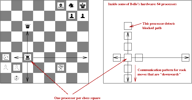
- Each chessboard square is represented with a circuit unit.
- There are control lines such that each unit can communicate
with its (at most 8) neighbors.
- Signals go back and forth in parallel.
- Each piece can determine where it can move (in parallel with others).
- The circuitry is highly optimized so that many circuit events
take place in a single cycle of the main processor.
→
e.g., in Belle, all possible moves for piece are detected in a single cycle.
- Belle also performed other functions in hardware:
- A 64-unit evaluation component
→
Similar in architecture to the move-generator, but to evaluate a position in parallel.
- 1-megabyte memory board to store the transposition table,
along with a fast hardware-computed hash.
- A separate processor for the α-β algorithm.
- 30MB of storage (phenomenal in those days) for databases.
Finally, an interesting study using Belle:
- With Chess 4.5 and Belle, computer chess programs started
to receive chess ratings.
- What is a chess rating?
- A complicated scoring system that is based on your
games with other (rated) players.
- Scores above 2000: expert-level and higher.
- Garry Kasparov: at 2851, the highest rated chess player ever.
- Thompson asked: what is the increase in rating for a given
increase in speed or search depth?
- He played various versions of Belle against itself (with different search depths)
→
Approx. an increase in 250 points for every additional level of depth.
Deep Blue
Recall type-A vs. type-B:
- Even though type-B programs got more sophisticated,
the majority of wins were from type-A programs.
- However, this issue was not yet settled with the next
generation: mid-80's to 90's.
- A mostly-friendly rivalry of the two types emerged
at CMU:
- HiTech - a parallel-machine implementation of
a sophisticated type-B strategy, led by Hans Berliner (himself
a chess champion).
- ChipTest - a hardware implementation of the
basic type-A strategy.
- ChipTest and HiTech did reasonably well, and each grew
in stature.
- ChipTest:
- ChipTest was led by Feng-Hsiung Hsu, a graduate student CMU.
- Other contributors: Thomas Ananthraman,
Andreas Nowatzyk, Murray Campbell.
- Later version of ChipTest would achieve 500,000 positions/second.
- Deep Thought:
- Evolved from ChipTest.
- Basically: more and better hardware.
- Parts of the software were re-written.
- Included a bigger opening book.
- Routinely achieved 1,216,000 positions/second in search speed.
→
200 million or more positions per move.
- Deep Thought's performance:
- At this point, the only interesting opponents were humans.
- 1989: it beat David Levy (recall: Levy's bet).
- 1989: Drew with Robert Byrne, a grandmaster.
- 1989: lost to Kasparov.
- 1989: lost to Karpov.
Deep Blue:
- The Deep Thought team moved to IBM (Campbell and Hsu) and
acquired Joe Hoane as principal programmer.
- The project name became, naturally, Deep Blue.
- First historic match with Kasparov in 1996:
- 32-node IBM RS/6000 cluster as the main computer.
- 192 specialized VLSI chess processors based on the
Deep Thought hardware architecture.
- Up to 100 billion positions searched per move.
- Kasparov won 4-2, but received a shock by losing the first game.
- Second historic match with Kasparov in 1997:
- An upgraded (faster) 30-node cluster.
- 480 chess processors, each able to search 2.5 million positions/second.
→
An average of 126 million positions per second in practice.
- At least 6-8 ply per move, average of 10-12 ply,
sometimes as much as 20-ply.
- 4000 openings and 700,000 stored grandmaster-level games.
- Fine-tuning of parameters based on playing against
grandmaster Joel Benjamin.
- Deep Blue defeated Kasparov 3.5-2.5, winning the Fredkin Prize.
More about Deep Blue's internals:
- Evaluation function with 8000 features:
- Dynamic: changes during the course of the game.
- Tunable parameters - based on games played against
grandmasters and against Kasparov's previous games.
- Opening book:
- 4000 openings created by hand by grandmaster Joel Benjamin.
- Each opening explored with long, independent runs on Deep Blue.
- Database of 700,000 grandmaster games:
- To be used to evaluate positions
→
"If a grandmaster made this move, it must be good".
- The results were weighted by a number of factors:
Kasparov's own moves, comments by better grandmaster etc.
- Endgame database:
- All endgames with 5 pieces or fewer.
- Many 6-piece endgames.
- Stored on 20GB of additional storage.
- Software/hardware division of search functionality:
- Most searching was performed in hardware.
- But some specialized moves (e.g, forced or quiescent sequences)
were performed in software.
- First two plies always in software, which then distributed
control of further searches to hardware.
- Sophisticated parallelism:
- By now, parallel computation issues in search were well understood:
→
When to load-balance, when to communicate between processors etc.
Postscript:
- The 1997 historic event did not end as happily:
- Kasparov asked for a re-match but IBM refused.
- Hsu acquired rights and tried to acquire private funding
to continue, but was not successful.
- Many criticized IBM for not being more open about its decisions.
- Today, Deep Blue's power is being achieved by all-software
desktop programs:
- For example, in 2006, Deep Fritz defeated world champion Victor Kramnik.
- Rybka is the current (2006-09) computer chess champion.
Checkers and Chinook
About Chinook:
[Scha1992].
- A program developed by Jonathan Schaeffer and others to
play checkers.
- In chess, the human opponent (Kasparov) was considered
one of the best players of all time.
- In checkers, there was no doubting the ability of
the human opponent, Prof. Marion Tinsley:
- Math prof at Florida State University.
- Perhaps the most remarkable board game player ever.
- World champion 1955-58, and 1975-91.
- Never lost a championship (he retired 1959-1974).
- Lost only 7 games in his entire 45-year career!
→
Two of them to Chinook.
- Claimed he could "see 50 moves ahead."
- Against Chinook:
- Tinsley beat Chinook 4-2 in 1992.
- In 1994, after six draws with Chinook, Tinsley withdrew for health reasons (he died later than year).
Chinook technical details:
- Just like Deep Blue and others:
- A highly parallelized heuristic search: α-β.
- A database of openings and endgames.
- A complex evaluation function.
- Hardware:
- Standard workstations.
- In 1994: 16 150MHz Silicon Graphics processors.
- Search:
- Average search depth of 19 ply.
- Many rules specialized to certain key moves in checkers.
→
Many cases of quiescent search.
- Example: a scenario called two-for-one (sacrifice followed by a two-piece capture).
→
8,000,000 such pre-stored positions.
- Evaluation function:
- 24 different factors.
- Carefully hand-tuned.
- Endgame database:
- All endgames for 8 or fewer pieces.
- 440 billion positions, compressed into 6 GB.
- Openings:
- 144 3-ply openings.
- All non-standard openings were deeply analyzed (to try and
surprise Tinsley).
The more important result about Chinook:
[Scha2007].
- In 2007, Schaeffer and colleagues presented evidence that
"checkers is solved"
→
That Chinook could do no worse than draw against anyone.
- To prove this, they ran an astronomical number of games
in an organized way.
- First, they solved all 10-piece end games completely.
- Approx. 4 x 10¹³ positions.
- Compressed into 237 GB, with a specially designed compression algorithm.
- They reduced the possibilities after the first 3-ply to 19
configurations
→
Using symmetry arguments.
- Each of these 19 configurations was explored using minimax
until a 10-piece "draw or better" configuration was achieved.
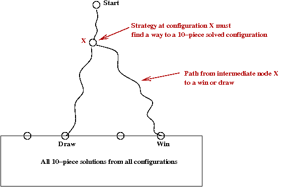
- Many clever heuristics to avoid searching all of the space.
- Goal was only to show it could be done, not to actually
store the winning move sequences.
- Large parallel machine infrastructure with load balancer
to efficiently manage the search.
- One of the most intensive computations of all time.
What does it all mean?
Here are two interesting questions:
- Why did MPBF ("Massively Parallel Brute-Force") win
over more clever, refined heuristics?
- Can MPBF be called "intelligent"?
Exercise:
What do you think?
On the first question:
- One response is that the success of MPBF reflects
the nature of chess or checkers.
→
Even seemingly poor moves need to be explored at sufficient depth.
- On the other hand:
- If it were true that low-depth positions could be successfully
evaluated, humans would have discovered this
→
It would be boring, like tic-tac-toe.
- Complex games are interesting because they stratify humans
(weak to grandmaster).
→
One is in awe of the effort needed to become a grandmaster.
- MPBF appears to be succeeding in other AI fronts
→
e.g., pattern recognition, NLP.
On the second question:
- Recall the Chinese room argument. Is the room intelligent?
- Should a Turing-like test be sufficient to determine
intelligence?
- Should consciousness count?
Finally, a humorous comment:
Chess is the Drosophila of artificial
intelligence. However, computer chess has
developed much as genetics might have if
the geneticists had concentrated their efforts
starting in 1910 on breeding racing
Drosophila. We would have some science,
but mainly we would have very fast fruit
flies.
-- John McCarthy
References and further reading
[WP-1]
Wikipedia entry on chess programs.
[WP-1]
Computer Museum website on chess.
[Camp1999]
M.Campbell. Knowledge discovery in Deep Blue.
Comm. ACM, 42:11, 1999, pp.65-67.
[Camp2002]
M.Campbell, A.J.Hoane and F-H.Hsu.
Deep Blue. Artificial Intelligence, Vol.134,
2002, pp.57-83.
[Frey1983]
P.W.Frey (editor),
Chess Skill in Man and Machine,
Springer, 1983.
[Hsu1999]
F-H.Hsu. IBM's Deep Blue chess grandmaster chips.
IEEE Micro, March-April, 1999, pp.70-81.
[Hsu2002]
F-H.Hsu. Behind Deep Blue,
Princeton University Press, 2002.
[Newb1997]
M.Newborn. Kasparov vs. Deep Blue: Computer
Chess Comes of Age, Springer, 1997.
[Russ2003]
S.Russell and P.Norvig.
Artificial Intelligence: A Modern Approach (2nd Ed),
Prentice-Hall, 2003.
[Scha1992]
J.Schaeffer, J.Culberson, N.Treloar, B.Knight, P.Lu and D.Szafron.
A World Championship Caliber Checkers Program.
Artificial Intelligence, Vol.53, No.2-3, 1992, pp.273-290.
[Scha2007]
J.Schaeffer, N.Burch, Y.Bjornsson, A.Kishimoto, M.Muller,
R.Lake, P.Lu and S.Sutphen.
Checkers is solved.
Science, Vol.317, Sept 2007, pp.1518-22.