Matches, Recommendations and the Netflix Challenge
Overview
A preview:
- An abstract marketplace: matching users to items.
- The stable marriage problem.
- Graph matching.
- Text matching (mining).
- Data mining.
- Collaborative filtering.
Our presentation will pull together material from various sources - see the
references below. But most of it will come from
[Bree1998],
[Grif2000],
[Herl1999],
[Roth2008],
and
[Su2009].
Matching users to items: the marketplace
Consider an abstract market:
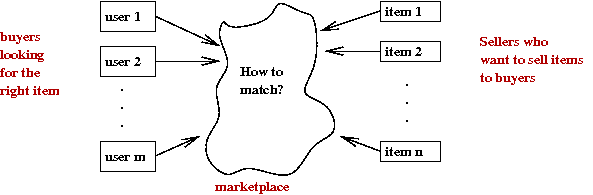
- There are a number of users.
- And a number of items or "goods".
- Each user (buyer) is looking for some items.
- Sellers both want to match their items with buyers
and also want to promote new items.
The standard approach: a supply-demand marketplace with prices
- Assume items are priced by sellers.
- Users have knowledge of all items and prices.
- Users optimize some "utility" function that takes
into account items and prices.
- Users purchase items.
Market failures:
- Unfortunately, standard markets can fail spectacularly in
many cases.
- Example: college admissions
- Here, users = students and items = college-seats.
- Prices are known ahead of time.
- But items are limited, with one copy per buyer
→
a challenge for buyers
- Also, all items must be sold
→
a challenge for sellers
- Yet, both buyers and sellers compete.
- In limited resource regime:
- Some other arrangement than a free-market is used.
- But that has its own problems.
- Problem #1: unraveling
- A "competition" of early offers.
→
race to the bottom by sellers.
- Early offers with buyer-commitment
→
not the best choice for buyers.
- Problem #2: congestion
- When a seller learns that a buyer declined, it must
rapidly contact "second ranked" buyers.
- And "second ranked" buyers have little time to decide.
- Problem #3: deception
- Both buyers and sellers are encouraged to be deceptive
→
Doesn't pay to reveal your preferences.
- Example: if college X knows that a student's top choice is college Y, it doesn't help the student.
→
Student is pressured to conceal this fact.
- Other types of market failures:
- Buyers are sometimes unable to find "best-match" items.
- Buyers sometimes don't know of the existence of items
that they would like.
- Sellers unable to discern what a buyer is actually looking for.
Let's examine an abstract market along two dimensions:
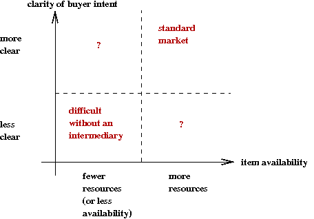
- The first dimension: resources
- In some markets, the resources, and therefore items, are limited.
- Examples: college seats, airline seats, auctions.
- The second dimension: clarity of buyer intent
- Buyers aren't able to exactly state what they want.
- Buyers aren't aware of items they may need or want.
- Now, let's examine the four cases.
- High-resource and high-clarity.
- Low-resource and low-clarity.
- Low-resource and high-clarity.
- High-resource and low-clarity.
- Case 1: High-resource and high-clarity.
- This is the standard market.
- Buyers shop around for best prices or deals.
- Sellers compete on price, on branding, on deals etc.
- Example: books.
- Case 2: Low-resource and low-clarity.
- Buyers aren't sure of what exactly they're looking for.
- Sellers have limited items.
- Most often, an intermediary is helpful
→
Creates a market for intermediaries.
- Example: real estate.
- Case 3: Low-resource and high-clarity.
- College admissions example.
- Case 4: High-resource and low-clarity.
- Buyers aren't looking for a particular item, but some
vaguely stated "category".
- Sellers want to stimulate buyer interest and try to match
buyers with items.
- Example: idle browsing for movies, songs.
- Cases 1 and 2 are uninteresting from our point of view.
- Our focus: cases 3 and 4:
- Case 3: Algorithms for matching.
- Case 4: Algorithms for helping sellers recommend items to buyers.
The stable marriage problem
First, let's describe the problem:
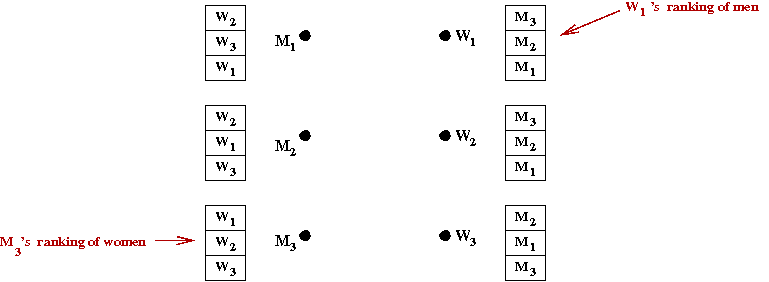
- We will describe the simplest version of the problem:
- n men: M1, M2, ..., Mn.
- n women: W1, W2, ..., Wn.
- Each man lists all women in some order of preference.
- Each woman lists all men in some order of preference.
- Broad goal: pair each man with a woman.
- Thus, there is perfect clarity in buyer intentions, but limited resources
→
Each man is paired with one woman in the pairing.
- We'll use the notation (Mi,Wj) to denote a couple produced by a pairing or marriage.
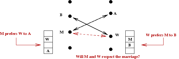
- A marriage is stable if there is no
Mi and Wj such that:
- Mi and Wj are not married.
- Mi is higher in Wj's list
than her current spouse.
- Wj is higher in Mi's list
than his current spouse.
- This is important because otherwise,
Mi and Wj
would not respect the marriage and would elope.
- Example: the marriage below is not stable:
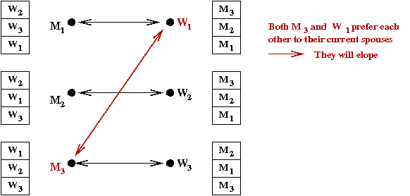
- Thus, our goal is: compute a stable marriage if one exists.
The Proposal Algorithm:
- Due to David Gale and Lloyd Shapely in 1962
[Gale1962].
- Also called the Deferred-Acceptance Algorithm.
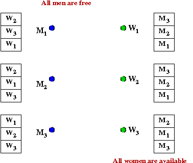
- Key ideas: "man proposes, woman disposes"
- Initially, all men and women are "free".
- At each step, there is an engagement.
- At each step, a free man proposes to any woman who
has not rejected him before.
- A woman is required to accept unless she's engaged
to someone higher on her list.
- If a woman is engaged to a lower-preference man,
she "dumps" that man in favor of the proposer.
- After no more engagements are broken and all are engaged,
the marriage is finalized.
- Note: the women always "trade up".
- Let's work through an example:
- M1 proposes to W2
→
She accepts
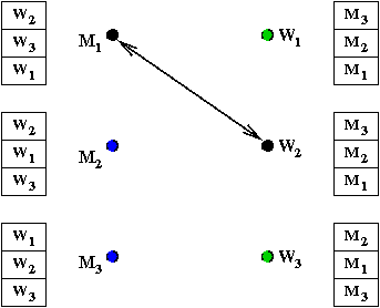
- M2 proposes to W2
→
She breaks off with M1 and accepts
M2
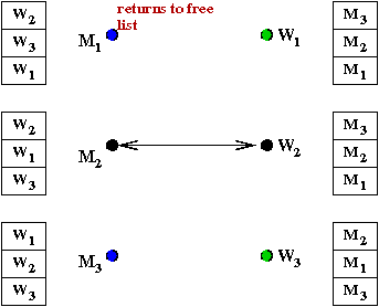
- M1 is back on the free list.
- M3 proposes to W1
→
She accepts
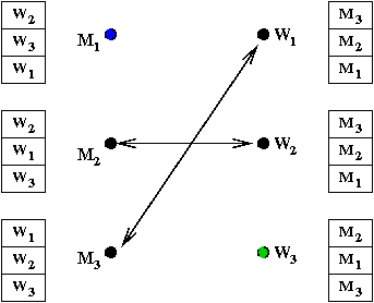
- M1 proposes to W3
→
She accepts
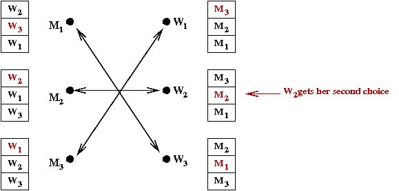
- Done.
Exercise:
Who gets the better deal - men or women?
- In pseudocode:
Algorithm: proposal (M, W)
Input: n men M1,...,Mn and n women W1,...,Wn with their rankings
1.    Add all men to freeList
2.    while freeList is not empty
3.        M = remove a man from freeList
4.        W = highest-ranked woman he has not yet proposed to
5.        if W is unengaged
6.            M and W are engaged
7.        else if W prefers M to her fiance M'
8.            M and W are engaged
9.            M' is placed on the free list
10.       endif
11.   endwhile
Does the algorithm work?
- Does it end?
- A is only rejected once by a woman.
- This can happen only a finite number of times.
- Is the marriage stable?
- Suppose man M and woman W each prefer
the other to their current spouses.
- Suppose M is married to A and
W is married to B.
- M proposed to W before A.
- Case 1: A rejected M's proposal.
→
She was already engaged to someone better than M.
→
But then, she couldn't be married to someone lower than M.
→
Contradiction!
- Case 2: A dumped M.
→
She must have found someone better.
→
Contradiction!
- Running time: O(n2)
- At each step, an engagement occurs.
- Each woman can only be engaged to n men.
→
Only O(n2) engagements possible.
- A marriage is male-optimal if:
- The marriage is stable.
- Among all stable marriages, each male gets his top choice (among the choices in the stable marriages).
- Similar definition for male-pessimal, female-optimal, and female-pessimal.
- Result: the proposal algorithm results in a marriage that
is male-optimal and female-pessimal.
History of the stable marriage problem:
- Has its origins in hospital-resident matching:
- 1900-1945: No regulation
→
No information, chaotic assignments
- 1945-51: tight deadline
→
Bad for residents and second-choices (market unraveling)
- 1952: Mullin-Stalnaker algorithm
→
Turned out to be unstable.
- This was re-designed into the Boston-Pool algorithm that
produced stable assignments.
→
Became the algorithm of choice for the National Resident
Matching Program (NRMP).
- 1984: Boston-Pool shown to be hospital-optimal.
- 1998: Roth-Peranson algorithm used in NRMP
- Handles couples.
- Incomplete rank lists.
- Limited seats for certain specialties.
- 2004: Anti-trust lawsuit prompted enaction of a law
to asserting its pro-competitiveness.
Other applications and developments:
- All kinds of medical specialities.
- New York and Boston schools.
- Variations: stable-roomate problem, college admissions, blacklists.
- Other studies: how to handle cheating.
- If, with different numbers of men and women, a
stable marriage is not possible, it is NP-hard to find
the largest possible stable marriage.
- Real marriages: see scientificmatch.com.
Graph Matching
A natural extension to the marriage problem is the matching problem:
- A graph G=(V,E) is bipartite if the vertices V
can be partitioned into two sets V = X U Y such that
there is no edge between an X vertex and a Y vertex.
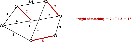
- Example of a weighted bipartite graph:
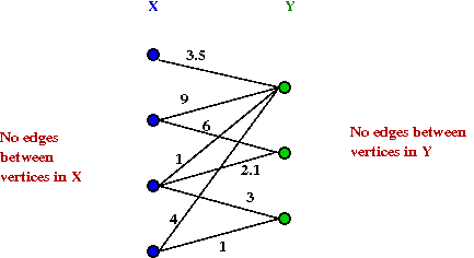
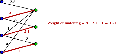
- A matching is a subset of edges such that no two
edges share an endpoint.
- Example of a matching:
- Relationship to marriage problem:
- Think of X as representing males, Y as females.
- An edge weight is the "value" of a pairing.
- Goal: find the maximum weight matching.
- A further generalization: when G is non-bipartite, e.g.
Types of matching problems:
- Unweighted bipartite matching
- O(VE) augmenting path algorithm.
- Improved to O(E√V) in 1973 by Hopcroft and Karp.
- Weighted bipartite matching
- O(V2E) so-called Hungarian algorithm.
- Devised by Harold Kuhn in 1955.
- Kuhn called it the Hungarian method because it was
based on a few ideas by Hungarian mathematicians D.Konig
and E.Egervary.
- Can be improved to O(V2log(V) + VE) using a
Fibonacci heap.
- Unweighted general (non-bipartite) graph matching
- Celebrated "blossoms" algrorithm by Jack Edmonds in 1965.
- O(V2E) complexity.
- Recall: Edmonds introduced the idea of polynomial
vs. exponential algorithms.
- Weighted general (non-bipartite) graph matching
- Blossoms algorithm can be modified to work for weighted version.
- Improvements by Gabow and collaborators to
O(EVlog(V)) in 1986 and 1989.
- An LP formulation can be solved with a polynomial number
of constraints in O(V4) time.
Text matching (mining)
There are many versions of this problem, but let's start
with the most elementary version:
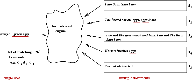
- We have a (large) collection of documents.
- Each document is a "bag of words".
- A user query is also a "bag of words".
- The objective: return the most relevant documents to the user.
- Note: this is a version of the marketplace problem
- The user intention is "less clear".
- But sellers (documents) have no resource limitations.
- Here, words are the most basic unit:
- However, one often uses word stems
→
e.g., "hatch" instead of "hatches" or "hatching".
- Sometimes synonyms are used, but this has been found
to have limited use.
- There are variations of the basic problem that we won't consider:
- Iterated query refinement, and question-answer frameworks.
- Topic detection and classification.
- Cross-language languages retrieval.
- Each year the the TREC
conference puts out challenge problems in various categories.
Three different approaches to text retrieval:
- Boolean queries:
- User specifies a query using Boolean operators such as:
("green" AND "eggs" AND "ham") OR ("Horton")
- System finds all documents that exactly match the query.
- Note: documents are not ranked
→
Either a document matches the query or not.
- User studies show that only a few "power users" find
this approach useful.
- Relevant-ranked queries are the most preferred form of search.
- Probabilistic-relevance approach:
- Identify relevant documents.
- For each relevant document, compute
Pr[document is relevant].
- Rank in order of probabilistic-relevance.
- Vector-space model:
- Treat each document as a vector in document-space.
- A query is also a vector in the same space.
- Find close matches and list in order of "closeness".
Let's look into the details of the latter two:
Data mining
What is data mining?
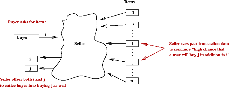
- Example: Grocery store
- Suppose a grocer examines past transaction data to conclude
"When a customer buys wine (item i) they also buy
specialty cheese (item j) with high probability"
- Then, by placing cheese near the wine shelf, a grocer
increases the chance of an impulse purchase.
- Such associations can be extracted from
transaction data.
- Example: banking
- Suppose a bank discovered that
"77% of loan defaults involved a car loan to someone aged
18-21 for a red sportscar"
- Then, such an inference from the data can drive policy.
- Online shopping:
- Amazon and others present "recommended items".
- These are based on other customers' purchases.
- This extraction of patterns from standard database data is
called data mining.
- History:
- Late 1980's: rule extraction or knowledge discovery in databases.
- An early landmark paper in 1993
[Agra1993]
defined the association-rule problem which
spurred the development of the field.
- The association-rule problem:
- The input: a database table of transaction data such as:
         Transaction #1:  eggs, milk, cookies
         Transaction #2:  beer, chips, pretzels, popcorn
         ...
         Transaction #i:  beer, chips, diapers
         ...
         Transaction #6,391,202: wine, brie, diapers
- Goal: identify rules of the sort:
"60% of the time diapers are purchased, beer and chips
are also purchased".
- The challenge: extract such rules efficiently from very
large databases.
- For more details:
see these notes on data mining.
Amazon's recommendation engine:
- For every pair of items, Amazon identifies a "co-purchase" score.
- Algorithm:
1.   Initialize purchase-pair-set S = φ
2.   for each item i
3.       for each customer c who purchased i
4.           for each item j purchased by c
5.               S = S U {(i,j)}
6.           endfor
7.       endfor
8.   endfor

9.   for each item-pair in φ
10.         compute similarity-score for (x,y)
            // The score is the cosine distance between two items.
11.      endfor
12.  endfor
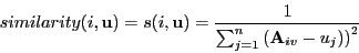
- What is the similarity-score?
- One simple way: the number of customers that bought both.
→
To compute this, add a counter after line 5 above.
- Another way: compute the "cosine" distance treating items
as column vectors in the matrix A where
Aij = 1 if user i bought
item j.
- Note: Amazon's algorithm does not find similar users
to make recommendations.
Collaborative filtering
What is collaborative filtering (CF)?
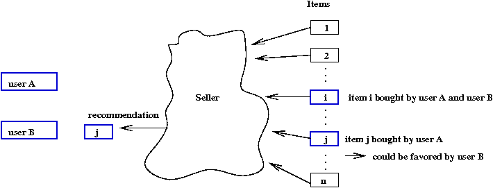
- From a user's point of view:
→
"I'd like to know what users like me rate highly"
- From a seller's point of view:
→
I'd like to predict what a user would like based on
ratings or purchases from similar users.
- Origin of the term:
- Email system add-on called Tapestry devised by Goldberg et al
[Gold1992] in 1992.
- Users rate email content or record actions "e.g., replied".
- Users filter email based on others' ratings or actions
→
e.g., "Include all emails that Alice replied to".
- The current use is more technical:
- Users rate some items.
- Goal: predict a user's rating of some item they have not rated.
- This approach was developed by the pioneering
GroupLens project on movie ratings in 1994
[Resn1994].
- Define ratings matrix Aij as follows
Aij = user i's rating of item
j.
- Example with 5 users, 8 items:
- The Netflix Challenge:
- Started in October 2006.
- Ratings from 480,189 users on 17,770 movies.
- Total of 100,480,507 ratings.
- Test test of about 1 million missing ratings.
- Goal: predict missing ratings.
- Challenge: beat Netflix's own algorithm by 10%.
- Won by a combination of teams in 2009.
Approaches to CF:
- Data-driven approach:
- Use the data to compute similarities between users or items.
- Generate a prediction based on the data from similar users/items.
- Also called the memory-based approach.
- Model-driven approach:
- Use the data to build a statistical model.
→
And estimate that model's parameters.
- Use model for prediction.
- Hybrid approaches: these combine the above two.
- Henceforth, we'll assume the following version of the
CF problem:
- We are given the user-item ratings matrix A.
- The goal: predict missing entry Auv.
→
User u's rating of item v.
The data-driven approach:
- This approach was pioneered by the GroupLens project
[Resn1994].
- Since then it has been refined and modified by several others.
- Two kinds:
- User-similarity: find similar users to user
u who have rated v and use their ratings.
- Item-similarity: find similar items to item v,
and use the ratings of these items.
- Let's first focus on the user-similarity approach.
Algorithm: userSimilarity (A, u, v)
Input: ratings matrix A, and desired missing entry A[u,v]
// Compute distances to other users.
1. for each user i
2. s[i] = similarity (i, u)
3. endfor
// Find a set of "close" or similar users.
4. similar-user-set S = φ
5. for each user i that has rated item j
6. if similarEnough (i, u)
7. add i to S
8. endif
9. endfor
// Use the ratings of these users to predict user u's rating v.
10. r = combineRatings (S, v)
11. return r
- The details of
similarity()
similarEnough()
and
combineRatings()
differentiate various algorithms in this category.
→
We will only look at a few ideas - see the references for
more details.
- First, observe that rows of A are
user-vectors:
Exercise:
What is the cosine of the angle between the "Alice" and "Dave" vectors?
What is the cosine of the angle between the "Alice" and "Chen" vectors?
- Similarly, columns are item-vectors:
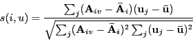
- Computing similarity: several ways
- Inverse Mean-square difference between the vectors for two rows.
- Cosine of angle between vectors.
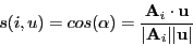
- Pearson-correlation between the vectors.
- Many ways of identifying the "close-enough" ones:
- Keep the K closest ones (where K is an
algorithm parameter).
- Maintain a threshold δ and keep those users
within this distance.
- Combining ratings from close users on item v:
- Average their ratings.
- Take a weighted average, weighted by similarity
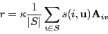
- Offset weighted average by the mean.
→
Because some users tend to have high averages or low averages.
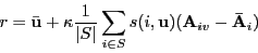
- Note: κ is a normalizing factor.
- More complex statistical techniques such as multiple-regression
have been tried
[Hill1995].
- The item-similarity approach:
[Sarw2001]
- Recall: our goal is to estimate Auv.
- In this approach: find a set of similar items I.
- Use the ratings of users for the items in I.
- How to find similar items?
- Use the same types of vector-similarity measures as in
comparing users.
→
Only this time, we use the columns of A.
- Thus, items are similar if many users tend to rate them similarly.
- How to combine ratings?
- Again, using the same ideas as in user-similarity.
- Find those items in I that have ratings for
user u.
- Combine those ratings as above.
Model-based approaches:
- Model-based approaches try to uncover some underlying
"structure" if such a structure exists or can be approximated.
- For example: we "know" intuitively that users can
be divided into "sci-fi movies", "romance movies" and the like.
- If we can identify the user as one of these types,
our prediction success might go up.
- We'll next look at a few model-based approaches.
Simple clustering:
- Create user categories.
→
These could be done by hand (e.g., "sci-fi", "romance" etc).
- For each user, identify their category.
- To compute Auv:
- Identify u's category c.
- Find users in c who have rated v.
- Combine their ratings using some kind of averaging.
- How do we classify users into categories?
- Create "fake" user vectors, one for each category.
→
These serve as prototypes for the categories (ideal users).
- Each such vector will have high ratings for the movies
in that category, low for the others.
→
This means we need to "know" these categories.
- Then, one can use vector-similarity with these category
prototypes.
- Example:
                  1   2   3   4   5   6   7   8
         Alice  |     1       5   5       3     |
         Bob    | 4       2           1       2 |
         Chen   |     1                         |
         Dave   |     2       4           3     |
         Ella   |     5       1   1           5 |
Sci-fi | 0 5 0 5 0 0 0 0 | // Movies 3 and 5 are sci-fi movies. Rest of the ratings are 0.
- How to do this without pre-defined categories:
- Initially, we'll create K empty clusters.
- Initially, assign each user to a random cluster.
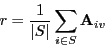
- Treat each user-vector as a point in n space.
- Compute the average "point" (the cluster mean) in each cluster.
- Now, for each user, identify closest mean and re-classify
the user accordingly.
- Repeat.
This is called K-means clustering.
Algorithm: K-means (A, u, v)
Input: ratings matrix A, and desired missing entry A[u,v]
1.   for each user i
        // Initially assign each user to a random cluster.
2.      cluster[i] = random (1, K)
3.   endfor

4.   while not converged
        // Find the mean of each cluster and assign users to the cluster whose mean they are closest to.
5.      Mk = computeMean (Ck)
6.      for each user i
7.         find closest cluster mean k
8.         cluster[i] = k
9.      endfor
10.  endwhile

11.  k = cluster for user u
12.  S = users in Ck that have rated v
13.  r = combineRatings (S, v)
14.  return r
A probabilistic approach: the Naive-Bayes method
- Let user u's vector of ratings be
(u1,...,un).
- We want to predict uv, one of the missing ones.
- Suppose we treat this as the random variable Uv.
- Then, in a 5-point rating system, such a random variable
can take values 1,2, ... ,or 5.
- We ask the question: what is
Pr[Uv=r | u1,...,un].
- That is, given the known ratings
(u1,...,un).
what is the probability that the unknown one is r?
(Where r is either 1,2, ..., or 5.)
- If we had these probabilities, how do we actually pick the rating?
→
The simplest way: pick the rating r whose
probability
Pr[Uv=r | u1,...,un].
is highest.
- One way to do this:
- Find other users who have rated both
(u1,...,un).
and uv.
- Estimate
Pr[Uv=r | u1,...,un].
from this data by simple averaging.
- For this to be possible, the matrix A needs to be
dense
→
The data has to be rich enough to find many such "high-overlap" users.
- Unfortunately, this is not the case in practice (at least for movie data).
- Some applications explicitly ask the user to rate 10-15 items
so that all users have rated the same items.
- So, let's examine a way around this problem: the Naive Bayes approach.
- Using Bayes' rule
Pr[Uv=r | u1,...,un]
= Pr[u1,...,un | Uv=r]
Pr[Uv=r] / Pr[u1,...,un]
- Note that Pr[u1,...,un] is the
simply the user-independent probability of observing
the known ratings.
- This is a "constant" for the system.
→
We will absorb it in a normalizing constant.
- Thus,
Pr[Uv=r | u1,...,un]
∝
Pr[u1,...,un | Uv=r]
Pr[Uv=r]
- Next, we will assume independence between items and write
Pr[u1,...,un | Uv=r]
=
Πi
Pr[ui | Uv=r]
- Each of these can be estimated because there's hope that
we can find users who've rated both item v and
item i.
- Similarly, Pr[Uv=r] can be estimated
from the column vector for item v.
- Thus, we can estimate
Pr[Uv=r | u1,...,un]
=
κ
Pr[u1,...,un | Uv=r] Pr[Uv=r]
=
κ
Pr[Uv=r]
Πi
Pr[ui | Uv=r]
where κ is a normalizing constant.
- In fact, we don't need to worry about the normalizing
constant at all:
- We are interested in picking that rating r
for which
Pr[Uv=r | u1,...,un]
is largest.
- This is the same as picking the rating for which
Pr[Uv=r]
Πi
Pr[ui | Uv=r]
is highest (without the normalizing constant).
- Let's outline this approach with some pseudocode:
Algorithm: naiveBayes (A, u, v)
Input: ratings matrix A, and desired missing entry A[u,v]
      // Estimate Pr[Uv=r].
1.    for each rating value r
2.        num_v_r = # users that rated v as r
3.        num_v = # users that rated v
4.        RatingEstimate[r] = num_v_r / num_v
5.    endfor

      // Estimate Pr[ui | Uv=r] for each possible i and r.
6.    for each r
7.        for each item j ≠ v
8.            num_u_j_r = # users that rate j as uj and v as r
9.            num_v_r = # users that rated v as r
10.           conditionalRating[j] = num_u_j_r / num_v_r
11.       endfor
12.   endfor

      // Estimate Pr[Uv=r |  u1,...,un] using the product and identify the largest.
13.   rmax = 0
14.   for each r
15.       product[r] = ratingEstimate[r]
16.       for each item j ≠ v
17.           product[r] = product[r] * conditionalRating[j]
18.       endfor
19.       if product[r] > rmax
20.           rmax = product[r]
21.       endif
22.   endfor

23.   return rmax
- The Bayes approach has been used in book recommendation
engines
[Moon1999].
Machine learning:
References and further reading
[WP-1]
Wikipedia entry on Collaborative filtering.
[WP-2]
Wikipedia entry on the Stable Marriage problem.
[Agra1993]
R.Agrawal, T.Imielinski and A.Swami.
Mining Association Rules between Sets of Items in Large Databases.
SIGMOD, 1993.
[Agra1994]
R.Agrawal and R.Srikant.
Fast algorithms for mining associative rules.
VLDB, 1994.
[Basu1998]
C.Basu, H.Hirsh and W.Cohen.
Recommendation as classification: using social and content-based information
in recommendation.
AAAI ˇ¦98, pp. 714ˇV720, July 1998.
[Bill1998]
D.Billsus and M.Pazzani.
Learning collaborative information filters.
Int. Conf. on Machine Learning (ICML ˇ¦98), 1998.
[Bree1998]
J.Breese, D.Heckerman and C.Kadie.
Empirical analysis of predictive algorithms for collaborative filtering.
Proc. 14th Conf. Uncertainty in Artificial
Intelligence (UAI ˇ¦98), 1998.
[Deer1990]
S.Deerwester, S.T.Dumais, G.W.Furnas, T.K.Landauer and R.Harshman.
Indexing by latent semantic analysis.
J.Am.Soc.Info.Sci., vol.41, no. 6, pp.391-407, 1990.
[Gale1962]
D.Gale and L.S.Shapley.
College Admissions and the Stability of Marriage.
American Mathematical Monthly, Vol.69, pp.9-14, 1962.
[Gold1992]
D.Goldberg, D.Nichols, B.M.Oki and D.Terry.
Using collaborative filtering to weave an information Tapestry.
Comm. ACM, vol. 35, no. 12, pp. 61ˇV70, 1992.
[Grif2000]
J.Griffith and C.O'Riordan.
Collaborative filtering.
Technical report NUIG-IT-160900, National University of Ireland.
[Herl1999]
J.L.Herlocker, J.A.Konstan, A.Borchers and J.Riedl.
An algorithmic framework for performing collaborative
filtering.
Conf. Res. Dev. Information Retrieval (SIGIR ˇ¦99),
pp.230ˇV237, 1999.
[Hill1995]
W.Hill, L.Stead, M.Rosenstein and G.Furnas.
Recommending and evaluating choices in a virtual
community of use.
ACM Conf. Human Factors in Computing, pp.194-201, 1995.
[Kore2009]
Y. Koren,
The BellKor Solution to the Netflix Grand Prize.
(2009).
[Lind2003]
G.Linden, B.Smith and J.York.
Amazon.com recommendations: item-to-item collaborative
filtering.
IEEE Internet Computing, January 2003.
[Mann2008]
C.D.Manning, P.Raghavan and H.Schutze.
Introduction to Information Retrieval,
Cambridge University Press. 2008.
(Also available in
PDF.)
[Moon1999]
R.J.Mooney and L.Roy.
Content-Based Book Recommending Using Learning for Text Categorization.
ACM Conf. Digital Libraries, 1999.
[Piot2009]
M.Piotte and M.Chabbert.
The Pragmatic Theory solution to the Netflix Grand Prize,
2009.
[Resn1994]
P. Resnick, N. Iacovou, M. Suchak, P. Bergstrom, and J. Riedl.
Grouplens: an open architecture for collaborative filtering of netnews.
Proc. ACM Conf. Computer Supported Cooperative Work,
pp. 175ˇV186, New York, NY, 1994.
[Roth2008]
A.E.Roth
Deferred Acceptance Algorithms: History, Theory, Practice,
and Open Questions.
Int. J. Game Theory,
Vol. 36, March, 2008, pp.537-569.
[Sarw2001]
B.M.Sarwar, G.Karypis, J.A.Konstan and J.Riedl.
Item-based collaborative filtering recommendation algorithms.
10th Int. Conf. World Wide Web (WWW ˇ¦01),
pp. 285ˇV295, May 2001.
[Sing2001]
A.Singhal.
Modern information retrieval: An overview.
Bulletin of the IEEE Computer Society Technical
Committee on Data Engineering, 24:4, 2001.
[Su2009]
X.Su and T.M.Khoshgoftar.
A survey of collaborative filtering techniques.
Adv. AI, Vol. 2009,
Article ID 421425, 19 pages, 2009. doi:10.1155/2009/421425.
[Tosc2009]
A. Toscher, M. Jahrer, R. Bell.
The BigChaos Solution to the Netflix Grand Prize.
2009.
[Unga1998]
L.H.Ungar and D.P.Foster.
Clustering methods for collaborative filtering.
Workshop on Recommendation Systems, 1998.