The Minimum Spanning Tree (MST) problem is a classic
computer science problem.
We will study the development of algorithmic ideas for this
problem, culminating with
Chazelle's O(m α(m,n))-time algorithm,
an algorithm that easily meets the "extreme" criterion.
A preview:
- How is the MST problem defined?
- Simple algorithms: Kruskal and Jarnik-Prim.
- A generalization from the past: Boruvka.
- The basic binary heap and its descendants.
- A randomized algorithm.
- Chazelle's and Pettie's (independently discovered) algorithms.
Our presentation will pull together material from various sources - see the
references below. But most of it will come from
[Eisn1997],
[Pett1999],
[CS153],
[Weis2007].
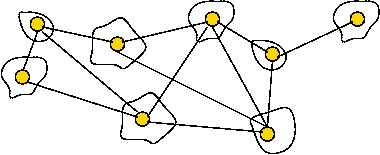
Background: what is a graph?
Informal definition:
- A graph is a mathematical abstraction used to represent
"connectivity information".
- A graph consists of vertices and edges that
connect them, e.g.,
- It shouldn't be confused with the "bar-chart" or "curve" type
of graph.
Formally:
- A graph G = (V, E) is:
- a set of vertices V
- and a set of edges E = { (u, v): u and v are vertices }.
- Two types of graphs:
- Undirected graphs: the edges have no direction.
- Directed graphs: the edges have direction.
- Example: undirected graph
- Edges have no direction.
- If an edge connects vertices 1 and 2, either
convention can be used:
- No duplication: only one of (1, 2) or (2, 1)
is allowed in E.
- Full duplication: both (1, 2) and (2, 1)
should be in E.
- Example: directed graph
- Edges have direction (shown by arrows).
- The edge (3, 6) is not the same as the edge (6,
3) (both exist above).
- For the MST problem: we will only use undirected graphs.
Depicting a graph:
- The picture with circles (vertices) and lines (edges) is
only a depiction
→ a graph is purely a mathematical abstraction.
- Vertex labels:
- Can use letters, numbers or anything else.
- Convention: use integers starting from 0.
→ useful in programming, e.g. degree[i] = degree
of vertex i.
- Edges can be drawn "straight" or "curved".
- The geometry of drawing has no particular meaning:
Graph conventions:
- What's allowed (but unusual) in graphs:
- Self-loops (occasionally used).
- Multiple edges between a pair of vertices (rare).
- Disconnected pieces (frequent in some applications).
Example:
- What's not (conventionally) allowed:
- Mixing undirected and directed edges.
- Re-using labels in vertices.
- Bidirectional arrows.
Exercise:
If we disallow multiple edges and self-loops, what is the maximum
number of edges in an undirected graph with n vertices?
What is this number in order-notation?
Definitions (for undirected graphs):
- Degree of a vertex: number of edges incident to it.
Neighbors:
Two vertices are neighbors (or are adjacent) if
there's an edge between them.
Paths:
- Path: a sequence of vertices in which successive
vertices are adjacent.
- A simple path does not repeat any vertices (and
therefore edges) in the sequence.
- A cycle is a simple path with the same vertex as the
first and last vertex in the sequence.
Connectivity:
two vertices are connected if there is a
path that includes them.
Weighted graph:
- Sometimes, we include a "weight" (number) with each edge.
- Weight can signify length (for a geometric application)
or "importance".
- Example:
Euclidean graph:
- The vertices are points in the plane.
- Edges are implied (all pairs) with Euclidean distance as weights.
- Note: one can define a version for d-dimensions.
Trees:
- A tree is a connected graph with no cycles.
- A spanning tree of a graph is a connected subgraph
that is a tree.
Data structures for graphs:
- Adjacency matrix.
- Key idea: use a 2D matrix.
- Row i has "neighbor" information about vertex i.
- Here, adjMatrix[i][j] = 1 if and only if there's an edge
between vertices i and j.
adjMatrix[i][j] = 0 otherwise.
- Example:
      0 1 1 0 0 0 0 0
      1 0 1 0 0 0 0 0
      1 1 0 1 0 1 0 0
      0 0 1 0 1 0 1 0
      0 0 0 1 0 0 1 0
      0 0 1 0 0 0 1 1
      0 0 0 1 1 1 0 0
      0 0 0 0 0 1 0 0
Note: adjMatrix[i][j] == adjMatrix[j][i] (convention for
undirected graphs).
- Adjacency list.
- Key idea: use an array of vertex-lists.
- Each vertex list is a list of neighbors.
- Example:
- Convention: in each list, keep vertices in order of insertion
→ add to rear of list
- Both representations allow complete construction of the graph.
- Advantages of matrix:
- Simple to program.
- Some matrix operations (multiplication) are useful in some
applications (connectivity).
- Efficient for dense (lots of edges) graphs.
- Advantages of adjacency list:
- Less storage for sparse (few edges) graphs.
- Easy to store additional information in the data structure.
(e.g., vertex degree, edge weight)
- Implementations for MST use adjacency lists.
Defining the MST problem
With this background, it's going to be easy to state the MST problem:
find the spanning tree of minimum weight (among spanning trees):
- Input: a weighted, connected graph.
- Output: find a sub-graph such that
- The sub-graph is a connected tree.
- The tree contains all graph vertices.
→ it's a spanning tree.
- The tree weight is defined as the sum of edge-weights in
the tree.
- The tree weight is the least among such spanning trees.
Exercise:
- "Eyeball" the weighted graph below
and find the minimum spanning tree, and the shortest path from vertex 0
to vertex 6.
- Try the example given to you in class.
Some assumptions and notation for the remainder:
- Let n = |V| = number of vertices.
- Let m = |E| = number of edges.
- We will assume unique edge weights. If this is not true,
some arbitrary tie-breaking rule can be applied.
→
It simplifies analysis.
Minimum Spanning Trees: Two Key Observations
The Cut-Edge Observation:
- Consider a partition of the vertices into two sets.
- Suppose we re-draw the graph to highlight edges going from
one set to the other: (without changing the graph itself)
- Cut-edge: an edge between the two sets.
- Consider the minimum-weight edge between the sets.
(Assume the edge is unique, for now).
- The minimum-weight edge must be in the minimum spanning tree.
Exercise:
Why?
Prim's algorithm (a preview):
- Start with Set1 = {vertex 0}, Set2 = {all others}.
- At each step, find an edge (cut-edge) of minimum-weight
between the two sets.
- Add this edge to MST and move endpoint from Set2 into Set1 .
- Repeat until Set1 = {all vertices}.
The Cycle Property:
- First, note: adding an edge whose end-points are in the MST will
always cause a cycle.
- Consider adding an edge that causes a cycle in current MST.
- Suppose the edge has weight larger than all edges in cycle
→ no need to consider adding edge to MST.
- Therefore, if edges are added in order of (increasing)
weight
→ no need to consider edges that cause a cycle.
Kruskal's algorithm (a preview):
- Sort edges in order of increasing weight.
- Process edges in sort-order.
- For each edge, add it to the MST if it does not cause a cycle.
Kruskal's Algorithm
Key ideas:
- Sort edges by (increasing) weight.
- Initially, each vertex is a solitary sub-graph (MST-component).
- Start with small MST-component's and grow them into one large MST.
- Need to track: which vertex is in which component (i.e., set).
Exercise:
Show the steps in Kruskal's algorithm for this example:
Implementation:
- High-level pseudocode:
Algorithm: Kruskal-MST (G)
Input: Graph G=(V,E) with edge-weights.

1.   Initialize MST to be empty;
2.   Place each vertex in its own set;
3.   Sort edges of G in increasing-order;
4.   for each edge e = (u,v) in order
5.       if u and v are not in the same set
6.           Add e to MST;
7.           Compute the union of the two sets;
8.       endif
9.   endfor
10.  return MST

Output: A minimum spanning tree for the graph G.
- Now, let's use a union-find algorithm and explain in more
detail:
Algorithm: Kruskal-MST (adjMatrix)
Input: Adjacency matrix: adjMatrix[i][j] = weight of edge (i,j) (if nonzero)

1.   Initialize MST to be empty;

     // Initialize union-find algorithm and
     // place each vertex in its own set.
2.   for i=0 to numVertices-1
3.       makeSingleElementSet (i)
4.   endfor

5.   sortedEdgeList = sort edges in increasing-order;

6.   Initialize treeMatrix to store MST;

     // Process edges in order.
7.   while sortedEdgeList.notEmpty()
8.       edge (i,j) = extract edge from sortedEdgeList.
         // If edge does not cause a cycle, add it.
9.       if find(i) != find(j)
10.          union (i, j)
11.          treeMatrix[i][j] = treeMatrix[j][i] = adjMatrix[i][j]
12.      endif
13.  endwhile

14.  return treeMatrix

Output: adjacency matrix represention of tree.
Analysis: (adjacency list)
- To place edges in list: simply scan each vertex list once.
→ O(m) time.
- Sorting: O(m log(m)).
- O(log(n)) per union or find.
- Total: O(m)+ O(m log(m)) + O(m log(n))
→ O(m log(m))
→ O(m log(n))
Prim's Algorithm
Key ideas:
- Start with vertex 0 and set current MST to vertex 0.
- At each step, find lowest-weight edge from an MST vertex to a non-MST
vertex and add it to MST.
- To record the weight of each edge, we will associate edge weight
with the vertex that's outside the MST.
- We will associate a "priority" with each vertex:
- Priority(v) is defined only for v not in current MST.
- Intuitively, priority(v) = cost of getting from current MST to v.
- For example, consider node A with priority(A) = 3.1
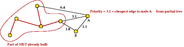
- priority(A) changes to 1.1 after B is added.
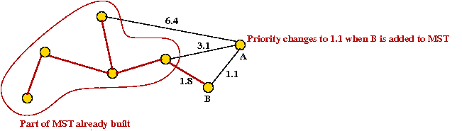
Example:
Implementation:
- High-level pseudocode:
Algorithm: Prim-MST (G)
Input: Graph G=(V,E) with edge-weights.

1.   Initialize MST to vertex 0.
2.   priority[0] = 0
3.   For all other vertices, set priority[i] = infinity
4.   Initialize prioritySet to all vertices;
5.   while prioritySet.notEmpty()
6.       v = remove minimal-priority vertex from prioritySet;
7.       for each neighbor u of v
9.           w = weight of edge (v, u)
8.           if w < priority[u]
9.               priority[u] = w        // Decrease the priority.
10.          endif
11.      endfor
12.  endwhile

Output: A minimum spanning tree of the graph G.
Exercise:
Consider line 6 in the algorithm above. How long does it
take to execute?
Analysis:
- Each edge is added once to the priority set.
- There are O(n) removals.
- Since each edge is processed once, there are at most
O(m) priority adjustments.
- Thus, if a removal takes time r(n) and
and a priority-decrease takes time d(n)
→
O(n r(n) + m d(n)) time overall.
Exercise:
What is the running time when using a list for the priority set?
- A sorted list.
- An unsorted list.
Enter the data structures, part I: the binary heap
What is a priority queue?
- Keys or key-value pairs are stored in a data structure.
- The operations usually supported are:
- Insert: insert a new key-value pair.
- Delete: delete a key-value pair.
- Search: given a key, find the corresponding value.
- Find minimum, maximum among the keys.
A priority queue with the decreaseKey operation:
- For convenience, we will combine minimum and remove
(delete) into a single operation: extractMin
- We would like to change a key while it's in the data
structure
→ location in data structure also needs to be changed.
- Sorted linked list:
- Potentially O(n) time for decreaseKey
- O(1) time for extractMin
- Unsorted array:
- Potentially O(n) time for extractMin
- O(1) time for decreaseKey
- Can we do better?
- O(log(n)) time for extractMin?
- O(log(n)) time for decreaseKey?
Implementing a priority queue with a binary heap:
- Recall extractMin operation (Module 2):
- Height of heap is O(log(n)) always.
- Each extractMin results in changes along one tree path.
→ O(log(n)) worst-case.
- Implementing decreaseKey:
- Simply decrease the value and swap it up towards root to
correct location.
→ O(log(n)) worst-case.
Using a priority queue with Prim's algorithm:
Algorithm: Prim-MST (adjList)
Input: Adjacency list: adjList[i] has list of edges for vertex i

     // Initialize vertex priorities and place in priority queue.
1.   priority[i] = infinity
2.   priorityQueue = all vertices (and their priorities)
     // Set the priority of vertex 0 to 0.
3.   decreaseKey (0, 0)

4.   while priorityQueue.notEmpty()
         // Extract best vertex.
5.       v = priorityQueue.extractMin()
         // Explore edges going out from v.
6.       for each edge e=(v, u) in adjList[v]
7.           w = weight of edge e;
             // If there's an edge and it's not a self-loop.
8.           if priority[u] > w
                 // New priority.
9.               priorityQueue.decreaseKey (u, w)
10.              predecessor[u] = v
11.          endif
12.      endfor
13.  endwhile

     // ... build tree in adjacency list form ... (not shown)

Output: Adjacency list representation of MST
Analysis:
- Recall: running time of Prim's algorithm depends on
n extract-min's and m decrease-key's.
→
O(n log(n) + m log(n))
= O(m log(n))
Boruvka's algorithm
It turns out that neither Prim nor Kruskal were the first
to address the MST problem
[Grah1985]:
- First, note: Kruskal's algorithm was published in 1956, Prim's in 1957.
- A solution to the problem was first published
in 1926 by Czech mathematician Otakar Boruvka (1899-1995)
[WP-2].
- The problem is itself thought to have been first addressed
in 1938 by G.Choquet.
- The essence of Prim's algorithm first appeared in a
1930 paper by V.Jarnik written in Czech.
- Dijkstra re-discovered the algorithm in 1959.
→
Some books now call this the Jarnik-Prim-Dijkstra algorithm.
- Kruskal and Prim both worked at AT&T Bell Labs,
though neither knew of each other until later.
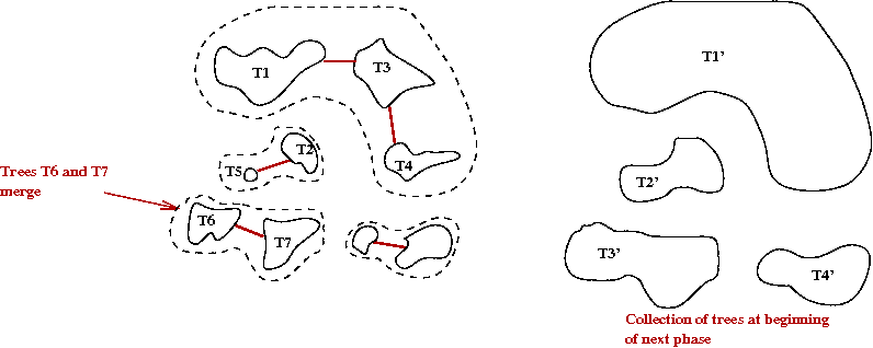
Key ideas in Boruvka's algorithm:
- Start with each vertex as its own tree.
- At each Boruvka phase:
- Identify the cheapest edge leaving each tree.
- Merge the trees joined by these edges.
- Why does this work?
- The cheapest edge going out from a tree T is the
cheapest edge between T and "the outside world"
→
By the cut-edge property, it must be in the MST.
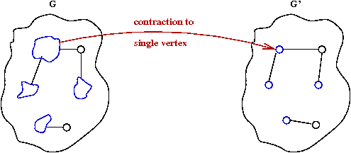
Boruvka's algorithm with edge contractions:
- What is an edge contraction?
- Merge the two nodes on either side into one new node.
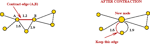
- Keep cheapest edge among multiple edges to neighbors.
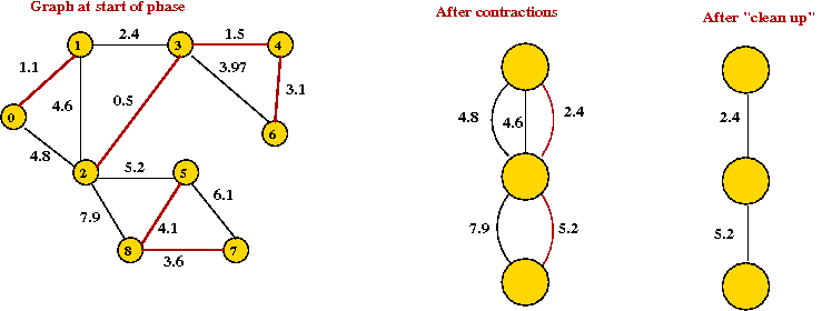
- The algorithm with contractions:
Algorithm: Boruvka (G)
Input: Graph G = (V, E)
1.   Create graph F = (V, φ)     //No edges in F.
2.   while F not connected
3.      for each component in F
4.         add cheapest outgoing edge to MST
5.      endfor
6.      Contract added edges in F and G
7.   endwhile
- Example:
Analyis:
- Let Vi be the vertex set after the
i-th phase.
- Each contraction reduces the vertex set by at least half
→
|Vi+1| ≤ ½ |Vi|.
→
There are at most O(log n) phases.
- In each phase, we examine at most O(m) edges
→
O(m log(n)) time overall.
- This is as good as Prim+BinaryHeap.
Enter the data structures, part II: the fibonacci heap
First, the precursor to the fib-heap: the binomial heap
[Vuil1978].
- The binomial heap is a radical departure from
standard data structures in one way:
→
Instead of one tree, it uses a collection of trees.
- To avoid confusion, we'll call the whole structure a
binomial queue.
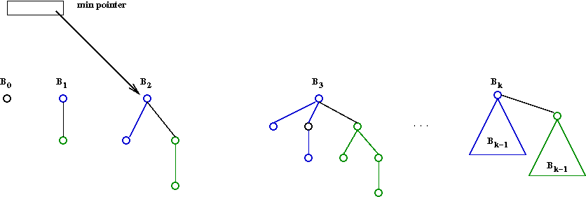
- A binomial queue is:
- A collection of binomial trees.
- Each binomial tree in the queue is min-heap-ordered,
with nodes that can have more than two children,
and has a certain structure (see below).
- Recall that min-heap order means: each parent is "less" than
its children.
- A binomial tree Bk of order k
is a heap-ordered tree defined recursively:
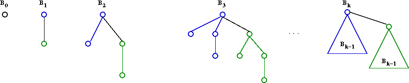
- B0 is a node by itself.
- Bk is the tree you get by taking two
Bk-1 trees and making one a right child
of the other's root.
- A queue can have at most one tree of each order.
→
e.g., at most one B3 tree.
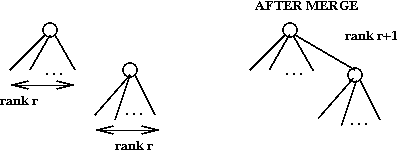
- The tree merge operation:
- Two Bk trees can be joined as above
to make a Bk+1 tree.
- To maintain min-order, the lesser Bk
root becomes the Bk+1 root.
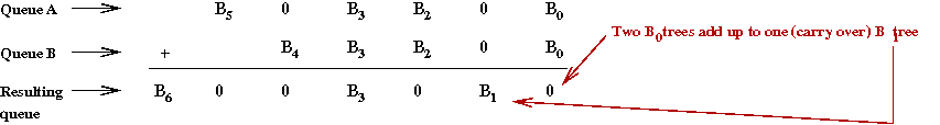
- The queue merge operation:
- Two binomial queues can be merged using something
like binary addition (with carryover).
- Example: suppose we have two queues
- Insert operation:
- Make a new B0 tree and merge that into the
existing queue.
- A min pointer:
- The true minimum can be in any one of the trees.
- Keep an external pointer to the running minimum:
- Extract-min operation:
- First, here's another view of a binomial queue (useful for extract-min):
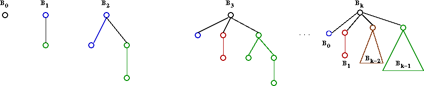
- Remove min node (a root of some Bk).
- This will leave child trees B0,
B1 ... Bk-1.
- Merge each of these into the rest of the queue.
- Decrease-key operation:
- Decrease value and make heap-adjustments within the tree.
→
Same as in binary heap.
Exercise:
Show that the binomial tree Bk has
2k nodes. Then argue that there are
at most O(log n) trees.
Binomial queue analysis:
- At first it seems we have the following:
- Insert: O(log n) because of all the "carry"
operations that might occur.
- Extract-min: O(log n) because all the subtrees
need to be added (a queue-merge operation).
- Decrease-key: O(log n) as in binary heap.
- However, consider this:
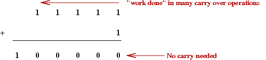
- When a carry ripples, it also leaves behind 0's.
→
Reduces the need for carries in the future.
→
Over time, the actual number of carries may not be high.
- We want to account for the average cost of an operation over time
→
Called amortized analysis.
- This is still a worst-case (not average).
- It's really a "worst possible average cost".
- The idea of a potential function:
- In physics, "work done" results in storing potential energy.
- The analog here: "work done" in carries stores "good" zeroes.
- Amortized analysis of insert-operation:
- Let Pi = potential = number of 0's after
i-th insert.
- Let Pi - Pi-1 = change in potential.
- Let Ci = true cost of i-th insert.
- Then
Ci = 1 + Pi - Pi-1
i.e., cost = cost-of-new-item + ripple-carry
- Hence, over n operations
Σ >Ci = n + Pn - P0
≤ 2n
- Thus, average cost is
(1/n) Σ Ci = O(1).
- Note:
- Above we equated "potential" with "good" zeroes.
- We could just as easily equate "potential" with "bad" ones.
→
Exactly the same analysis but with change-of-sign for potential.
- Unfortunately: for extract-min and decrease-key, the
amortized time is still O(log n).
The Fibonacci heap [Fred1987]: an overview
- The fibonacci heap is a modification of the binomial such that
- Decrease-key takes O(1) amortized.
- Extract min takes O(log n) amortized.
- Again, we switch to calling it a fibonacci queue
because whole thing is a collection of trees.
- The fib-queue is based on two ideas:
- When a decrease-key occurs, don't repair tree.
→
Instead, "cut out" the subtree where the decrease-key occurs.
- Dispense with the strict binomial-tree properties:
- Dispense with: at most one Bk tree.
- Dispense with: recursive structure of each Bk.
More detail:
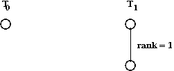
- Define
rank (node) = number of children of the node
rank (tree) = rank (tree's root)
- Maintain a list of trees with min-pointer, as in binomial queue.
- When we merge trees, we will merge two trees of equal rank
and create a one-rank-higher tree.
- Cascading cut:
- When doing a decrease-key, if heap-order is violated,
cut-out node along with subtree:
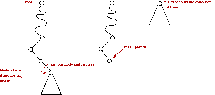
- Then, "mark" the parent.
- A parent with two marks is itself cut-out (as a single-node tree):
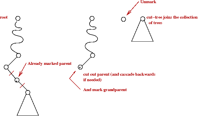
- The cutting cascades upwards as long as marked parents need
to be cut out.
- Lazy-merge:
- When a cut tree is added to main list, simply concatenate
→
Do not perform a merge.
- A merge is performed only during extract-min.
- Decrease-key operation:
- As described above: cut out if needed and cascade backwards.
- Note: O(1) time except for cascades.
→
Will turn out to be O(1) amortized.
- Extract-min operation:
- Remove node as in binomial queue.
- Perform a full merge:
Exercise:
Look up Fibonacci numbers. How are they defined recursively?
Prove the following:
- F0 + ... Fn-2 = Fn - 1.
- Fk = O(φk), where
φ is the golden ratio.
Analysis:
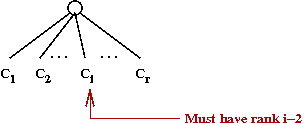
- First, observe:
- If Ci is the i-th youngest child of a
node N, then rank(Ci) ≥ 2
- Proof:
- When Ci is joined with N (during a merge),
N had children C1, C2, ...
Ci-1.
- Nodes are joined only if they have the same rank.
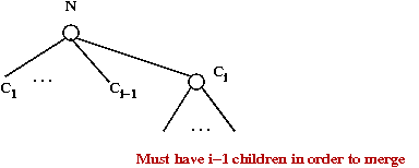
- After merging, it can lose children, but at most one
→
Else, it would itself be cut.
- Thus, it has at least i-2 children.
- Next: a node of rank r has O(Fr)
descendants (not just children).
- Define the "badness" potential as:
potential = #trees + #marked-nodes
- For decrease-key:
- Let C = length of cascade.
- Then, actual cost = C.
- We create O(C) new trees, but reduce marked nodes by O(C).
→
Total change in potential is O(1).
- Amortized cost: O(1).
- For extract-min:
- Does not change # of marked nodes.
- Total # trees is like the total number of 1's in binary addition.
→
Same change in potential over a number of operations.
- Total time is bounded by O(log n), the number of trees.
- Amortized cost: O(log n).
- Note: we have glossed over some details in the analysis. See
the original paper or the description in
[Weis2007].
Back to MST:
- Recall: with Prim's algorithm
- n extract-min's.
- m decrease-key's.
- Thus, for Prim + Fib-heap
→
O(n log(n) + m) bound.
- Compare with:
- Kruskal: O(m log(n))
→
Dominated by O(m log(m)) sort.
- Prim + Binary-heap: O(m log(n))
→
O(n log(n)) extract-min's + O(m log(n)) decrease-key's.
- Boruvka: O(m log(n))
→
From O(log n) phases, each requiring O(m) edge manipulations.
A simple improvement with Boruvka's algorithm:
- Consider the following algorithm:
Perform O(loglog n) phases of Boruvka (with
contractions).
→
This takes O(m loglog(n)) time.
- Apply Prim to the resulting graph.
- Put together all MST edges into single MST.
- Now, we start with n components (the original nodes
as one-node trees).
- After phase 1, there are at most n/2 components.
- After phase 2, at most n/22 components.
- ... after phase k, at most n/2k components.
- Thus, if we do O(loglog n) phases, we'll have
at most n/log(n) components.
→
After contraction, this gives a graph with n/log(n) vertices.
- Applying Prim + Fibonacci on the last graph:
- O(m + n/log(n) log(n)) = O(m + n) time.
- Thus, overall: O(m loglog(n)) time.
→
Fastest so far.
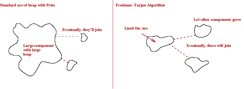
Fredman and Tarjan's Algorithm
Fredman and Tarjan didn't stop with inventing the Fibonacci heap
[Fred1987].
So, is this better?
- The comparison to make is:
- Prim+Fib: O(nlog(n) + m).
- Boruvka+Prim+Fib: O(m loglog(n)).
- Fredman-Tarjan: O(m β(m,n)).
- Obviously, Fredman-Tarjan is better than Boruvka+Prim+Fib.
- What about Prim+Fib?
- Clearly, when m < O(n log n), Fredman-Tarjan is better.
- It is possible [Eisn1997]
to show that for n>16, m β(m,n) = O(nlog(n) + m).
- Thus, overall, Fredman-Tarjan is the best so far.
An improvement to Fredman-Tarjan
Gabow et al (including Tarjan) [Gabow1986]
found a way to improve the Fredman-Tarjan algorithm:
- Recall that Fredman-Tarjan takes O(mβ(m,n)) time.
- Suppose one could reduce the "work" per phase to
O(m/p) for some judiciously chosen p.
- Then, we would have
total work = O(m/p) per-phase x p phases
= O(m) overall.
- Now each phase does a bunch of decrease-keys.
- We are counting this as O(m) decrease-keys.
- Each decrease-key takes O(1) time (Fib-heap)
Can't improve on this.
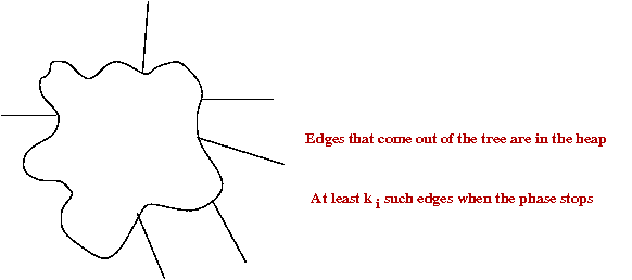
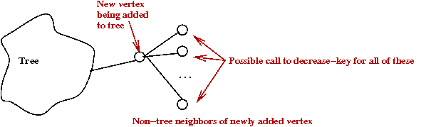
- Can we reduce the number of decrease-key operations?
- The key idea (in rough):
- Recall: when do we need decrease-key?
- Place edges into groups called "packets"
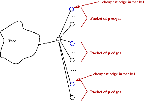
- Each packet is partially-sorted
once by edge-weight so that cheapest packet
is known.
→
One-time cost of m log(p).
- Apply decrease-key to only "packet leaders."
- Total time: O(mlog(p) + m).
- Choose p=β(m,n).
→
Total time: O(m log(β(m,n))).
Numbers big and small
Let's try and get a sense of the size of β(m,n):
- The worst case is when m = O(n2).
- Suppose n = number of atoms in the known universe (estimated).
- n = 1080 = 2266.
→
m = 2534.
→
m/n = 2266.
→
β(m,n) = 9.
→
logβ(m,n) = 4.
- Thus, logβ(m,n) = 4 for all practical purposes
in the running time of O(mlogβ(m,n)).
Exercise:
Write down (legibly) the largest number you can think of on a square-inch of paper.
Ackermann's function
[Corm2006][WP-3]:
- Consider the function
g(i) = 22 when i=1
g(i) = 2g(i-1) when i>1
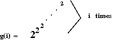
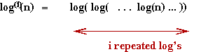
- Note:
- log(i)(n) is the inverse of g(i).
- Such a use of repeated exponentiation is called a tetration.
- Clearly, g(i) grows ridiculously fast.
- What if the tetration amount itself grows ridiculously fast?
- Now consider the function h(i) defined as:
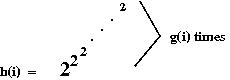
- Ackermann's function is similar, even if its definition
looks innocuous:
A(1, j) = 2j for j≥1.
A(i, 1) = A(i-1, 2) for i≥2.
A(i, j) = A(i-1, A(i,j-1)) otherwise.
- Ackermann (and co-authors) defined this to create an example
of a function that is recursive but not primitive-recursive.
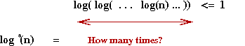
- The inverse is defined as follows:
α(m,n) = mini such that
A(i, m/n) > log(n).
- To get a sense of its size, A(4,1) > >
1080, the number of atoms in the universe.
- Thus, α(m,n) < 4 for all practical m,n.
- But theoretically, one can show that, for large enough m,n
α(m,n) < β(m,n).
- Thus, an MST algorithm that takes time
O(mα(m,n)) would be an improvement over
Gabow et al's algorithm.
On the topic of big numbers:
- Consider an integer N and Turing machines with at most n rules.
- Of these, consider those that halt.
- Of those that halt, identify the one that takes the longest
→
Takes the most steps.
- Define BB(n) = number of steps taken by the longest
halting Turing machine with at most n rules.
- Note: BB = "Busy Beaver".
- It is known that:
- BB(1) = 1.
- BB(2) = 6.
- BB(3) = 21.
→
Laborious construction and checking by hand.
- BB(4) = 107.
- So far, not so impressive.
- But, consider BB(5)
→
Not known, but it's been shown that BB(5) > 8 x 10¹⁵.
The algorithms of Chazelle and Pettie
History:
- In 1997, Bernard Chazelle
[Chaz1997]
put together the basic ideas in his new approach to MST's
that resulted in an O(m α(m,n)log(α(m,n))) algorithm.
- In 1999, both Chazelle
[Chaz2000b]
and Seth Pettie
[Pett1999]
independently improved this to O(m α(m,n)).
- In 2000, Pettie and Ramachandran
[Pett2000]
showed that, under reasonable assumptions, O(m α(m,n))
is optimal.
Because the algorithms are quite complicated (extreme!), we will
only sketch out the key ideas. There are two big innovations:
- A radically new idea for a heap data structure: the soft heap
- Achieves extract-min and decrease-key in O(1) amortized time.
- But insertion takes more time: O(log(1/ε)), where
ε is a parameter.
- The radical departure: the heap allows its contents to become
corrupted
→
The value actually changes (increases) and wrong results get
reported back.
- At most εn items are corrupted.
- This is exploited in the algorithm to tradeoff speed against
the "repair" needed to account for corruption.
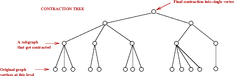
- A somewhat radically different approach to using Boruvka-phases.
- In all earlier algorithms: Boruvka phases were used
(sometimes with size-parameters) to build the tree bottom-up.
→
The contractions result in a hiearchy of components
- The "contraction tree" was useful in analysis, but not used in the algorithm.
- Here, instead, a "contraction tree" is first constructed
according to pre-specified size constraints.
- The actual MST construction uses the tree.
→
The tree is used to guide the MST-building process.
- MST construction itself occurs in separate phases.
Key ideas:
Analysis:
- The height and sub-graph sizes
of the contraction tree are under our control (as in Fredman-Tarjan).
- By choosing these carefully, the
O(mlogα(m,n)) time-bound is achieved.
Optimality:
- It can be shown that the above algorithm takes O(m)
time if m/n > O(log(3)(n))
→
i.e., it fails O(m) only for extremely-sparse graphs
(almost tree-like)
- Consider this radical idea:
- Compute MST's of all possible graphs with r vertices.
- Store these in a pre-computed look-up table.
- There are at most 2r2
such graphs.
→
(From all possible adjacency matrices)
- If r can be kept small, one can exploit this for optimality.
→
Note: r = O(log(3)(n)).
- How?
- Contract graph to reduce #vertices by factor of
O(log(3)(n)).
→
Desired density is achieved.
- Pick sub-graphs whose optimality can be immediately
determined from lookup table.
→
No cost to finding MST of these subgraphs.
- This increases the edge density to above
O(log(3)(n)).
- Now apply O(m) algorithm to remainder and join MST's.
- Two problems to address:
- How find all possible r-sized subgraphs with weights?
→
Not the same as all possible r x r binary matrices.
- How to make sure that this takes reasonable time?
- Problem 1: solve using decision-tree approach
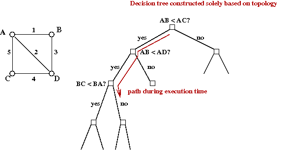
- Instead of "all possible sub-graphs", compute all possible
"decision trees on such sub-graphs".
- This is a well-known approach (in the theory world).
- Problem 2: not solved.
- Decision-tree construction time can be bound.
- But execution time depends on actual values.
→
Execution-time can't be known (or tightly bound) ahead of time.
- But, it can be shown, that it's optimal (in execution time).
→
Resulting algorithm is optimal (even if we can't pin down the
running time).
Summary
Let's step back and look at the history one more time:
- Otakar Boruvka's algorithm in 1926.
→
O(m log(n)) time (although he probably didn't know it).
→
From O(log n) phases, each requiring O(m) edge manipulations.
- Jarnik in 1930: essentially Prim's algorithm
→
O(n2) because they didn't know of heaps at
that time.
- Kruskal in 1956: O(m log(n))
→
Dominated by O(m log(m)) = O(m log(n)) sort.
- Prim in 1957: re-discovered Jarnik's algorithm
→
Still O(n2).
- Dijkstra in 1959: re-discovered Jarnik-Prim algorithm.
- The use of binary heaps: (1960's?)
- Prim + binary-heap: O(m log(n))
→
O(n log(n)) extract-min's + O(m log(n)) decrease-key's.
→
No faster than Boruvka's original algorithm (analysed in modern times).
- Improvement's to Boruvka, independently by Yao, and
Cheriton-Tarjan in 1975-76.
→
O(m loglog(n))
- Binomial heaps in 1978.
- 10 year gap.
- Fredman-Tarjan's Fibonacci heap in 1987:
→
Direct improvement of Prim's algorithm to O(nlog(n) + m).
- Fredman-Tarjan algorithm in 1987: control heap growth
→
O(mβ(m,n)).
- Gabow et al's improvement soon after:
→
O(m logβ(m,n)).
- 10 year gap.
- Chazelle's soft-heap approach in 1997
→
O(m α(m,n)logα(m,n)).
- Chazelle's and Pettie's improvements to Chazelle's approach
in 1999:
→
O(m α(m,n)).
- Pettie and Ramachandran's decision-tree algorithm and
proof of optimality in 2000.
→
Exact time unknown but at most O(m α(m,n)).
End of story? Various other interesting variations
- An O(m) randomized algorithm by Karger et al. in 1995.
- Simpler versions of the soft heap, e.g., Kaplan et al in 2009.
- The run-relaxed heap by Driscoll et al (which improves decrease-key to
O(1) worst-case).
- Faster (O(n logn) algorithms for Euclidean MST's.
References and further reading
[WP-1]
Wikipedia entry on Minimum Spanning Trees.
[WP-2]
Wikipedia entry on Otakar Boruvka.
[WP-3]
Wikipedia entry on Ackermann's function.
[Aaro]
S.Aaronson.
Who can name the biggest number?
[Boru1926]
O.Boruvka. (paper written in Czech).
[Chaz1997] B.Chazelle.
A faster deterministic algorithm for minimum spanning trees.
Symp. Foundations of Computer Science, 1997, pp.22-31.
[Chaz2000] B.Chazelle.
The soft heap: an approximate priority queue with optimal error rate.
J. ACM, 47:6, 1012-1027, Nov. 2000.
[Chaz2000b] B.Chazelle.
A Minimum Spanning Tree Algorithm with Inverse-Ackermann Type Complexity.
J. ACM, 47, 2000, pp. 1028-1047.
[Cher1976]
D.Cheriton and R.E.Tarjan.
Finding minimum spanning trees.
SIAM J.Computing, Vol. 5, 1976, pp.724-742.
[Corm2006]
T.H.Cormen, C.E.Leiserson, R.Rivest and C.Stein.
Introduction to Algorithms (2nd Edition), McGraw-Hill, 2006.
[Dixo1992]
B.Dixon, M.Rauch and R.E.Tarjan.
Verification and sensitivity analysis of minimum spanning trees in linear time.
SIAM J.Computing,
21:6, 1992, pp.1184-1192.
[Dris1988]
J.R.Driscoll, H.N.Gabow, R.Shrairman and R.E.Tarjan.
Relaxed heaps: an alternative to Fibonacci heaps with applications
to parallel computation.
Comm.ACM, 31:11, 1988, pp.1343-54.
[Eisn1997]
J.Eisner.
State-of-the-art algorithms for minimum spanning trees: A tutorial discussion.
Manuscript, University of Pennsylvania, April 1997.
[Fred1987]
M.Fredman and R.Tarjan.
Fibonacci heaps and their uses in improved network optimization
algorithms.
J. ACM, 34, 1987, pp.596-615.
[Gabo1986]
H.N.Gabow, Z.Galil, T.Spencer and R.E.Tarjan.
Efficient algorithms for finding minimum spanning trees in
undirected and directed graphs.
Combinatorica,
6:2, 1986, pp.109-122.
[Grah1985]
R.L.Graham and P.Hell.
On the history of the minimum spanning tree problem.
Annals of the History of Computing, 7, 1985, pp.43-57.
[Jarn1930]
V.Jarnik. (paper written in Czech).
[Kapl2009]
H.Kaplan and U.Zwick.
A simpler implementation and analysis of Chazelle's soft heaps.
In Proc. ACM -SIAM Symposium on Discrete Algorithms (SODA),
New York, NY, Jan 2009, pp. 477-485.
[Karg1995]
D.R.Karger, P.N.Klein and R.E.Tarjan.
A randomized linear-time algorithm to find minimum spanning
trees.
J. ACM, 42:2, March 1995, pp.321-328.
[King1995]
V.King.
A simpler minimum spanning tree verification algorithm.
Proc. Int. Workshop on Algorithms and Data Structures,
1995, pp.440-448.
[Krus1956]
J.B.Kruskal.
On the shortest spanning subtree of a graph and the traveling
salesman problem.
Proc. Am. Math. Soc., 7, 1956, pp.48-50.
[Krus1997]
J.B.Kruskal.
A reminiscence about shortest spanning trees.
Archivum Mathematicum, 1997, pp.13-14.
[Pett1999]
S.Pettie.
Finding Minimum Spanning Trees in O(m alpha(m,n)) Time.
Technical report TR-99-23, University of Texas, Austin, 1999.
[Pett2000]
S.Pettie and V.Ramachandran.
An Optimal Minimum Spanning Tree Algorithm.
J. ACM, 49:1, 2000, pp. 16-34.
[Prim1957]
R.C.Prim.
Shortest connection networks and some generalizations.
Bell Sys. Tech. J., 36, 1957, pp.362-391.
[CS153]
R.Simha.
Course notes for CS-153 (Undergraduate algorithms course).
[Weis2007]
M.A.Weiss. Data Structures and Algorithm Analysis in Java,
2nd Ed., Addison-Wesley, 2007.
[Vuil1978]
J.Vuillemin.
A data structure for manipulating priority queues.
Comm. ACM, 21:4, April 1978, pp. 309-315.
[Yao1975]
A.Yao. An O(E loglog(V)) algorithm for finding minimum spanning trees.
Inf.Proc.Lett., Vol. 4, 1975, pp.21-23.