A Dash of Physics

Relax - there will NO physics expected in the course: no homeworks, nor exams.

That said, we will describe bits and pieces of relevant physics for the curious.

The physics is itself interesting on its own, and forms useful background for those who want to go further in quantum computing.

Very little of these bits need anything more than elementary notions:

• At some point in every physics explanation, one passes from principles in physics to mathematics.
• Often this happens very quickly so, really, it's more math than physics at that point.

The highlight of physics we want to most emphasize is its vectorial nature.

Let's explain in steps:

• First, think of some object moving frictionlessly in a straight line, such as a block on ice:

  

• A block like this that moves at constant velocity keeps moving, and the velocity is $$ v \eql \frac{r(t)}{t} $$ One way to state this: the constant velocity is the total distance traveled divided by the total time, a sort of "average".

• But a slight change in scenario (block sliding down an incline) needs more to describe:

  

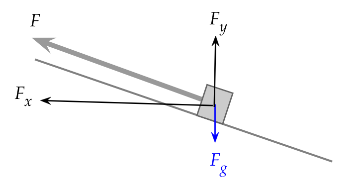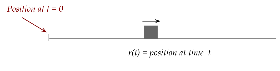
  • Experimental results (Galileo) show that the velocity increases over time as the block proceeds downwards.
  • This is where Newton made his key insight: velocity is the instantaneous rate of change of distance: $$ v(t) \eql \frac{dr(t)}{dt} \eql x^\prime(t) $$
  • And because velocity is itself changing, it's fair to ask: what is $$ a(t) \eql \frac{dv(t)}{dt}? $$

• Newton's answer: to a very good approximation, \(a(t)\) is constant.
  • This is the kind of thing that has the potential of becoming a law: nature is such that acceleration is constant.
  • A more refined theory will account for gravity that pulls objects downward and is stronger the closer you get to the bottom of the incline, meaning \(\frac{da(t)}{dt} \neq 0\).

• For this example (straight line motion), one doesn't need vectors, but let's point it out anyway:

  

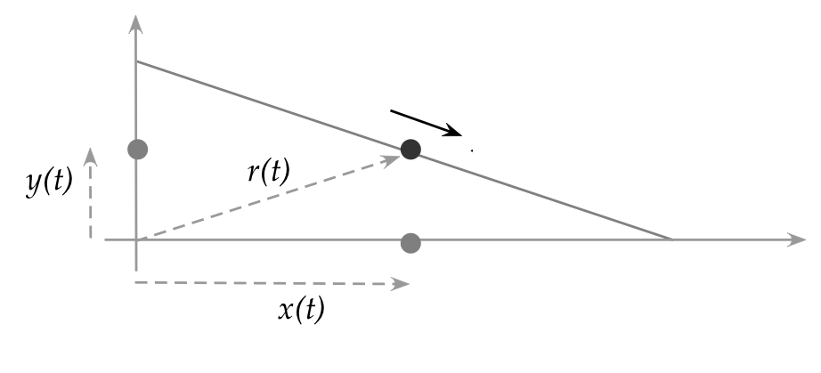
  In the vectorized version (where we've simplified the object to a point object):

  • The vector \(r(t)\) describes position.
  • Because it's a vector, it has x,y components that are also changing with time: \(r(t) = (x(t), y(t))\)
  • Suppose we observe the shadows on the x and y axes made by the object.
  • The shadows move according to \(x(t)\) and and \(y(t)\).
  • Note: \(x(t)\) and \(y(t)\) are vectors too!
  • We've called them projections along the x and y axes.

• Next, let's observe:
  • Since \(r(t), x(t), y(t)\) are vectors, we should switch to vector notation: \({\bf r}(t), {\bf x}(t), {\bf y}(t)\)
  • Vector addition gives: \({\bf r}(t) = {\bf x}(t) + {\bf y}(t)\)
    (As we would expect.)
  • Now, the differentiation operator is linear (remember?) and so $$ \frac{d{\bf r}(t)}{dt} \eql \frac{d{\bf x}(t)}{dt} + \frac{d{\bf y}(t)}{dt} $$
  • That is, the object's motion can be completely reconstructed from the motions of its shadows on the axes.
  • This holds for acceleration too.

• Thus, applying the straight-line motion laws to the shadows (projections along orthogonal directions) completely describes the motion.

• More importantly, the laws of motion can be described vectorially, exploiting vector addition when needed.

• The exact same projection approach works for curved motion, as in throwing a ball:

  

  • The power of linearity is that different rules can apply to each component.
  • Thus the \({\bf x}(t)\) motion is not impacted by gravity, but \({\bf y}(t)\) is.
  • When applying what matters to each component, one simply adds to get the actual location.

The concept of a force:

• Observation shows that accelerated motion is caused by something.

• The term force was invented to account for the something.

• Along with that, a dependence on the size and density of the object in motion (which boils down to mass, another concept).

• Thus came Newton's \(F=ma\) law: an object of mass \(m\) that experiences instantaneous force \(F\) undergoes instantaneous acceleration \(a\).

• Because the right side is a vector, so is the left side. So, we should really write this as: \({\bf F} = m \; {\bf a}\)

• This means forces can be vectorialized too, allowing for all kinds of simplification in problem-solving.

• For example, suppose our block was being pulled up the incline by a rope:

  

  • The force exerted by the rope can be projected into its x and y components as shown.
  • Gravity exerts a force, as shown in blue.
  • The overall "upward" force is the difference in the two vertical forces.

Other highlights:

• Because mass and velocity often occur as a product, it's convenient to give this a name: \(m{\bf v} \eql\) momentum.

• The symbol \({\bf p}\) is often used.

• Then one writes \({\bf F}=m{\bf a}\) as \({\bf F} = \frac{d{\bf p}}{dt}\).

• When an object moves along a curve, some force must prevent the natural tendency to move in a straightline.
  • In this case, the position vector \({\bf r}(t)\) traces out a curve over time.
  • The instantaneous force must relate, somehow, to both the instantaneous position \({\bf r}(t)\) and the instantaneous momentum \({\bf p}(t)\).
  • Combining these two produces something called angular momentum.
  • Think of angular momentum as a convenient way to describe motion along arbitrary curves.

• Another useful concept is energy:
  • Suppose we have a situation where force is changing, for example, the more you extend a spring, the more the force that wants to pull it back.
  • In this case, force changes with distance: let's say \({\bf F}(x)\) along the x direction.
  • Then, there is some function \(V(x)\) such that \(-V^\prime(x) = F(x)\).
  • This is given the name potential energy.
  • By working through the terms in motion, it turns out that to keep overall energy constant, a changing potential energy must result in a change of some other kind of energy.
  • That other kind is called kinetic energy, written as \(\frac{1}{2} m{\bf v}^2\) in terms of velocity or \(\frac{{\bf p}^2}{2m}\) in terms of momentum.