Module objectives
The main goals of this module:
- Develop the steps in reversible construction.
- Introduce binary-variable shorthand notation.
- Explore limitations of the approach.
8.1
What is reversible construction?
Let's first describe what is meant by this term at a high-level,
and then ask why it's useful.
Steps in reversible construction:
- The starting point is: a computational problem we'd
like to solve.
- Step 1: Solve the problem classically using
a classical (Boolean) circuit:
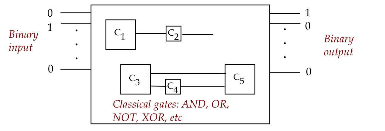
- Step 2: Replace the classical gates with
classical reversible versions:
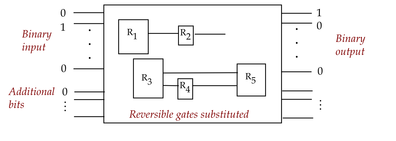
- Here, each classical gate \(C_i\) is replaced by a reversible
equivalent \(R_i\).
- The reversible ones are typically larger (more inputs and outputs).
- Step 3: Substitute quantum (reversible) equivalents of
the reversible classical gates, and use qubits:
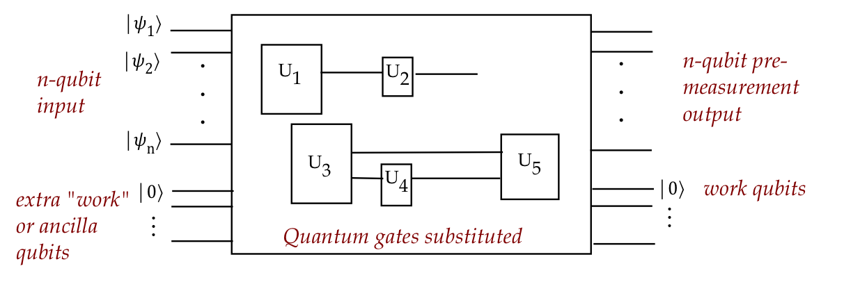
- Quantum gates are already reversible (unitaries are invertible).
- Step 4: Optionally, optimize the quantum circuit.
- Terminology: the extra "work space qubits" are often
called ancillae qubits (Singular: ancilla).
Let's ask: why construct a quantum circuit of the same size if
a classical circuit solves a problem?
- One answer: a quantum algorithm will typically
need to perform standard operations like addition
- Addition can be done efficiently in a classical circuit.
- However, itt does not make sense to transfer
qubit state (measurement!) from a quantum circuit to classical
just to perform addition.
- Instead, it's best to implement efficient classical
circuitry in a quantum circuit.
- A second answer: we can feed as input a superposition of all
standard-basis vectors:
$$
\kt{\psi_{input}}
\eql
\smf{1}{\sqrt{N}} \sum_i \kt{i}
\eql
\smf{1}{\sqrt{N}}
\parenl{ \kt{00...0} + \ldots + \kt{11...1} }
$$
- The hope is that the quantum circuit can act on all
in parallel.
- However: we need to measure at the end
- Measurement will result in only one output.
- And this too is random.
- Thus, one needs more than the reversible construction:
- Additional circuitry is needed to arrange for some desired
outputs to occur with higher probability
\(\rhd\)
Interference!
Why consider this reversibility approach?
- This is one of three high-level approaches to quantum circuit:
- Crafting circuits by hand
- Algorithmically converting a giant unitary into circuits with
as few gates as possible.
- Reversible construction.
- So far, only the first approach has been successful.
- Also, even hand-crafted quantum circuits make use
of building blocks:
- For example: an adder.
- These can be implemented via classical circuits and then optimized.
- There is on-going work in the second.
- The third, the reversible approach, at least provides
a starting point that one can further optimize.
- The reversible approach also proves that a quantum circuit
can, with low overhead, implement a classical circuit.
8.2
Binary-variable notation
It will be convenient to introduce some notational conventions
for binary variables, to be used in three situations.
First: we use them to describe Boolean gates:
- Example: the classical NOT gate
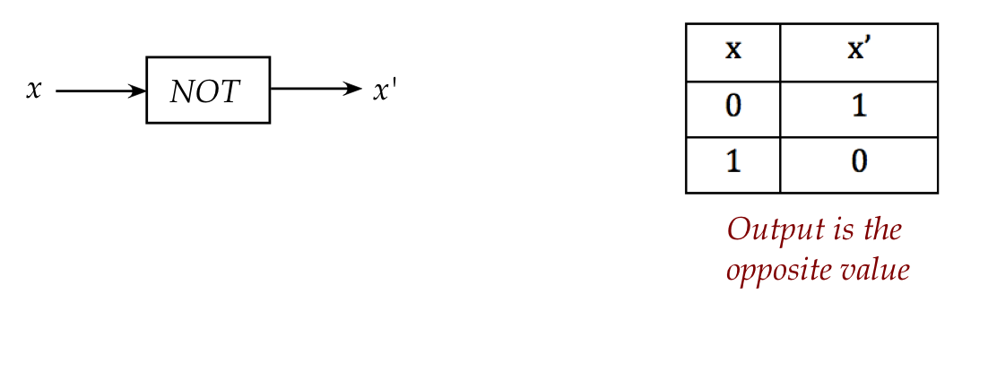
We write this as
$$
\mbox{NOT}(x) \eql x^\prime
$$
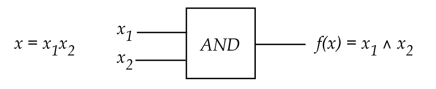
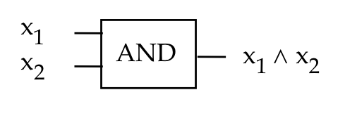
- Next, the classical AND gate:
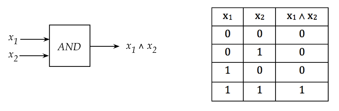
Which we write as any of
$$
\mbox{AND}(x_1,x_2) \eql x_1 \wedge x_2 \eql x_1x_2
$$
- Here, variables like \(x_1, x_2\) are binary variables
- Each \(x_i \in \{0,1\}\).
- Typically, lower case letters are used.
- The classical OR gate:
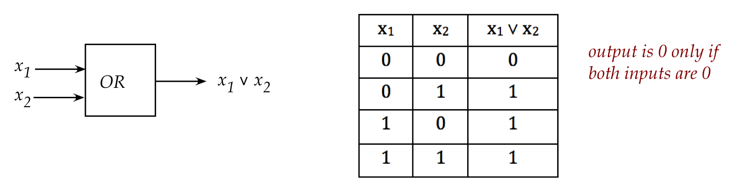
written symbolically as
$$
\mbox{OR}(x_1,x_2) \eql x_1 \vee x_2 \eql x_1 + x_2
$$
- And, an important one for us: the XOR gate
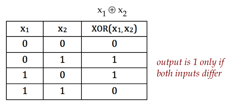
Note the XOR symbol: \(x_1 \oplus x_2\).
- A useful property that XOR shares with AND, OR:
$$
x_1 \oplus (x_2 \oplus x_3) \eql (x_1 \oplus x_2) \oplus x_3
$$
So that we can write (unambiguously): \(x_1 \oplus x_2 \oplus x_3\)
- Other useful properties:
- \(x \oplus x = 0\)
- \(x \oplus 0 = x\)
- \(x \oplus y = y \oplus x\)
The second use for binary variables is in compactly describing
quantum gates:
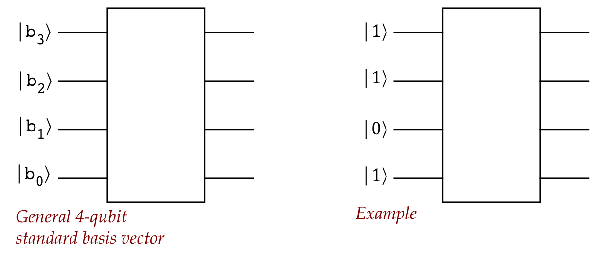
The third use of binary variables: naming bits in standard-basis vectors
- Consider the 4-qubit vector \(\kt{1101}\).
- We use the notation \(\kt{b_3 b_2 b_1 b_0}\) to describe
any 4-qubit standard-basis vector.
- Here, each \(b_i \in \{0,1\}\) is a binary variable.
- Thus, with \(b_3=1, b_2=1, b_1=0, b_0=1\), we get the
standard basis vector \(\kt{1101}\).
- In general, an n-qubit standard-basis vector can be
written as \(\kt{b_{n-1}b_{n-2} \ldots b_1 b_0}\).
- Terminology:
- The leftmost bit is called the most significant bit.
- And the rightmost, the least significant bit.
- To see why, consider how the decimal equivalent is built out
of the bits:
$$
k \eql b_{n-1} 2^{n-1} + b_{n-2} 2^{n-2} + \ldots b_1 2^1 + b_0 2^0
$$
-
For example
$$\eqb{
\kt{1101}
& \eql & \kt{b_3 2^3 + b_2 2^2 + b_1 2^1 + b_0 2^0}\\
& \eql & \kt{2^3 + 2^2 + 1} \\
& \eql & \kt{13}
}$$
- The drawing convention is to place the qubit equivalent
to the most significant bit on top:
Bitwise or binary-string operators:
- It will be useful to extend some operators to
binary strings.
- Let
$$\eqb{
b & \eql & b_{n-1} b_{n-2} \ldots b_1 b_0 \\
c & \eql & c_{n-1} c_{n-2} \ldots c_1 c_0 \\
}$$
represent two binary strings.
- Then, define:
$$\eqb{
b \wedge c & \eql & (b_{n-1} \wedge c_{n-1}) \; \ldots \; (b_0 \wedge c_0)\\
b \oplus c & \eql & (b_{n-1} \oplus c_{n-1}) \; \ldots \; (b_0 \oplus c_0)\\
}$$
- For example, suppose
$$\eqb{
b & \eql & 1011 \\
c & \eql & 1001 \\
}$$
Then
$$\eqb{
b \wedge c & \eql & (1 \wedge 1) (0 \wedge 0) (1 \wedge 0) (1 \wedge 1)
& \eql & 1 0 0 1 \\
b \oplus c & \eql & (1 \oplus 1) (0 \oplus 0) (1 \oplus 0) (1 \oplus 1)
& \eql & 0 0 1 0 \\
}$$
(Remember: each term in parentheses represents a separate binary digit.)
- And, it's also convenient to extend the real-vector dot
product to binary strings:
$$
b \cdot c \eql b_{n-1} c_{n-1} + \ldots + b_0 c_0
\eql \; \mbox{Number of common 1's}
$$
- Example:
$$
1011 \, \cdot \, 1001
\eql
(1 \cdot 1) + (0 \cdot 0) + (1 \cdot 0) + (1 \cdot 1)
\eql 2
$$
- There's a useful variation of the dot product:
$$
(b \cdot c)_2 \eql (b \cdot c) \mbox{ mod } 2
$$
- Example:
$$
(1011 \, \cdot \, 1001)_2
\eql
\parenl{ (1 \cdot 1) + (0 \cdot 0) + (1 \cdot 0) + (1 \cdot 1) }_2
\eql 2 \mbox{ mod } 2
\eql 0
$$
The binary-variable notation enables creating
useful algebraic identities, as in this example:
- Recall how we created the n-qubit all-vector equal superposition
from the all-zero input vector:
$$
\parenl{H \otimes H \otimes \ldots \otimes H}
\kt{0}\kt{0} \ldots \kt{0}
\eql
\smf{1}{\sqrt{N}} \sum_{k=0}^{N-1} \kt{k}
$$
where \(N = 2^n\) and \(k\) is decimal.
- For example,
$$\eqb{
\parenl{H \otimes H} \kt{0}\kt{0}
& \eql &
\smf{1}{\sqrt{4}} \sum_{k=0}^{3} \kt{k} \\
& \eql &
\smf{1}{\sqrt{4}} \parenl{ \kt{0} + \kt{1} + \kt{2} + \kt{3} } \\
& \eql &
\smf{1}{2} \parenl{ \kt{00} + \kt{01} + \kt{10} + \kt{11} } \\
}$$
- Sometimes, this is called the Walsh-Hadamard transform:
$$
W \eql H \otimes H \otimes \ldots \otimes H
$$
and so
$$
W\kt{00\ldots 0}
\eql
\smf{1}{\sqrt{N}} \sum_{k=0}^{N-1} \kt{k}
$$
- Although \(W\) was applied above to \(\kt{00\ldots 0}\)
we will want to see what it does to any standard-basis vector.
- Let \(k\) and \(m\) be two decimal numbers with
binary representation
$$\eqb{
k & \eql & b_{n-1} \ldots b_0 & \; \defn \; & b \\
m & \eql & c_{n-1} \ldots c_0 & \; \defn \; & c \\
}$$
where we've defined variables \(b,c\) to represent the
binary strings \(b_{n-1} \ldots b_0\) and \(c_{n-1} \ldots c_0\).
- We'll also use the terms
$$\eqb{
k & \eql & \mbox{decimal}(b)
& \mbx{Convert binary string \(b\) to decimal number \(k\)} \\
b & \eql & \mbox{binary}(k)
& \mbx{Binary string \(b\) from decimal number \(k\)} \\
}$$
- Recall that the action of \(H\) can be written as
$$
H \kt{x} \eql \isqts{1} \parenl{ \kt{0} + (-1)^x \kt{1} }
$$
where, on the left, \(\kt{x}=\kt{0}\) when \(x=0\),
and \(\kt{x}=\kt{1}\) when \(x=1\).
- Then, noting that the right side basis vectors can be
written the same way, with bit strings,
$$\eqb{
H \kt{x} & \eql & \isqts{1} \parenl{ (-1)^0\kt{0} + (-1)^{x\cdot 1} \kt{1} }\\
& \eql & \isqts{1} \parenl{ (-1)^{x\cdot 0} \kt{0} + (-1)^{x\cdot 1} \kt{1} }\\
& \eql & \isqts{1} \sum_{y=0}^{1}
(-1)^{x\cdot y} \kt{y}
}$$
Here, we introduced an additional binary variable \(y\) for the sum.
- Then,
$$\eqb{
W \kt{m}
& \eql &
W \kt{c_{n-1}} \kt{c_{n-2}} \ldots \kt{c_1} \kt{c_0}
& \mbx{Expand out the basis vector \(m\)} \\
& \eql &
W \parenl{ \kt{c_{n-1}} \otimes \ldots \otimes \kt{c_0} }
& \mbx{To clarify the tensoring} \\
& \eql &
\parenl{H \otimes \ldots \otimes H}
\parenl{ \kt{c_{n-1}} \otimes \ldots \otimes \kt{c_0} }
& \mbx{Write out \(W\)} \\
& \eql &
H \kt{c_{n-1}} \otimes \ldots \otimes H\kt{c_0}
& \mbx{Distribute each \(H\)} \\
& \eql &
\isqts{1} \parenl{\kt{0} + (-1)^{c_{n-1}}\kt{1} } \otimes \ldots \otimes
\isqts{1} \parenl{\kt{0} + (-1)^{c_{0}} \kt{1} }
&\mbx{Apply each \(H\)} \\
& \eql &
\isqts{1} \parenl{ \sum_{b_{n-1}=0}^{1} (-1)^{c_{n-1}b_{n-1}} \kt{b_{n-1}} }
\otimes \ldots \otimes
\isqts{1} \parenl{\sum_{b_{0}=0}^{1} (-1)^{c_{0}b_{0}} \kt{b_{0}} }
&\mbx{Using the result above} \\
& \eql &
\smf{1}{\sqrt{2^n}}
\sum_{b_{n-1}, \ldots , b_0}
(-1)^{{c_{n-1}} \cdot b_{n-1}} \ldots (-1)^{{c_{0}} \cdot b_{0}}
\parenl{ \kt{b_{n-1}} \otimes \ldots \otimes \kt{b_{0}} }
&\mbx{Multiply out all terms} \\
& \eql &
\smf{1}{\sqrt{N}}
\sum_{b_{n-1}, \ldots , b_0}
(-1)^{c \cdot b}
\parenl{ \kt{b_{n-1} \ldots b_{0}} }
&\mbx{Basis vector in the larger space, and \(N\defn 2^n\)} \\
& \eql &
\smf{1}{\sqrt{N}}
\sum_{k=0}^{N-1}
(-1)^{c \cdot b} \kt{k}
&\mbx{Decimal version} \\
}$$
Note: the \(b_i\)'s are introduced as binary variables, one for
each \(i\) and are then "collected" into the binary string
\(b_{n-1} \ldots b_{0}\), which then got converted to
its decimal form \(k\).
- This is useful enough to make a proposition out of it:
Proposition 8.1:
The action of the Walsh-Hadamard transform on an arbitrary
n-qubit basis vector \(\kt{m}\) is
$$
W \kt{m} \eql
\smf{1}{\sqrt{N}}
\sum_{k=0}^{N-1}
(-1)^{c \cdot b} \kt{k}
$$
where \(c=\mbox{binary}(m)\), \(b=\mbox{binary}(k)\)
and \(N=2^n\).
Application:
Many algorithms start with the full-superposition. This
result enables their analysis in later stages of an algorithm's circuit.
Finally, let's ask a question: is it enough to know what a circuit
does with standard-basis vectors?
- After all, we are using binary-variable notation for standard-basis
vectors:
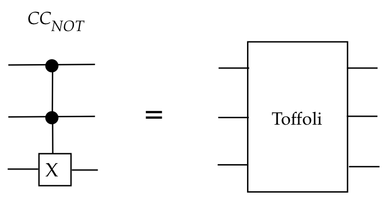
- We've described well-known gates like \(\cnot\) and Toffoli
$$\eqb{
\cnot \kt{x,y} & \eql & \kt{x, x\oplus y}\\
\mbox{TOF}\kt{x,y,z} & \eql & \kt{x,y, xy\oplus z}
}$$
- Does the action of a unitary on basis vectors completely
describe the unitary?
- Linear algebra says it clearly:
the action of any matrix (any linear transformation) is completely
determined by its action on a set of basis vectors (any basis).
- Suppose \(U\) is a matrix and \(\kt{v_1},\ldots, \kt{v_n}\)
is a basis.
- Suppose we know the list
$$
\kt{w_i} \eql U\kt{v_i}
$$
- Then, this completely determines \(U\).
- Why? Pick \(\kt{v_i}=\kt{i}\).
Then columns of \(U\) are \(U\kt{i}\) for
standard-basis vectors \(\kt{i}\).
- However, we need to be a bit careful in quantum computing
when global-phase equivalence is used.
- Consider the \(Z\) gate:
- We've seen that
$$
Z (\alpha\kt{0} + \beta\kt{1}) \eql \alpha\kt{0} + e^{i\pi} \beta\kt{1}
$$
- From which
$$\eqb{
Z \kt{0} & \eql & \kt{0} & & \\
Z \kt{1} & \eql & e^{i\pi} \kt{1} & \equiv & \kt{1} \\
}$$
(The last step uses global-phase equivalence.)
- We might be tempted to assert that \(Z\)'s action on the standard basis is:
$$\eqb{
Z \kt{0} & \eql & \kt{0} \\
Z \kt{1} & \eql & \kt{1} \\
}$$
But this would be incorrect.
(\(Z\) is not the identity)
- Thus, one must be careful when global-phase equivalence
is used in analysis.
8.3
Irreversible classical gates and their reversible replacements
In this section, we'll focus on classical gates.
In places, we'll use the conventions and tools of quantum gates
for classical gates (which at first can be a little confusing).
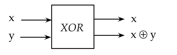
Let's use the simple XOR gate as an example:
- Consider this example output:
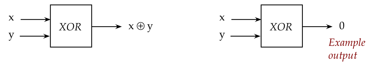
- Looking at the output (\(0\), in this case), one cannot infer the inputs:
- In contrast,
inferring the input is straightforward with the NOT gate:
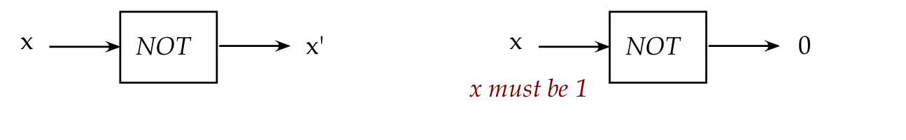
- We say that NOT is reversible while
the basic XOR-gate is not reversible.
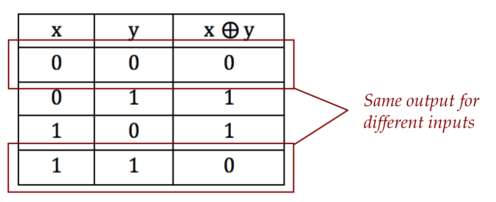
- That said, a tiny tweak makes it reversible:
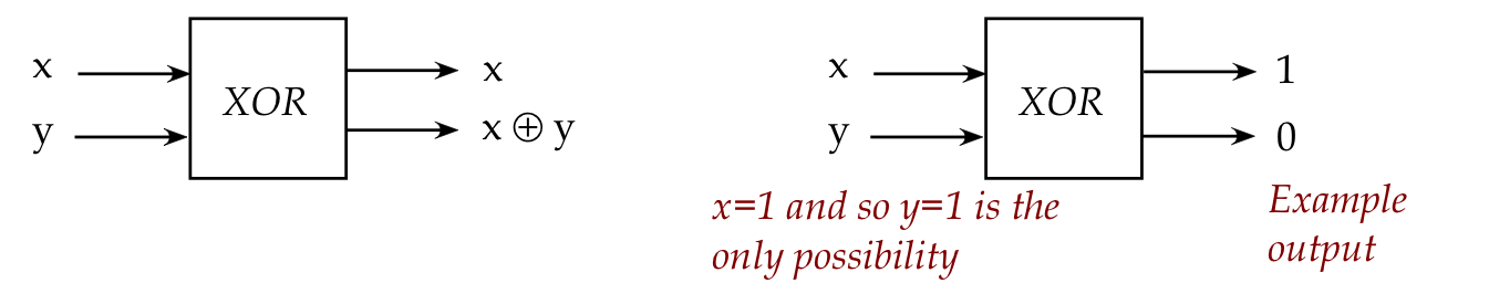
- Here, we have included one of the inputs as an output.
- Then, knowing the full output (both bits) lets us uniquely
infer the inputs.
- Let's examine the truth-table to clarify:
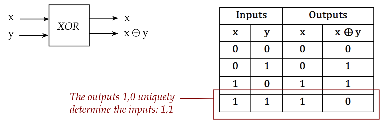
- Each pair of outputs is unique.
- Thus, the outputs uniquely determine the inputs.
- Another way of identifying reversibility: the collection of outputs
is a permutation of the inputs:

- We could call this version the XOR-with-x gate.
- We would find that XOR-with-y is also reversible.
In-Class Exercise 1:
Write out the AND-with-x and OR-with-x tables. Are these
gates reversible?
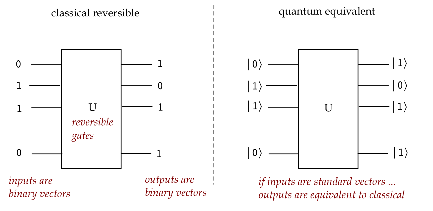
We'll now take this idea a step further:
- We know that all quantum gates are reversible:
- Any quantum gate is a unitary operation \(U\).
- And \(U\) has an inverse \(U^{-1} = U^\dagger\).
- Thus, applying \(U^\dagger\) recovers the input.
- We now ask: can we use the representation (vectors,
matrices) for quantum gates for reversible classical gates?
- Let's try this with the 2-input, 2-output XOR gate:
- The four possible inputs are \(00, 01, 10, 11\).
- With outputs \(00, 01, 10, 11\).
- Suppose we use the same vectors to represent these
that we used for \(\kt{00},\kt{01},\kt{10},\kt{11}\).
- That is:
$$
\mbox{input }00 \eql \mat{1\\ 0\\ 0\\ 0} \eql \kt{00}
\;\;\;\;\;\;\;
\mbox{input }01 \eql \mat{0\\ 1\\ 0\\ 0} \eql \kt{01}
\;\;\;\;\;\;\;
\mbox{input }10 \eql \mat{0\\ 0\\ 1\\ 0} \eql \kt{10}
\;\;\;\;\;\;\;
\mbox{input }11 \eql \mat{0\\ 0\\ 0\\ 1} \eql \kt{11}
\;\;\;\;\;\;\;
$$
- Note: with classical gates, these are the only inputs and
outputs.
There are no linear combinations or complex scalars.
- Then, what we seek is a unitary matrix such that:
$$\eqb{
\mbox{XOR} \kt{00} \eql \kt{00}
& \mbx{Outputs 0, 0}\\
\mbox{XOR} \kt{01} \eql \kt{01}
& \mbx{Outputs 0, 1}\\
\mbox{XOR} \kt{10} \eql \kt{11}
& \mbx{Outputs 1, 1}\\
\mbox{XOR} \kt{11} \eql \kt{10}
& \mbx{Outputs 1, 0}\\
}$$
- We can examine the input-to-output list above and write
out the Dirac form:
$$\eqb{
\mbox{XOR}
& \eql & \otr{00}{00} + \otr{01}{01}
+ \otr{10}{11} + \otr{11}{10} & \mbx{Binary} \\
& \eql & \otr{0}{0} + \otr{1}{1}
+ \otr{2}{3} + \otr{3}{2} & \mbx{Decimal} \\
}$$
- Alternatively, recall, we can use the sandwich approach
and compute each entry
\(\swich{i}{\mbox{XOR}}{j}\)
for \(i,j\in\{0,1,2,3\}\) (decimal).
- Either way, we get the matrix as:
$$
\mbox{XOR} \eql
\mat{
1 & 0 & 0 & 0\\
0 & 1 & 0 & 0\\
0 & 0 & 0 & 1\\
0 & 0 & 1 & 0\\
}
$$
(Which happens to be the same matrix as \(\cnot\).)
- A further insight: permutation matrices
- A permutation matrix has the property: there is only a
single 1 in every row and every column, with all other entries
being 0.
- Such a matrix permutes the elements of a vector, as in
$$
\mat{
1 & 0 & 0 & 0\\
0 & 0 & 1 & 0\\
0 & 1 & 0 & 0\\
0 & 0 & 0 & 1\\
}
\mat{a \\ b \\ c\\ d}
\eql
\mat{a \\ c \\ b\\ d}
$$
- Why is this true?
- Think of the identity matrix has having rows that
successively "act" on vector elements:
\(\rhd\)
Row \(k\) of \(I\) "picks off" element \(v_k\) in vector \({\bf v}\).
- A permutation matrix is merely a permutation of the rows of \(I\).
- Thus, if we were to use permutation matrices as classical
gates, they would perforce be reversible.
- For example: we've seen how to do this for XOR.
- Unfortunately, a 2-input solution does not exist for AND and OR.
Using Toffoli as a reversible classical gate:
- Let's borrow the Toffoli matrix from its quantum equivalent:
$$
\mbox{TOF}
\eql
\mat{
1 & 0 & 0 & 0 & 0 & 0 & 0 & 0 \\
0 & 1 & 0 & 0 & 0 & 0 & 0 & 0 \\
0 & 0 & 1 & 0 & 0 & 0 & 0 & 0 \\
0 & 0 & 0 & 1 & 0 & 0 & 0 & 0 \\
0 & 0 & 0 & 0 & 1 & 0 & 0 & 0 \\
0 & 0 & 0 & 0 & 0 & 0 & 0 & 0 \\
0 & 0 & 0 & 0 & 0 & 0 & 0 & {\bf 1} \\
0 & 0 & 0 & 0 & 0 & 0 & {\bf 1} & 0 \\
}
$$
- We already know that its effect on standard-basis
vectors can be described as:
$$
\mbox{TOF}\kt{x,y,z} \eql \kt{x,y, xy\oplus z}
$$
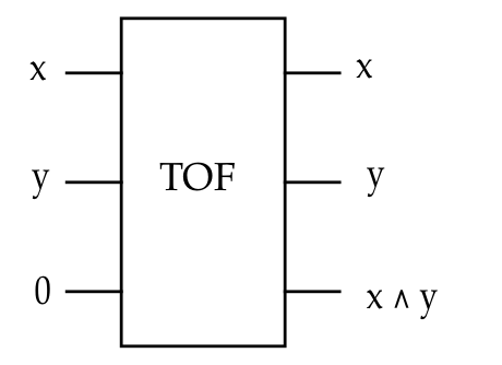
- Now observe that
$$
\mbox{TOF}\kt{x,y,0} \eql \kt{x,y, xy\oplus 0}
\eql \kt{x,y, x \wedge y}
$$
- Thus, we have a gate that can be used to compute \(x \wedge
y\), if the third input is \(0\):
- Next, a NOT-gate can be constructed as:
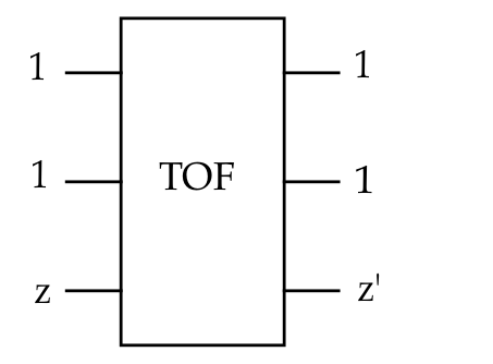
That is,
$$
\mbox{TOF}\kt{1,1,z} \eql \kt{x=1,y=1, (1\wedge 1) \oplus z}
\eql \kt{1, 1, z^\prime}
$$
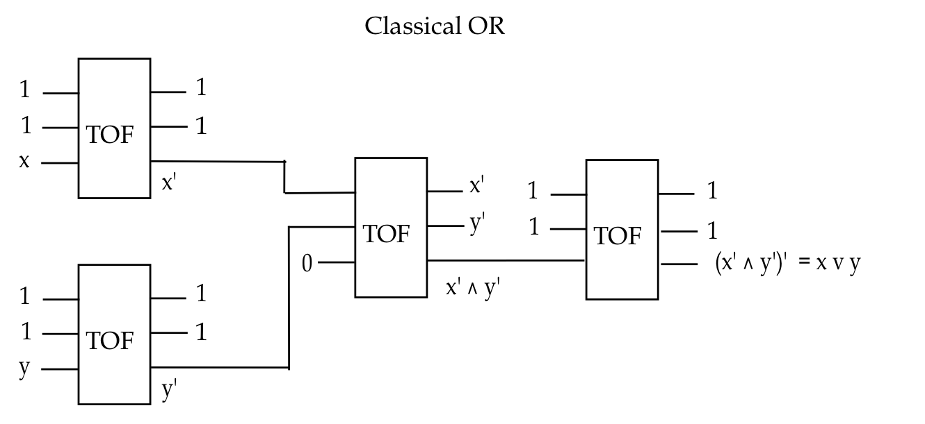
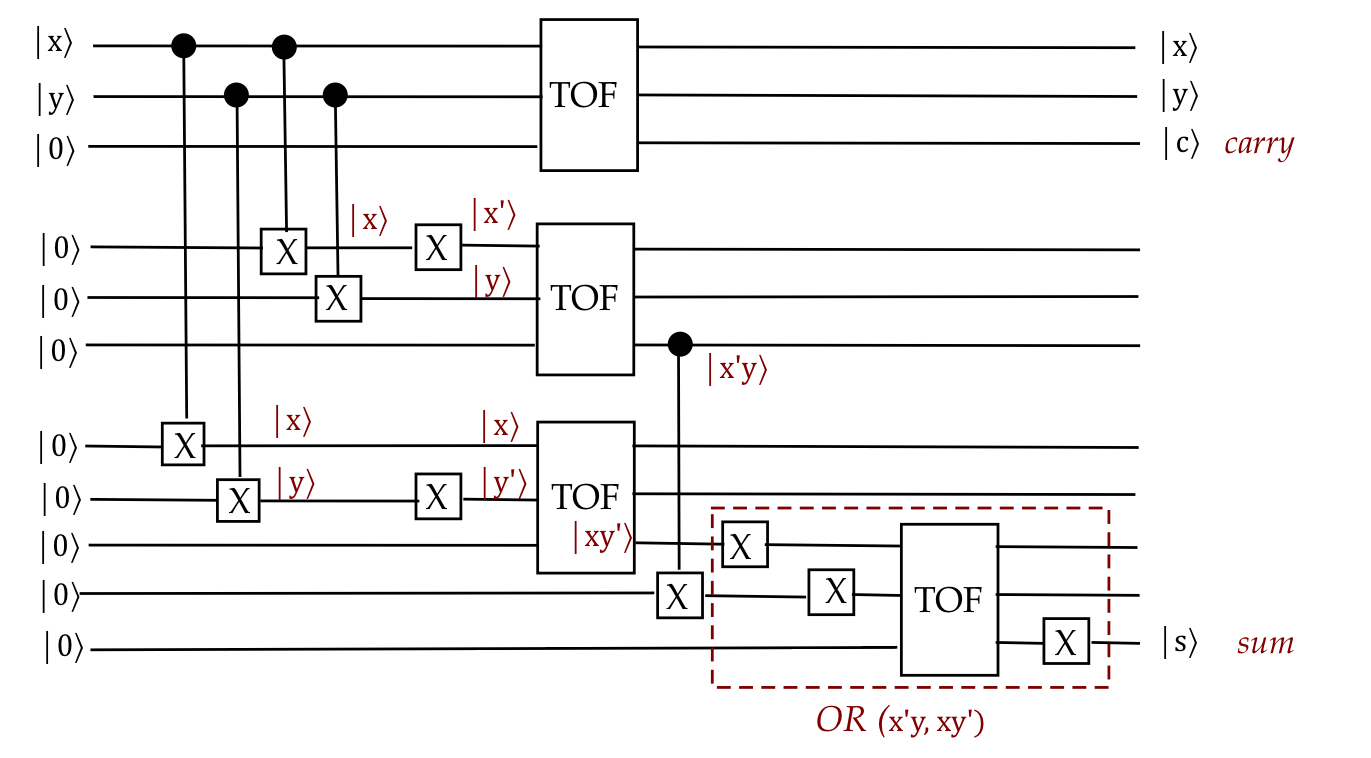
- Finally, an OR gate is more complicated:
- First,
$$
x \vee y \eql (x^\prime \wedge y^\prime)^\prime
$$
- Which we can also write as
$$
\mbox{OR}(x,y)
\eql
\mbox{NOT}\parenl{
\mbox{AND}\parenl{ \mbox{NOT}(x), \mbox{NOT}(y) }
}
$$
- Thus, working inwards
$$\eqb{
\mbox{OR}(x,y)
& \eql &
\mbox{TOF}\parenl{1, 1,
\mbox{AND}\parenl{ \mbox{NOT}(x), \mbox{NOT}(y) }
} \\
& \eql &
\mbox{TOF}\parenl{1, 1,
\mbox{TOF} \parenl{ \mbox{NOT}(x), \mbox{NOT}(y), 0 }
} \\
& \eql &
\mbox{TOF}
\parenl{ 1,1, \mbox{TOF}
\parenl{ \mbox{TOF}(1,1,x), \mbox{TOF}(1,1,y), 0}
}
}$$
- This is easier to see in a diagram:
- Thus, the Toffoli gate is universal for
classical circuits:
- Any classical circuit can be built solely out of AND and NOT
gates.
- Each such gate can be replaced by the above Toffoli
equivalents, along with extra bits.
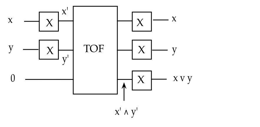
- Note, with NOT gates, one can make the Toffoli-OR circuit a bit
more efficient:
- What about these extra bits?
- The spare or extra bits are an additional cost in such an
implementation.
- In a classical circuit, they can just be discarded.
- However, this discarding cannot easily be done in a quantum
circuit because the extra bits may get entangled with the output bits.
(More about this later.)
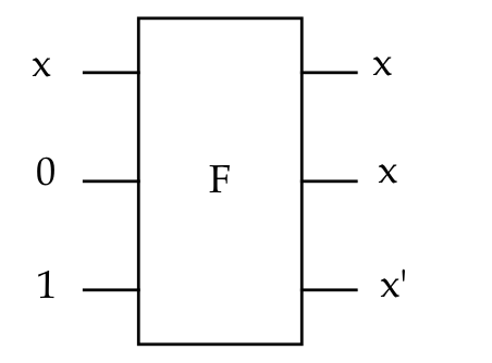
An alternative: the Fredkin or Controlled-SWAP gate
- Recall:
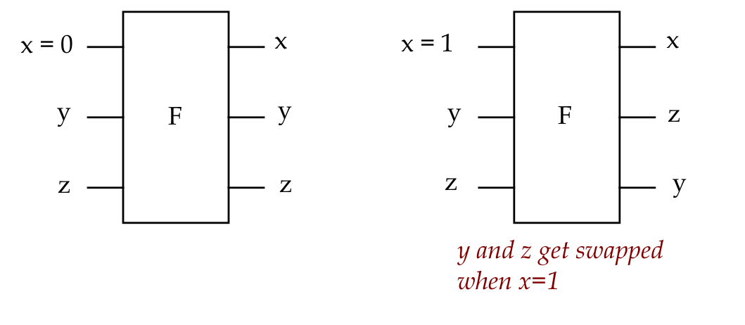
- We can write the Fredkin algebraically on standard-basis
vectors as:
$$
F \kt{x,y,z} \eql \kt{x, x^\prime y + xz, x^\prime z + xy}
$$
where \(x,y,z\) are all binary variables.
- Observe that
$$
F \kt{x,0,1} \eql \kt{x, x, x^\prime}
$$
Thus, the third output can be used as NOT(\(x\)):
- The Fredkin gate is also universal: it can implement
the NOT, AND, OR classical gates.
- Recall that the Fredkin is a controlled-SWAP and thus can
also be written as:
$$
F \kt{x,y,z} \eql (I \otimes \mbox{SWAP}^x) \kt{x,y,z}
\eql \kt{x} \otimes \mbox{SWAP}^x \kt{y,z}
$$
where \(\mbox{SWAP}^0 = I\otimes I\).
In-Class Exercise 2:
Show how the Fredkin gate can implement the classical AND and OR gates.
The meaning of the classical versions of Toffoli, Fredkin and other
such gates:
- Let's review what we know about qubits and unitary operations:
- Qubits are hardware devices that can hold a quantum state.
- A quantum state is represented mathematically by a vector.
- Qubits are modified by other hardware devices (lasers,
magnetic fields, for example).
- These modifications are mathematically represented by unitary matrices.
- Now let's review classical circuitry:
- Bits are stored in flip-flops or 1-bit registers.
- Each bit is mathematically represented by a binary variable
taking a value 0 or 1.
- Bits are modified using classical gates like AND, OR, NOT.
- These are hardware devices that take bits as input and
deliver the desired output bits.
- Classical gates are modeled by Boolean functions.
- So, what does it mean to represent classical gates
with unitary matrices?
- The idea is to simulate a classical circuit
using a quantum circuit.
- The input to the simulating quantum circuit is a
standard-basis vector.
- Then, if we use the appropriate quantum gates (with Toffoli
gates, for example), one can simulate AND and NOT.
- Then, the output vector can be interpreted
as representing a classical-circuit output.
- Note: if the input is a standard-basis
vector, the output of the simulating quantum circuit will
always be a standard-basis vector because:
- All the quantum versions of classical gates are permutations.
- Products and tensors of permutations are permutations.
(See section below.)
- After designing for standard-basis vectors as input/output,
we can of course subject a quantum circuit to superpositions, if
that suits our purpose.
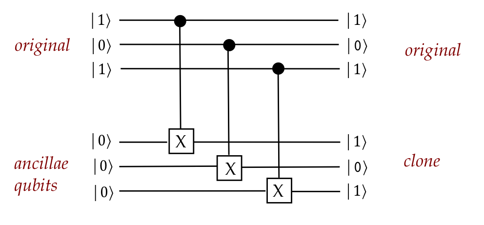
Cloning with standard basis vectors:
- While in general cloning is not possible, we can use
\(\cnot\) gates to clone standard-basis vectors, for example
8.4
An example: half-adder
Let's use a simple half-adder to contrast the procedural
classical-to-quantum approach with the hand-crafted approach.
Let's start with converting classical to quantum:
- Recall the classical half-adder:
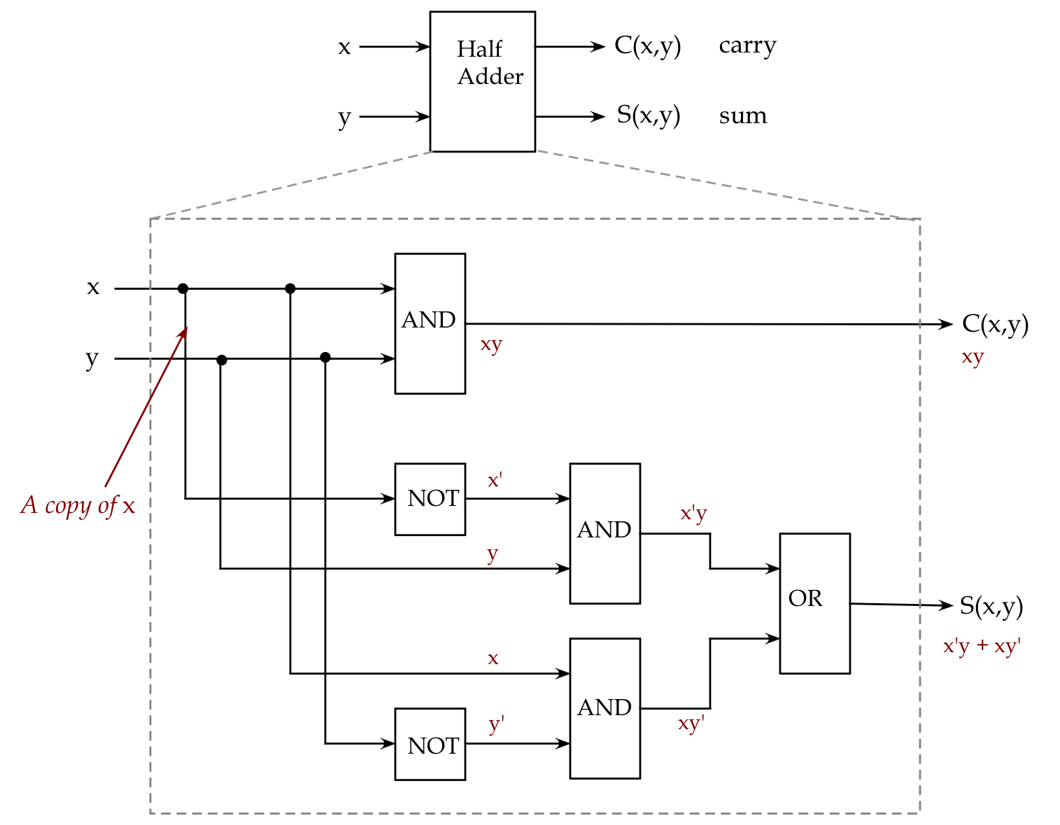
- In a purely classical circuit, copying is easy.
- In a quantum equivalent, we'll need to use \(\cnot\) gates.
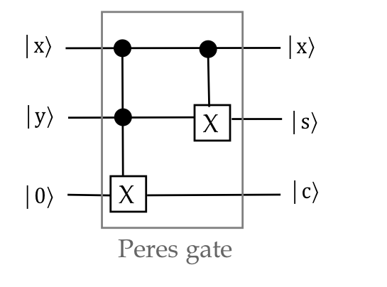
- We will build a quantum half-adder using Toffoli, NOT
and \(\cnot\) gates (for copying).
- The circuit:
Let's now contrast this with two clever hand-crafted quantum circuits:
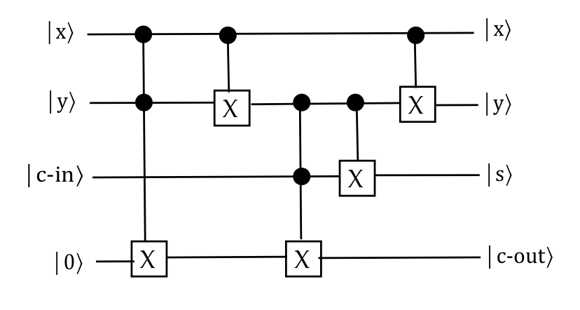
In-Class Exercise 3:
Verify that the above circuit does indeed represent
the functionality of a full adder.
8.5
Permutations and classical-to-quantum conversion
Let's examine the connection between reversible classical
circuits and permutations.
First, let's clarify what mean by a permutation.
- Let \(B_n\) be the set of length-n bit strings:
$$
B_n \eql \setl{x_{n-1} x_{n-2} \ldots x_1 x_0: x_i \in \{0,1\} }
$$
- For example:
$$
B_3 \eql \setl{000,001,010,011,100,101,110,111}
$$
- Clearly, \(|B_n| = 2^n\).
- Let \(p_n\) be a mapping from \(B_n\) to \(B_n\):
- That is, for any \(x \in B_n\),
$$
p_n (x) \; \in \; B_n
$$
- Then \(p_n\) is a permutation if it is a bijection:
$$
\forall x\neq x^\prime: \; p_n(x) \neq p_n(x^\prime)
$$
That is, for any two inputs, the corresponding outputs are different.
- One can visualize a permutation as scrambling inputs:
- Note: a permutation is not about permuting the bits
in a binary string, but permuting amongst the \(2^n\)
different binary-strings.
- Let's vectorize permutations by treating each bit string
as representing a standard-basis vector.
- For example, with \(n=2\)
$$
\kt{10} \eql \mat{0\\ 0\\ 1\\ 0}
$$
- Then, for every permutation \(p_n\) there is an
equivalent matrix \(P_n\) such that
$$
P_n \kt{x} \eql \kt{x^\prime}
\;\;\;\mbox{whenever } p_n(x) = x^\prime.
$$
- We already know how to build such a matrix using
outer-products, or the sandwich method.
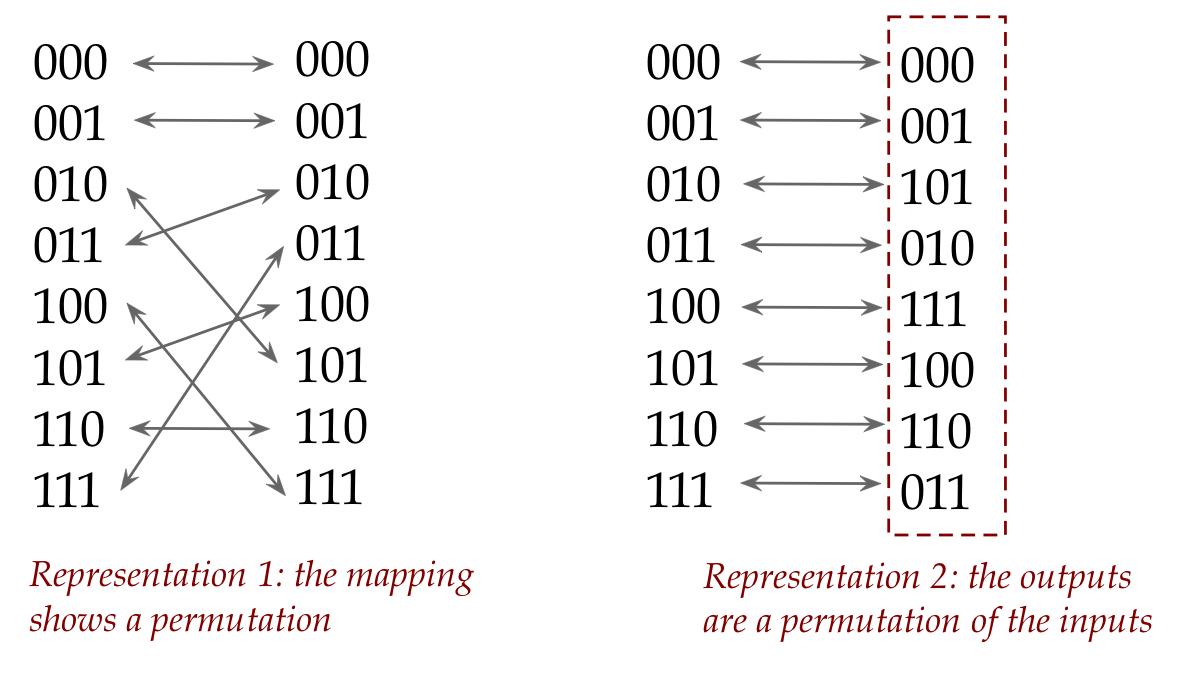
- For example, consider the permutation:
$$\eqb{
\kt{000} & \; \rightarrow \; & \kt{000} \\
\kt{001} & \; \rightarrow \; & \kt{001} \\
\kt{010} & \; \rightarrow \; & \kt{011} \\
\kt{011} & \; \rightarrow \; & \kt{010} \\
\kt{100} & \; \rightarrow \; & \kt{101} \\
\kt{101} & \; \rightarrow \; & \kt{100} \\
\kt{110} & \; \rightarrow \; & \kt{110} \\
\kt{111} & \; \rightarrow \; & \kt{111}
}$$
- The matrix is formed by the outer-product sum
$$\eqb{
P & \eql &
\otr{000}{000} + \otr{001}{001} + \otr{010}{011} +
\otr{011}{010} + \\
& &
\otr{100}{101} + \otr{101}{100} + \otr{110}{110} + \otr{111}{111}
}$$
Note: we can see the permutation by looking at the right sides
of the outer-products:
- Read the term \( \otr{100}{101}\) as "taking 101 to 100".
because
$$
\otr{100}{101} \; \kt{101} \eql \kt{100}
$$
- Writing out the matrix results in
$$
P \eql
\mat{
1 & 0 & 0 & 0 & 0 & 0 & 0 & 0 \\
0 & 1 & 0 & 0 & 0 & 0 & 0 & 0 \\
0 & 0 & 0 & 1 & 0 & 0 & 0 & 0 \\
0 & 0 & 1 & 0 & 0 & 0 & 0 & 0 \\
0 & 0 & 0 & 0 & 0 & 1 & 0 & 0 \\
0 & 0 & 0 & 0 & 1 & 0 & 0 & 0 \\
0 & 0 & 0 & 0 & 0 & 0 & 1 & 0 \\
0 & 0 & 0 & 0 & 0 & 0 & 0 & 1 \\
}
$$
- Clearly, a permutation matrix, by virtue of how we
construct it, will result in a matrix where every row and column
has only a single 1.
- Another way of thinking about a permutation matrix: it's
a permutation of the columns (rows) of \(I\).
- We have now equivalenced a reversible classical circuit
with a permutation operator.
Combining permutation operators:
- When building larger circuits from smaller ones,
we need to know:
- When two permutations occur in sequence, is the result a permutation?
- When a permutation is applied to only some qubits, is the
result a permutation of the whole?
- Proposition 8.2:
If \(P\) and \(Q\) are permutation operators, then so is \(PQ\).
Proof:
For two vectors \(\kt{x}\neq\kt{y}\), let
$$\eqb{
\kt{x^\prime} & \eql & Q\kt{x} \\
\kt{y^\prime} & \eql & Q\kt{y} \\
}$$
We know that \(Q\kt{x} \neq Q\kt{y}\) and so \(x^\prime \neq y^\prime\).
And because \(P\) is a permutation,
$$
P \kt{x^\prime} \; \neq \; P \kt{y^\prime}
$$
Hence
$$
PQ \kt{x} \; \neq \; PQ \kt{y}
$$
Intuition:
If an operator \(P\) permutes once to produce a permutation,
then permuting that permutation again (via \(Q\))
results in yet another permutation from the original.
Example:
- Suppose \(P\) permutes
$$\eqb{
\kt{00} & \; \rightarrow_P \; & \kt{01} \\
\kt{01} & \; \rightarrow_P \; & \kt{00} \\
\kt{10} & \; \rightarrow_P \; & \kt{11} \\
\kt{11} & \; \rightarrow_P \; & \kt{10} \\
}$$
and \(Q\) permutes
$$\eqb{
\kt{00} & \; \rightarrow_Q \; & \kt{11} \\
\kt{01} & \; \rightarrow_Q \; & \kt{10} \\
\kt{10} & \; \rightarrow_Q \; & \kt{01} \\
\kt{11} & \; \rightarrow_Q \; & \kt{00} \\
}$$
- Then \(PQ\) applies \(Q\) first, then \(P\):
$$\eqb{
\kt{00} & \; \rightarrow_Q \; & \kt{11}
& \; \rightarrow_P \; & \kt{10} \\
\kt{01} & \; \rightarrow_Q \; & \kt{10}
& \; \rightarrow_P \; & \kt{11} \\
\kt{10} & \; \rightarrow_Q \; & \kt{01}
& \; \rightarrow_P \; & \kt{00} \\
\kt{11} & \; \rightarrow_Q \; & \kt{00}
& \; \rightarrow_P \; & \kt{01} \\
}$$
Then the permutation \(PQ\) is:
$$\eqb{
\kt{00} & \; \rightarrow_{PQ} \; & \kt{10} \\
\kt{01} & \; \rightarrow_{PQ} \; & \kt{11} \\
\kt{10} & \; \rightarrow_{PQ} \; & \kt{00} \\
\kt{11} & \; \rightarrow_{PQ} \; & \kt{01} \\
}$$
- Proposition 8.3:
If \(P\) is a permutation operator, then so are \(I \otimes P\)
and \(P \otimes I\).
Proof:
We'll show this for \(I \otimes P\).
- Suppose \(I \otimes P\) applies to \(n\) qubits.
- Suppose \(I\) applies to the
first \(k\) qubits, and \(P\) apply to the remaining \(m\) qubits
where \(k+m = n\).
- The key is to observe that any \(n\)-qubit standard-basis
vector \(x\) is formed by tensoring lower-size vectors:
$$
\kt{x} \eql \kt{v} \otimes \kt{w}
$$
where \(\kt{v}\) is \(k\)-qubit and \(\kt{w}\) is \(m\)-qubit.
- Then for any \(w \neq w^\prime\) we are given that
$$
P\kt{w} \; \neq \; P\kt{w^\prime}
$$
- Thus
$$
(I \otimes P) \kt{v} \otimes \kt{w}
\eql
\kt{v} \otimes P\kt{w}
\; \neq \;
\kt{v} \otimes P\kt{w^\prime}
\eql
\kt{v} \otimes \kt{w^\prime}
$$
Which shows that \(I \otimes P\) is a bijection on the
standard-basis vectors.
Intuition:
- Consider the 2-qubit permutation \(P\)
$$\eqb{
\kt{00} & \; \rightarrow_P \; & \kt{01} \\
\kt{01} & \; \rightarrow_P \; & \kt{00} \\
\kt{10} & \; \rightarrow_P \; & \kt{11} \\
\kt{11} & \; \rightarrow_P \; & \kt{10} \\
}$$
- Then, \(I \otimes P\) is the 3-qubit permutation that
leaves the first bit alone:
$$\eqb{
\kt{000} & \; \rightarrow_{I\otimes P} \; & \kt{001} \\
\kt{001} & \; \rightarrow_{I\otimes P} \; & \kt{000} \\
\kt{010} & \; \rightarrow_{I\otimes P} \; & \kt{011} \\
\kt{011} & \; \rightarrow_{I\otimes P} \; & \kt{010} \\
\kt{100} & \; \rightarrow_{I\otimes P} \; & \kt{101} \\
\kt{101} & \; \rightarrow_{I\otimes P} \; & \kt{100} \\
\kt{110} & \; \rightarrow_{I\otimes P} \; & \kt{111} \\
\kt{111} & \; \rightarrow_{I\otimes P} \; & \kt{110}
}$$
Notice: the 2nd and 3rd bits are permuted according to \(P\).
- Because \(P\) is a permutation, it shuffles the right side,
resulting in a 3-qubit permutation.
What to do if a classical circuit is not a permutation:
- We already saw an example: AND
$$\eqb{
\kt{00} \; \rightarrow \; \kt{00} \\
\kt{01} \; \rightarrow \; \kt{00} \\
\kt{10} \; \rightarrow \; \kt{10} \\
\kt{11} \; \rightarrow \; \kt{11} \\
}$$
where the second bit is the binary-AND of the two input bits.
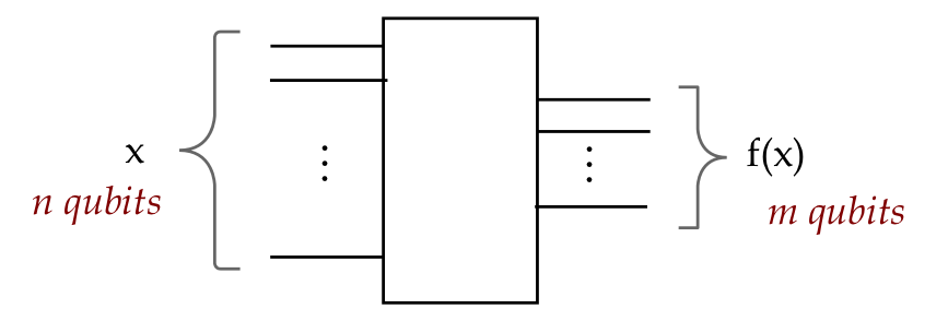
- Let \(\kt{x}\) be an n-qubit vector where \(x\) is
an n-bit string.
- Suppose \(f(x)\) is a binary-string function where
\(f(x)\) is an m-bit string.
- Typically, \(m \lt n\). Often \(m=1\) (single bit output).
- In this case \(f(x)\) cannot be a permutation.
- For example:
- Here, \(f(x) = f(x_1,x_2) = x_1 \wedge x_2\) .
- This cannot be a permutation.
- In general, with \(m \lt n\):
- That is, there exist inputs \(x\) and \(x^\prime\)
where \(f(x) = f(x^\prime)\).
There is a neat trick that equalizes the sizes of
inputs/outputs and creates a permutation:
- First, extend the input into the output:
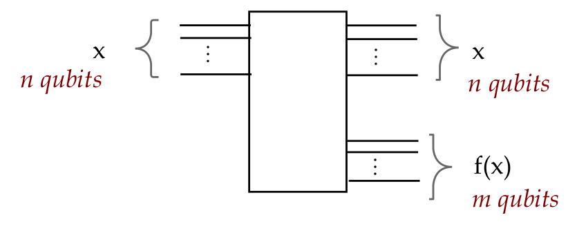
We now have an excess of outputs.
- Add additional input lines \(y\)
to match the \(m\) lines for \(f(x)\):
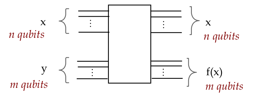
At this point, the sizes are matched but it's not clear we
have a permutation.
In fact, it's not because two different values of \(y\), keeping
\(x\) fixed, results in the same output.
- The next step is to alter the output slightly:
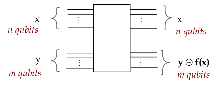
- Thus the new output is \(y \oplus f(x)\).
- Note: \(y \oplus f(x)\) performs XOR bit-by-bit for \(m\) bits.
- Since this is a classical circuit, we can easily add
additional gates to perform the bitwise XOR of
\(y\) and \(f(x)\).
- To show that this results in a permutation, we'll
show that: two different inputs result in two different outputs.
- Note:
- The input is the concatenated bit-string \(xy\).
- The output is the concatenated bit-string \(x (y \oplus f(x))\).
- Suppose \(x\) and \(x^\prime\) are different:
- Then, the inputs \(xy\) and \(x^\prime y\) are different.
- But so are \(x (y \oplus f(x))\) and \(x^\prime (y \oplus f(x^\prime))\).
- This is true even if \(f(x) = f(x^\prime)\).
- Suppose \(x = x^\prime\) and instead \(y\) and \(y^\prime\)
are the reason the inputs are different:
- Then \(y\) and \(y^\prime\) must differ in at least 1 bit.
- This will result in \(y \oplus f(x)\)
and \(y^\prime \oplus f(x)\) being different on that bit.
- Thus, the outputs will differ.
- Let's illustrate the two cases by separating out
the part that computes \(y \oplus f(x)\):
- Case 1: \(x \neq x^\prime\)
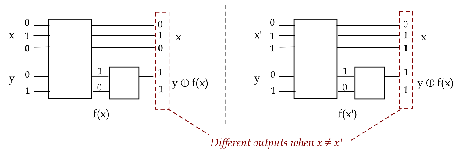
- Case 1: \(x = x^\prime, y \neq y^\prime\)
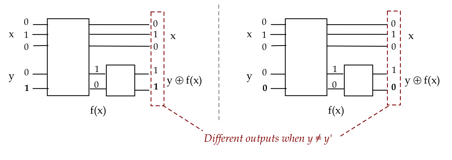
- This means the entire circuitry can be replaced by
a reversible equivalent that performs
$$
xy \; \rightarrow \; x (y \oplus f(x))
$$
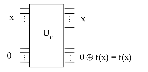
-
Which we can write vectorially as
$$
U_C \kt{x,y} \eql \kt{x, y \oplus f(x)}
$$
where \(U_C\) is the unitary (reversible) classical
permutation operator.
- However, the original goal of computing \(f(x)\) seems
thwarted: we are now computing \(y \oplus f(x)\).
- This is easily solved: when we deploy the circuit,
we simply feed \(y=00\ldots 0\) (all zeroes), so that
$$
U \kt{x,0} \eql U \kt{x, 0 \oplus f(x)}
\eql \kt{x, f(x)}
$$
That is:
- Finally, the quantum equivalent circuit is constructed
directly from the unitary matrix:
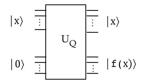
- The additional qubits are called ancilla qubits
(Plural: ancillae)
Let's work through an example with AND:
- The basic AND gate is not a permutation:
We can see this from the truthtable:
$$
\begin{array}{|c|c|c|}\hline
x_1 & x_2 & x_1 \wedge x_2 \\\hline
0 & 0 & 0 \\
0 & 1 & 0 \\
1 & 0 & 0 \\
1 & 1 & 1 \\\hline
\end{array}
$$
- Now, include \(x\) in the output and add \(y\):
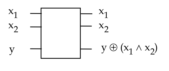
We still haven't figured out the circuit yet.
- The new truthtable is:
$$
\begin{array}{|c|c|c||c|c|c|}\hline
x_1 & x_2 & y & x_1 & x_2 & y \oplus (x_1 \wedge x_2) \\\hline
0 & 0 & 0 & 0 & 0 & 0 \\
0 & 0 & 1 & 0 & 0 & 1 \\
0 & 1 & 0 & 0 & 1 & 0 \\
0 & 1 & 1 & 0 & 1 & 1 \\
1 & 0 & 0 & 1 & 0 & 0 \\
1 & 0 & 1 & 1 & 0 & 1 \\
1 & 1 & 0 & 1 & 1 & 1 \\
1 & 1 & 1 & 1 & 1 & 0 \\\hline
\end{array}
$$
The first three columns are the inputs, the second three are outputs.
- Observe: the last three columns are a permutation (of 3-bit
bit strings).
- We can now write the input-output transformation as:
$$\eqb{
000 & \; \rightarrow \; & 000 \\
001 & \; \rightarrow \; & 001 \\
010 & \; \rightarrow \; & 010 \\
011 & \; \rightarrow \; & 011 \\
100 & \; \rightarrow \; & 100 \\
101 & \; \rightarrow \; & 101 \\
110 & \; \rightarrow \; & 111 \\
111 & \; \rightarrow \; & 110 \\
}$$
- When vectorized, this becomes:
$$\eqb{
\kt{000} & \; \rightarrow \; & \kt{000} \\
\kt{001} & \; \rightarrow \; & \kt{001} \\
\kt{010} & \; \rightarrow \; & \kt{010} \\
\kt{011} & \; \rightarrow \; & \kt{011} \\
\kt{100} & \; \rightarrow \; & \kt{100} \\
\kt{101} & \; \rightarrow \; & \kt{101} \\
\kt{110} & \; \rightarrow \; & \kt{111} \\
{\bf \kt{111}} & \; \rightarrow \; & {\bf \kt{110}} \\
}$$
- Which means the corresponding operator can be
written using a sum of outer-products:
$$\eqb{
P & \eql &
\otr{000}{000} + \otr{001}{001} + \otr{010}{010} +
\otr{011}{011} + \\
& &
\otr{100}{100} + \otr{101}{101} + {\bf \otr{110}{111}} + \otr{111}{110}
}$$
where we've highlighted one term as an example.
- In matrix form, this becomes:
$$
\mat{
1 & 0 & 0 & 0 & 0 & 0 & 0 & 0 \\
0 & 1 & 0 & 0 & 0 & 0 & 0 & 0 \\
0 & 0 & 1 & 0 & 0 & 0 & 0 & 0 \\
0 & 0 & 0 & 1 & 0 & 0 & 0 & 0 \\
0 & 0 & 0 & 0 & 1 & 0 & 0 & 0 \\
0 & 0 & 0 & 0 & 0 & 1 & 0 & 0 \\
0 & 0 & 0 & 0 & 0 & 0 & 0 & 1 \\
0 & 0 & 0 & 0 & 0 & 0 & 1 & 0 \\
}
$$
Unsurprisingly, this is the Toffoli gate or \(\ccnot\).
- In this case, the classical and quantum gates are
identical.
- In other cases, we might get a unitary permutation
that is realized in a quantum circuit using prior techniques
for decomposing a larger unitary into smaller ones.
In-Class Exercise 4:
Use the above approach to derive the outer-product form
and matrix for the unitary version of a classical OR gate.
8.6
Summary of two approaches: classical to quantum
The first approach:
- Steps:
- Build the classical circuit with ANDs and NOTs.
- Optimize classical circuit using classical techniques.
- Replace ANDs and NOTs with Toffoli gates (still classical).
- Construct the quantum circuit by using quantum Toffoli gates.
- Advantages:
- Classical-circuit optimization is well understood, and has
many algorithms.
- Works well if the quantum hardware has an efficient Toffoli gate.
The second approach:
- Steps:
- Build classical truth-table \(f(x)\) where \(x\) is
any binary string and \(f(x)\) is the binary string output.
- Convert to permutation and derive permutation (unitary)
matrix \(U_f\) such that
$$
U_f \kt{x,y} \eql \kt{x, y \oplus f(x)}
$$
- Directly optimize and construct quantum circuit.
- Advantages:
- Direct quantum circuit construction may be able to
exploit characteristics of a given quantum hardware.
- The output \(\kt{0 \oplus f(x)}\) is grouped together, making
it convenient to measure or feed into other circuits.
For the purposes of algorithm description, we'll use the latter approach.
8.7
Un-computing
Consider the additional qubits needed
in a series of unitary transformations:
- For example, consider two unitary operations \(U_1, U_2\)
in sequence:
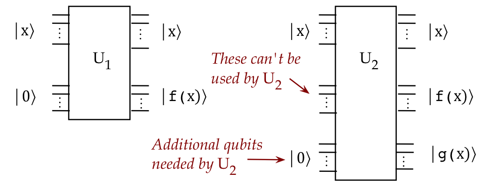
Note:
- Each of \(U_1\) and \(U_2\) need additional qubits for
reversible construction.
- \(U_2\) applies after \(U_1\).
- \(U_2\) cannot use the same qubits that \(U_1\) used as ancillae.
- Couldn't we just "reset" the ancillae qubits?
- Unfortunately, the output \(\kt{f(x)}\) could be
entangled with the input \(\kt{x}\) that is needed for \(U_2\).
- Let's tease this issue out by considering three cases.
- Consider applying \(U\) to
a 1-qubit input \(\kt{x}\), and seeing a 1-qubit output
\(\kt{f(x)}\).
- Case 1: the only input is a standard basis vector
like \(\kt{0}\) or \(\kt{1}\):
- Then, for example,
$$\eqb{
U \kt{x}\kt{0}
& \eql & U \kt{0}\kt{0}
&\mbx{Example with input \(\kt{x}=\kt{0}\)} \\
& \eql &
\kt{0, f(0)}
&\mbx{Apply \(U\) to produce \(\kt{f(x)}\) in the output}\\
& \eql &
\kt{0} \otimes \kt{f(0)}
& \mbx{The output is separable}
}$$
- Then, measuring \(\kt{f(x)}\) or resetting it has no effect
on the input, which can be used for further computations.
- Case 2: A superposition input without entanglement:
- Let's supply a superposition as the input:
$$\eqb{
U \parenl{a_0\kt{0} + a_1\kt{1}} \kt{0}
& \eql &
U \parenl{a_0\kt{0}\kt{0} + a_1\kt{1}\kt{0}}
&\mbx{Distribution of tensor over addition} \\
& \eql &
a_0 U \kt{0}\kt{0} + a_1 U \kt{1}\kt{0}
&\mbx{Linearity of \(U\)} \\
& \eql &
a_0 \kt{0, f(0)} + a_1 \kt{1, f(1)}
&\mbx{Apply \(U\) to produce \(\kt{f(x)}\)}\\
& \eql &
\parenl{a_0\kt{0} + a_1\kt{1}} \otimes \kt{f(0)}
& \mbx{Only if \(f(0)=f(1)\)}
}$$
- Again, in this special instance when \(f(0)=f(1)\),
the input is separable.
- Case 3: A superposition that results in entanglement:
- Suppose \(f(0) \neq f(1)\) and that it so happens that
\(f(0)=0, f(1)=1\).
- Then,
$$\eqb{
U \parenl{a_0\kt{0} + a_1\kt{1}} \kt{0}
& \eql &
a_0 \kt{0, f(0)} + a_1 \kt{1, f(1)}
&\mbx{Apply \(U\) to produce \(\kt{f(x)}\)}\\
& \eql &
a_0 \kt{0, 0} + a_1 \kt{1,1}
&\mbx{Entangled result}\\
}$$
- In fact, this is a type of Bell vector.
- Any measurement or resetting of the output will directly
affect the input.
- This is, after all, what the E-91 and teleportation protocols
rely on.
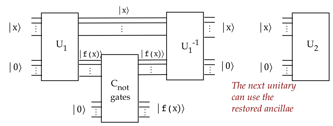
To get around this problem, the so-called uncompute trick
is used:
- First, recall that standard-basis vectors can in fact
be cloned with one \(\cnot\) per qubit cloned:
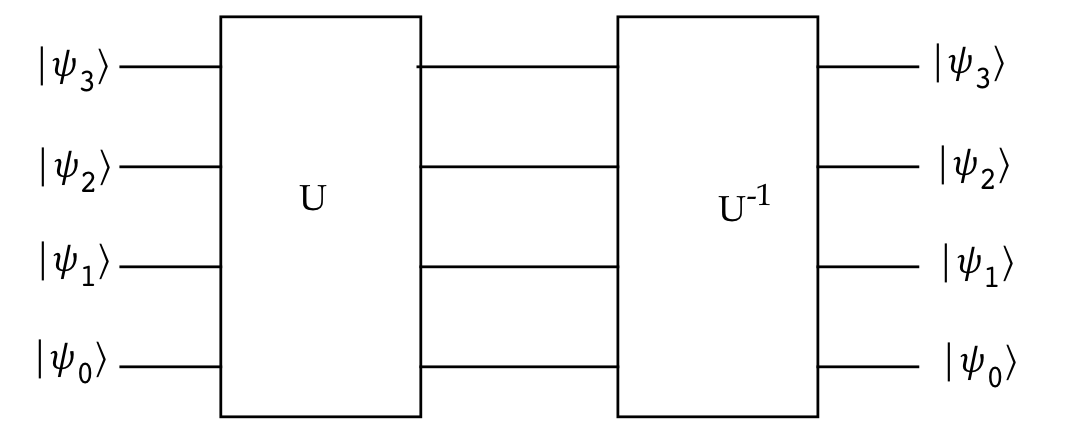
- Next, because any unitary is invertible, we can apply
the inverse to restore the original state:
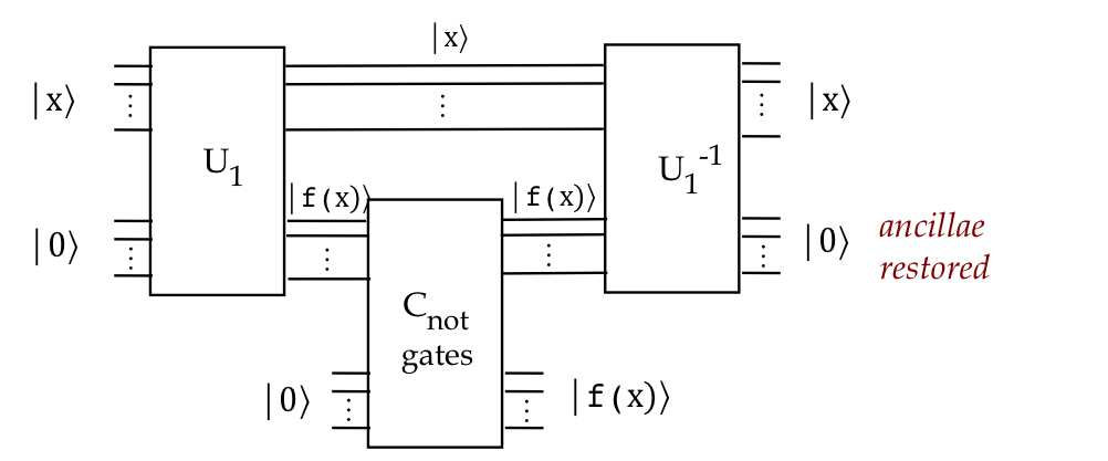
- Let's examine this idea algebraically in the
multi-qubit case first with a single multi-qubit standard-basis
vector \(\kt{x}\) as input:
- Here, \(\kt{x}\) and \(\kt{f(x)}\) are both multi-qubit.
- And \(\kt{0}\) is short for \(\kt{00\ldots 0}\).
- We'll use \(C\) to denote the entire
\(\cnot\)-based circuit.
- Now let's apply all the operators on the full set of qubits:
$$\eqb{
& \; &
\parenl{ U_1^{-1} \otimes I \otimes I} \,
\parenl{ I \otimes C} \,
\parenl{ U_1 \otimes I \otimes I} \,
\kt{x, 0, 0}
& \mbx{All three unitaries} \\
& \eql &
\parenl{ U_1^{-1} \otimes I \otimes I} \,
\parenl{ I \otimes C} \,
\kt{x, f(x), 0}
& \mbx{Apply \(U_1\), leaving the second ancillae as is} \\
& \eql &
\parenl{ U_1^{-1} \otimes I \otimes I} \,
\kt{x, f(x), f(x)}
& \mbx{\(\kt{f(x)}\) gets copied} \\
& \eql &
\kt{x, 0, f(x)}
& \mbx{\(U_1^{-1}\) restores \(\kt{0}\)} \\
& \eql &
\kt{x} \kt{0} \kt{f(x)}
& \mbx{\(\kt{0}\) is disentangled} \\
}$$
- Next, let's observe that happens when the input is
a superposition:
- In this case we'll want a general input such as
$$
\sum_x a_x \kt{x}
$$
where \(x\) is a standard-basis bit-string and
the \(a_x\)'s are coefficients.
-
$$\eqb{
& \; &
\parenl{ U_1^{-1} \otimes I \otimes I} \,
\parenl{ I \otimes C} \,
\parenl{ U_1 \otimes I \otimes I} \,
\kt{ \left(\sum_x a_x \kt{x}\right), 0, 0}
& \\
& \eql &
\parenl{ U_1^{-1} \otimes I \otimes I} \,
\parenl{ I \otimes C} \,
\parenl{ U_1 \otimes I \otimes I} \,
\parenl{\sum_x a_x \kt{x} \otimes \kt{0} \otimes \kt{0}}
& \mbx{Let's separate out the terms for clarity} \\
& \eql &
\parenl{ U_1^{-1} \otimes I \otimes I} \,
\parenl{ I \otimes C} \,
\parenl{ U_1 \otimes I \otimes I} \,
\parenl{\sum_x a_x \kt{x, 0, 0}}
& \mbx{Tensor linearity} \\
& \eql &
\parenl{ U_1^{-1} \otimes I \otimes I} \,
\parenl{ I \otimes C} \,
\parenl{\sum_x a_x (U_1 \otimes I) \kt{x, 0, 0} }
& \mbx{Linearity of \(U_1\)} \\
& \eql &
\parenl{ U_1^{-1} \otimes I \otimes I} \,
\parenl{ I \otimes C} \,
\parenl{\sum_x a_x \kt{x, f(x), 0} }
& \mbx{Apply \(U_1 \otimes I \)} \\
& \eql &
\parenl{ U_1^{-1} \otimes I \otimes I} \,
\parenl{\sum_x a_x (I\otimes C)\kt{x, f(x), 0} }
& \mbx{Operator linearity} \\
& \eql &
\parenl{ U_1^{-1} \otimes I \otimes I} \,
\parenl{\sum_x a_x \kt{x, f(x), f(x)} }
& \mbx{Apply \(\cnot\) cloning} \\
& \eql &
\parenl{\sum_x a_x (U_1^{-1} \otimes I \otimes I) \kt{x, f(x), f(x)} }
& \mbx{Operator linearity} \\
& \eql &
\sum_x a_x \kt{x, 0, f(x)}
& \mbx{Apply inverse to restore ancillae} \\
}$$
- However, because the ancillae are inside the sum, it's
not clear that they are disentangled.
- In fact, they are, although we don't have the algebraic
notation to show this.
- Let's examine the last point more closely with a
hypothetical different order, as if we had relabeled
the qubits:
- Consider
$$
\sum_x a_x \kt{x, f(x), 0}
$$
- Here, we've merely rearranged the order so that the
restored bits are written at the end.
- Now, we can easily factor out the restored ancillae:
$$
\sum_x a_x \kt{x, f(x), 0}
\eql
\sum_x a_x \parenl{ \kt{x, f(x)} \otimes \kt{0} }
\eql
\parenl{ \sum_x a_x \kt{x, f(x)}} \otimes \kt{0}
$$
Lastly, let's ask why it's important to restore the ancillae:
8.8
Efficient reversible classical circuits
Quantifiers of efficiency:
- While the actual time taken on real problems is the ultimate
measure, we need some theoretical proxies to analyze algorithms.
- Two commonly used quantifiers:
- The total number of qubits, including all ancillae and outputs.
- The number of small gates.
Let's count the added qubits needed when
converting a regular classical circuit to a reversible
equivalent:
- After all, this is the key overhead:
\(\rhd\)
If the reversible classical one is efficient, so is the quantum
equivalent.
- Let
$$\eqb{
q & \eql & \mbox{the number of classical variables or lines } \\
s & \eql & \mbox{the number of classical gates } \\
}$$
- Suppose we assume conversion from a classical non-reversible
collection of AND and NOT gates to Toffoli and NOT gates.
- Replacing each AND with a Toffoli gate needs an additional
variable (set to 0).
- In the worst-case, each of the \(s\) gates are in their own
stage, i.e., \(U_s U_{s-1} \ldots U_1\).
- In the worst-case, each stage requires as many ancillae as
the inputs, or \(q\) ancillae.
- The copying needs an additional \(q\) ancillae.
- Thus, if one did not reuse ancillae, we would need
\(2sq\) additional ancillae.
- However, by carefully reusing ancillae, one can drastically
reduce the additional ancillae needed.
- There is considerable research underway in (classical)
design-space algorithms that perform such optimizations.
Don't forget: Module-8 solved problems