Module objectives
The main goals of this module:
- Show how an arbitrary 1-qubit unitary can be implemented
with four standard gates.
- Show how an arbitrary singly-controlled 1-qubit
unitary can be implemented with seven standard gates.
- Explore how doubly-controlled unitaries can sometimes
be converted to a circuit of singly-controlled unitaries.
- Show how a multiply-controlled unitary can be expressed
in terms of doubly-controlled unitaries.
- Explain how an arbitrary n-qubit unitary can be expressed
as a circuit with multiply-controlled unitaries.
7.1
Universality: 1-qubit gates
We have seen several examples of building one gate from a combination
of others.
We now ask the question: can an arbitrary 1-qubit unitary
operation be constructed from gates we've already seen?
Let
$$
U \eql \mat{ u_{00} & u_{01}\\ u_{10} & u_{11} }
$$
be an arbitrary unitary matrix with complex numbers
\(u_{00}, u_{01}, u_{10}, u_{11}\)
We will show that one can find parameters
\(\alpha, \beta, \gamma, \delta\) such that
$$
U \eql K(\delta) \, T(\alpha) \, R(\beta) \, T(\gamma)
$$
That is,
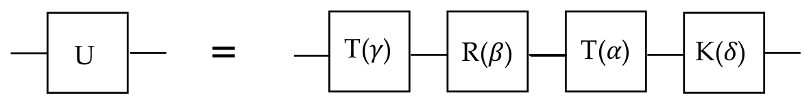
Recall:
$$\eqb{
T(\alpha)
& \eql &
e^{i\alpha Z}
& \eql &
\mat{ e^{i\alpha} & 0\\
0 & e^{-i\alpha} } \\
R(\beta)
& \eql &
e^{i\beta Y}
& \eql &
\mat{ \cos\beta & \sin\beta\\
-\sin\beta & \cos\beta} \\
K(\delta)
& \eql &
e^{i\delta I}
& \eql &
\mat{ e^{i\delta} & 0\\ 0 & e^{i\delta} }
}$$
In-Class Exercise 1:
Show that
$$
K(\delta) T(\alpha) R(\beta) T(\gamma)
\eql
\mat{ e^{i(\delta + \alpha + \gamma)} \cos\beta
& e^{i(\delta + \alpha - \gamma)} \sin\beta \\
- e^{i(\delta - \alpha + \gamma)} \sin\beta
& e^{i(\delta - \alpha - \gamma)} \cos\beta
}
$$
Let's work through the steps:
- Since \(U\) is unitary, \(U U^\dagger = I\):
$$
U U^\dagger
\eql
\mat{ u_{00} & u_{01}\\ u_{10} & u_{11} }
\mat{ u_{00}^* & u_{10}^*\\ u_{01}^* & u_{11}^* }
\eql
\mat{
u_{00}u_{00}^* + u_{01}u_{01}^* & u_{00}u_{10}^* + u_{01}u_{11}^* \\
u_{10}u_{00}^* + u_{11}u_{01}^* & u_{10}u_{10}^* + u_{11}u_{11}^*
}
$$
- Equating this to \(I\), we get four equations:
$$\eqb{
\magsq{u_{00}} + \magsq{u_{01}} & \eql & 1 \\
\magsq{u_{10}} + \magsq{u_{11}} & \eql & 1 \\
u_{00}u_{10}^* + u_{01}u_{11}^* & \eql & 0 \\
u_{10}u_{00}^* + u_{11}u_{01}^* & \eql & 0 \\
}$$
- From the third:
$$\eqb{
& \; &
u_{00}u_{10}^* & \eql & - u_{01}u_{11}^* \\
& \implies &
\magsq{u_{00}} \magsq{u_{10}} & \eql & \magsq{u_{01}} \magsq{u_{11}}
}$$
- In this, substitute
\(\magsq{u_{01}} = 1 - \magsq{u_{00}}\)
and
\(\magsq{u_{10}} = 1 - \magsq{u_{11}}\)
from the first two of the set of four equations earlier.
- This results in \(\magsq{u_{00}} = \magsq{u_{11}}\)
- A similar substitution in the fourth equation results in
\(\magsq{u_{01}} = \magsq{u_{10}}\)
- We conclude:
$$\eqb{
\mag{u_{00}} & \eql & \mag{u_{11}} \\
\mag{u_{01}} & \eql & \mag{u_{10}} \\
}$$
- Now, from the first two of earlier set of four, each
\(\mag{u_{ij}} \leq 1\).
- For any complex \(z=re^{i\theta}\) such that \(\mag{z} \leq
1\), we have \(r \leq 1\).
- This means we can find some \(\beta\) such that
\(r = \cos\beta\).
- Thus, we can write, for example:
$$
u_{00} \eql e^{i\theta_{00}} \cos\beta
$$
- Then, because \(\magsq{u_{00}} = \magsq{u_{11}}\)
$$
u_{11} \eql e^{i\theta_{11}} \cos\beta
$$
for some \(\theta_{11}\).
- Note:
- We can't conclude \(\theta_{00}=\theta_{11}\)
from \(\mag{u_{00}} = \mag{u_{11}}\).
- We can choose whether to use \(\cos\beta\)
or \(-\cos\beta\). Both work.
- Since \(\magsq{u_{01}} = 1 - \magsq{u_{00}}\),
$$
\magsq{u_{01}} \eql 1 - \magsq{u_{00}}
\eql 1 - \cos^2 \beta
\eql \sin^2\beta
$$
Thus, either \(\sin\beta\) or \(-\sin\beta\) could be used
in writing
$$
u_{01} \eql e^{i\theta_{01}} \sin\beta
$$
- Putting it all together, \(U\) can be written as
$$
\mat{ u_{00} & u_{01}\\ u_{10} & u_{11} }
\eql
\mat{
e^{i\theta_{00}}\cos\beta & e^{i\theta_{01}}\sin\beta \\
-e^{i\theta_{10}}\sin\beta & e^{i\theta_{11}}\cos\beta
}
$$
- Now equate \(U=K(\delta) T(\alpha) R(\beta) T(\gamma)\):
$$
\mat{
e^{i\theta_{00}}\cos\beta & e^{i\theta_{01}}\sin\beta \\
-e^{i\theta_{10}}\sin\beta & e^{i\theta_{11}}\cos\beta
}
\eql
\mat{ e^{i(\delta + \alpha + \gamma)} \cos\beta
& e^{i(\delta + \alpha - \gamma)} \sin\beta \\
- e^{i(\delta - \alpha + \gamma)} \sin\beta
& e^{i(\delta - \alpha - \gamma)} \cos\beta
}
$$
- This results in equations:
$$\eqb{
\delta + \alpha + \gamma & \eql & \theta_{00} \\
\delta + \alpha - \gamma & \eql & \theta_{01} \\
\delta - \alpha + \gamma & \eql & \theta_{10} \\
\delta - \alpha - \gamma & \eql & \theta_{11} \\
}$$
- We have four equations in three variables, which looks
over-constrained, but there is linear dependence:
\(\rhd\)
Only the first three are needed.
- To see why, consider the fourth of the original set of four
equations in the elements of \(U\):
$$
u_{10}u_{00}^* + u_{11}u_{01}^* \eql 0
$$
Substituting from the newly formed matrix, this gives
$$
-e^{i\theta_{10}}\sin\beta e^{-i\theta_{00}}\cos\beta
+ e^{i\theta_{11}}\cos\beta e^{-i\theta_{01}}\sin\beta
\eql 0
$$
From which
$$
e^{i(\theta_{11} - \theta_{01})}
\eql
e^{i(\theta_{10} - \theta_{00})}
$$
and thus
$$
\theta_{11} - \theta_{01} \eql \theta_{10} - \theta_{00}
$$
That is, one of the \(\theta\)'s can be expressed in terms
of the other three.
- Thus, in solving the equations, we must use only three of them.
- The parameters \(\alpha, \beta, \gamma, \delta\)
can now be chosen to create any unitary operation.
- For example, with \(\alpha=\gamma=0, \beta=\delta=\frac{\pi}{2}\),
$$
\mat{ e^{i(\delta + \alpha + \gamma)} \cos\beta
& e^{i(\delta + \alpha - \gamma)} \sin\beta \\
- e^{i(\delta - \alpha + \gamma)} \sin\beta
& e^{i(\delta - \alpha - \gamma)} \cos\beta }
\eql
\mat{ 0 & e^0 \sin\frac{\pi}{2} \\
- e^{i\pi} \sin\frac{\pi}{2} & 0}
\eql
\mat{ 0 & 1\\ 1 & 0}
\eql X
$$
In-Class Exercise 2:
What parameter values for \(\alpha, \beta, \gamma, \delta\)
result in the Hadamard gate?
7.2
Universality: controlled-U
Once a particularly useful unitary \(U\) is found, one would like to
turn it on or off as needed
\(\rhd\)
That is, design a Controlled-\(U\) in terms of the same basic
gates \(K(\delta), T(\alpha), R(\beta)\):
Recall:
$$\eqb{
K(\delta)
& \eql &
e^{i\delta I}
& \eql &
\mat{ e^{i\delta} & 0\\ 0 & e^{i\delta} } \\
T(\alpha)
& \eql &
e^{i\alpha Z}
& \eql &
\mat{ e^{i\alpha} & 0\\
0 & e^{-i\alpha} } \\
R(\beta)
& \eql &
e^{i\beta Y}
& \eql &
\mat{ \cos\beta & \sin\beta\\
-\sin\beta & \cos\beta} \\
}$$
We will also need at least one Controlled gate, for which
we'll prefer to use \(\cnot\)
Thus, the gate set we wish to use consists of:
$$
\cnot, \; K(\delta), \; T(\alpha), \; R(\beta)
$$
The starting point is a general \(U\) in the form
$$
U \eql K(\delta) T(\alpha) R(\beta) T(\gamma)
$$
as shown in the previous section.
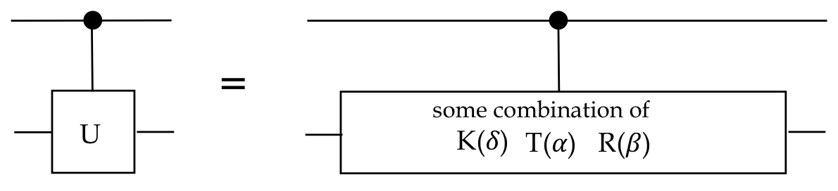
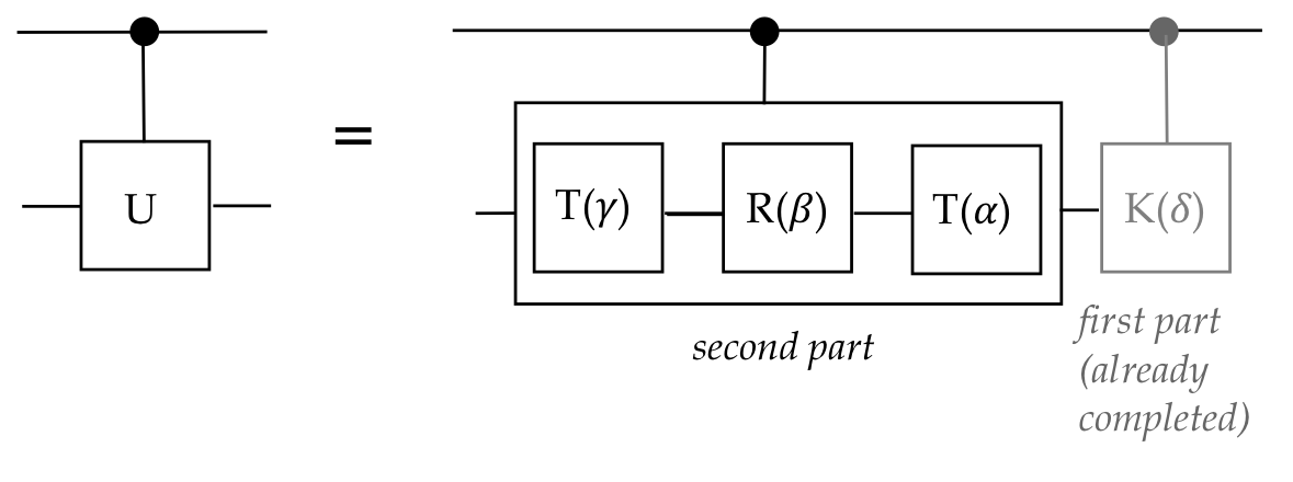
- First, we'll decompose Controlled-\(U\) into two parts:
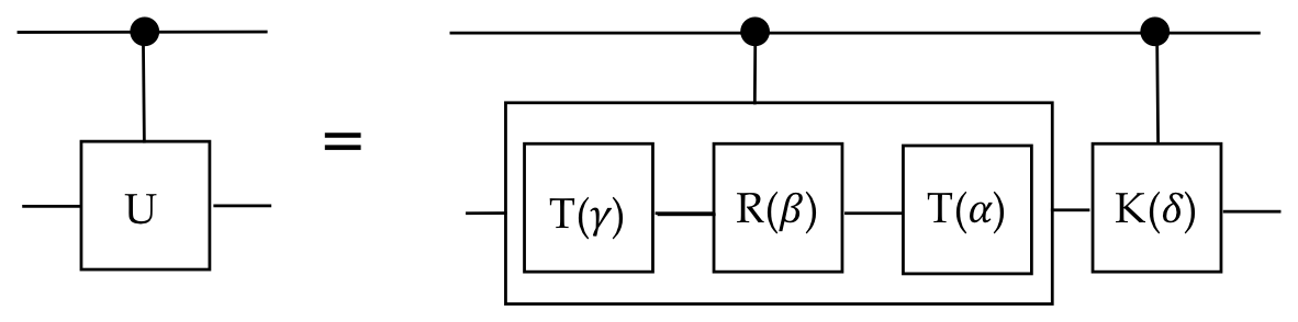
What we seek is:
- With \(\kt{0}\) as the control bit, neither unit is activated.
- With \(\kt{1}\), both are, and the resulting unitary on
the second qubit should be
$$
\parenl{ K(\delta) } \;\; \parenl{ T(\alpha) R(\beta)
T(\gamma) }
$$
We now focus on the first part of the unitary product (last to act in
the circuit):
- Recall the Dirac version of \(\cnot\):
$$
\cnot \eql \otr{0}{0} \otimes I \; + \; \otr{1}{1} \otimes X
$$
The intuition:
- When the control (first) qubit is \(\kt{0}\), apply \(I\) to
the second qubit.
- When the control is \(\kt{1}\), apply \(X\).
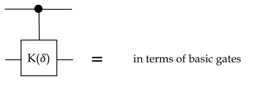
- Then, Controlled-\(K(\delta)\) can be written as:
$$
\mbox{Controlled}-K(\delta)
\eql \otr{0}{0} \otimes I \; + \; \otr{1}{1} \otimes K(\delta)
$$
- Since \(K(\delta) = e^{i\delta} I\),
$$\eqb{
\mbox{Controlled}-K(\delta)
& \eql &
\otr{0}{0} \otimes I \; + \; \otr{1}{1} \otimes K(\delta)
& \\
& \eql &
\otr{0}{0} \otimes I \; + \; \otr{1}{1} \otimes e^{i\delta} I
& \mbx{Definition of \(K(\delta)\)} \\
& \eql &
\otr{0}{0} \otimes I \; + \; e^{i\delta} \otr{1}{1} \otimes I
& \mbx{Bilinearity: constants can switch places in tensor} \\
& \eql &
\parenl{ \otr{0}{0} + e^{i\delta} \otr{1}{1} } \otimes I
& \mbx{Additivity of tensoring} \\
}$$
Recall: \(\alpha \kt{v} \otimes \kt{w} = \kt{v} \otimes \alpha \kt{w}\).
- Continuing with the first term,
$$\eqb{
\otr{0}{0} + e^{i\delta} \otr{1}{1}
& \eql &
\mat{1 & 0\\ 0 & 0} + \mat{0 & 0\\ 0 & e^{i\delta}} \\
& \eql &
\mat{e^0 & 0\\ 0 & e^{i\delta}} \\
& \eql &
\mat{
e^{-i\frac{\delta}{2}} e^{i\frac{\delta}{2}} & 0\\
0 & e^{i\frac{\delta}{2}} e^{i\frac{\delta}{2}}
} \\
& \eql &
\mat{
e^{i\frac{\delta}{2}} & 0\\
0 & e^{i\frac{\delta}{2}}
}
\mat{
e^{-i\frac{\delta}{2}} & 0\\
0 & e^{i\frac{\delta}{2}}
} \\
& \eql &
K(\sml{\frac{\delta}{2}}) T(-\sml{\frac{\delta}{2}})
}$$
- Thus, substituting,
$$\eqb{
\mbox{Controlled}-K(\delta)
& \eql &
\parenl{ \otr{0}{0} + e^{i\delta} \otr{1}{1} } \otimes I \\
& \eql &
K(\frac{\delta}{2}) T(-\frac{\delta}{2}) \otimes I
}$$
Note: the first part acts on the first qubit, and \(I\) acts on the second.
- Let's draw this part of the circuit to see something
surprising:
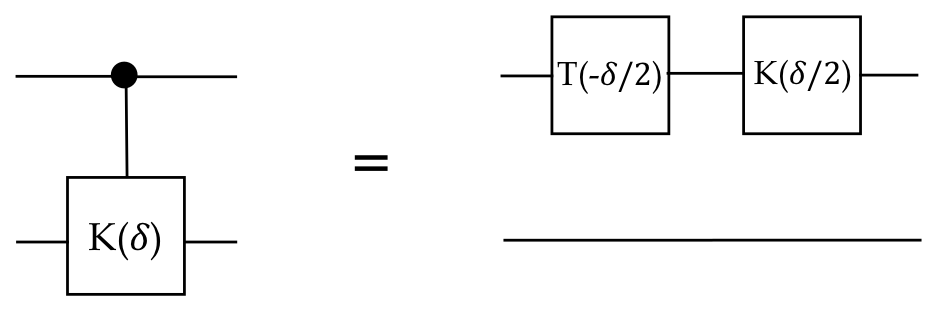
- The second qubit, the one that is controlled, passes by untouched!
- This is an unusual case in that \(K(\delta) = e^{i\delta} I\)
is really multiplication by the constant \(e^{i\delta}\).
- In a tensor, as we've seen, the constant can be moved between
tensor terms.
- Thus, for example,
$$
A \otimes e^{i\delta} I \eql e^{i\delta} A \otimes I
$$
which makes it appear that the second qubit is untouched.
- What's important to realize is that the operation is on
a 2-qubit state, which can shuffle constants between its constituents.
Next, let's turn to the second part of the overall decomposition:
The following results will be useful:
$$\eqb{
T(0) & \eql & I \\
R(0) & \eql & I \\
T(\alpha_1 + \alpha_2)
& \eql & T(\alpha_1) T(\alpha_2) \\
R(\beta_1 + \beta_2)
& \eql & T(\beta_1) T(\beta_2) \\
X \, R(\beta) \, X & \eql & R(-\beta) \\
X \, T(\alpha) \, X & \eql & T(-\alpha) \\
}$$
In-Class Exercise 3:
The first four were shown earlier.
Prove the latter two using matrix representations.
Next, let's work through the remaining steps:
- Define the following unitary combinations:
$$\eqb{
U_1 & \eql & T(\alpha) \, R(\sml{\frac{\beta}{2}}) \\
U_2 & \eql & R(-\sml{\frac{\beta}{2}}) \, T(-\sml{\frac{\gamma+\alpha}{2}}) \\
U_3 & \eql & T(\sml{\frac{\gamma-\alpha}{2}})
}$$
- Then, the product of these is
$$\eqb{
U_1 U_2 U_3
& \eql &
T(\alpha) \, R(\sml{\frac{\beta}{2}}) \,
R(-\sml{\frac{\beta}{2}}) \, T(-\sml{\frac{\gamma+\alpha}{2}}) \,
T(\sml{\frac{\gamma-\alpha}{2}})
& \\
& \eql &
T(\alpha) \, R(0) \,
T(-\sml{\frac{\gamma}{2}} - \sml{\frac{\alpha}{2}}) \,
T(\sml{\frac{\gamma-\alpha}{2}}) \\
& \eql &
T(\alpha) \,
T(-\sml{\frac{\gamma}{2}}) \, T(- \sml{\frac{\alpha}{2}}) \,
T(\sml{\frac{\gamma}{2}}) \, T(- \sml{\frac{\alpha}{2}}) \\
& \eql &
T(-\sml{\frac{\gamma}{2}}) \,T(\sml{\frac{\gamma}{2}}) \,
T(\alpha) \, T(- \sml{\frac{\alpha}{2}}) \, T(- \sml{\frac{\alpha}{2}})\\
& \eql &
T(0) \, T(0) \\
& \eql &
I
}$$
- Now consider the product \(U_1\, X\, U_2\, X\, U_3\),
with \(X\) interleaved:
$$\eqb{
U_1\, X\, U_2\, X\, U_3
& \eql &
T(\alpha) \, R(\sml{\frac{\beta}{2}}) \, X \,
R(-\sml{\frac{\beta}{2}}) \, T(-\sml{\frac{\gamma+\alpha}{2}}), \, X \,
T(\sml{\frac{\gamma-\alpha}{2}})
& \mbx{Definitions of \(U_i\)} \\
& \eql &
T(\alpha) \, R(\sml{\frac{\beta}{2}}) \, X \,
R(-\sml{\frac{\beta}{2}}) \, X^2 \, T(-\sml{\frac{\gamma+\alpha}{2}}) \, X \,
T(\sml{\frac{\gamma-\alpha}{2}})
& \mbx{\(X^2 = I\)} \\
& \eql &
T(\alpha) \, R(\sml{\frac{\beta}{2}}) \,
\parenl{ X R(-\sml{\frac{\beta}{2}}) X}\,
\parenl{ X T(-\sml{\frac{\gamma+\alpha}{2}}) X} \,
T(\sml{\frac{\gamma-\alpha}{2}})
& \mbx{Writing \(X^2 = XX\)} \\
& \eql &
T(\alpha) \, R(\sml{\frac{\beta}{2}}) \,
\parenl{ R(\sml{\frac{\beta}{2}})}\,
\parenl{ T(\sml{\frac{\gamma+\alpha}{2}})} \,
T(\sml{\frac{\gamma-\alpha}{2}})
& \mbx{From exercise above} \\
& \eql &
T(\alpha) \, R(\beta) \, T(\gamma)
}$$
This is the second part of the overall decomposition.
- Let's summarize so far:
$$\eqb{
U_1 U_2 U_3
& \eql &
I \\
U_1\, X\, U_2\, X\, U_3
& \eql &
T(\alpha) \, R(\beta) \, T(\gamma)
}$$
where each \(U_i\) is constructed with basic gates \(T(\alpha), R(\beta), K(\delta)\).
- Now consider the circuit
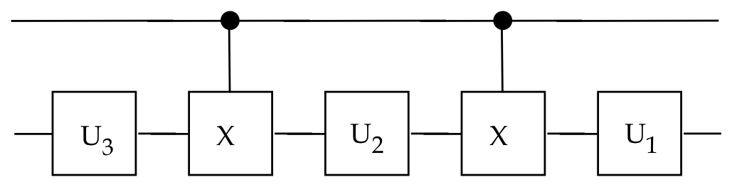
- With the control qubit as \(\kt{0}\):
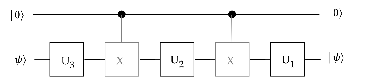
There's no change because we showed that \(U_1 U_2 U_3 = I\).
- With the control qubit as \(\kt{1}\):
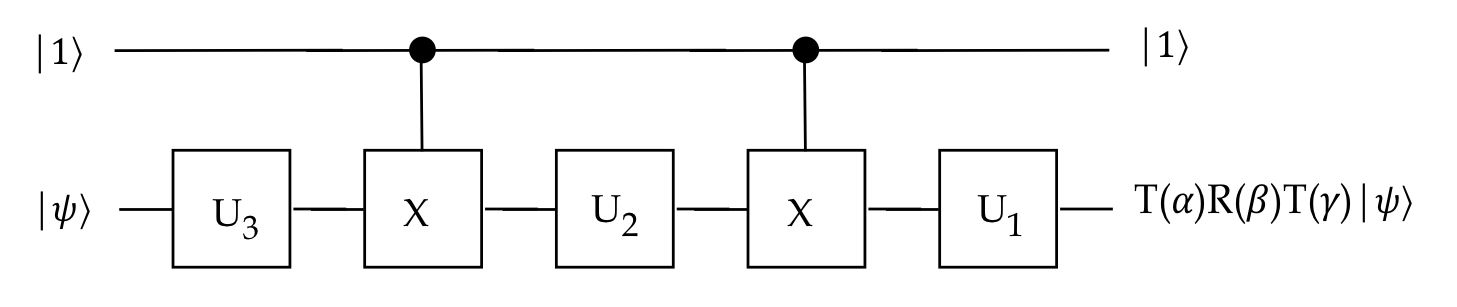
We obtain the second part of the overall decomposition:
\(U_1\, X\, U_2 X\, U_3 = T(\alpha) \, R(\beta) \, T(\gamma)\)
- Putting it all together:
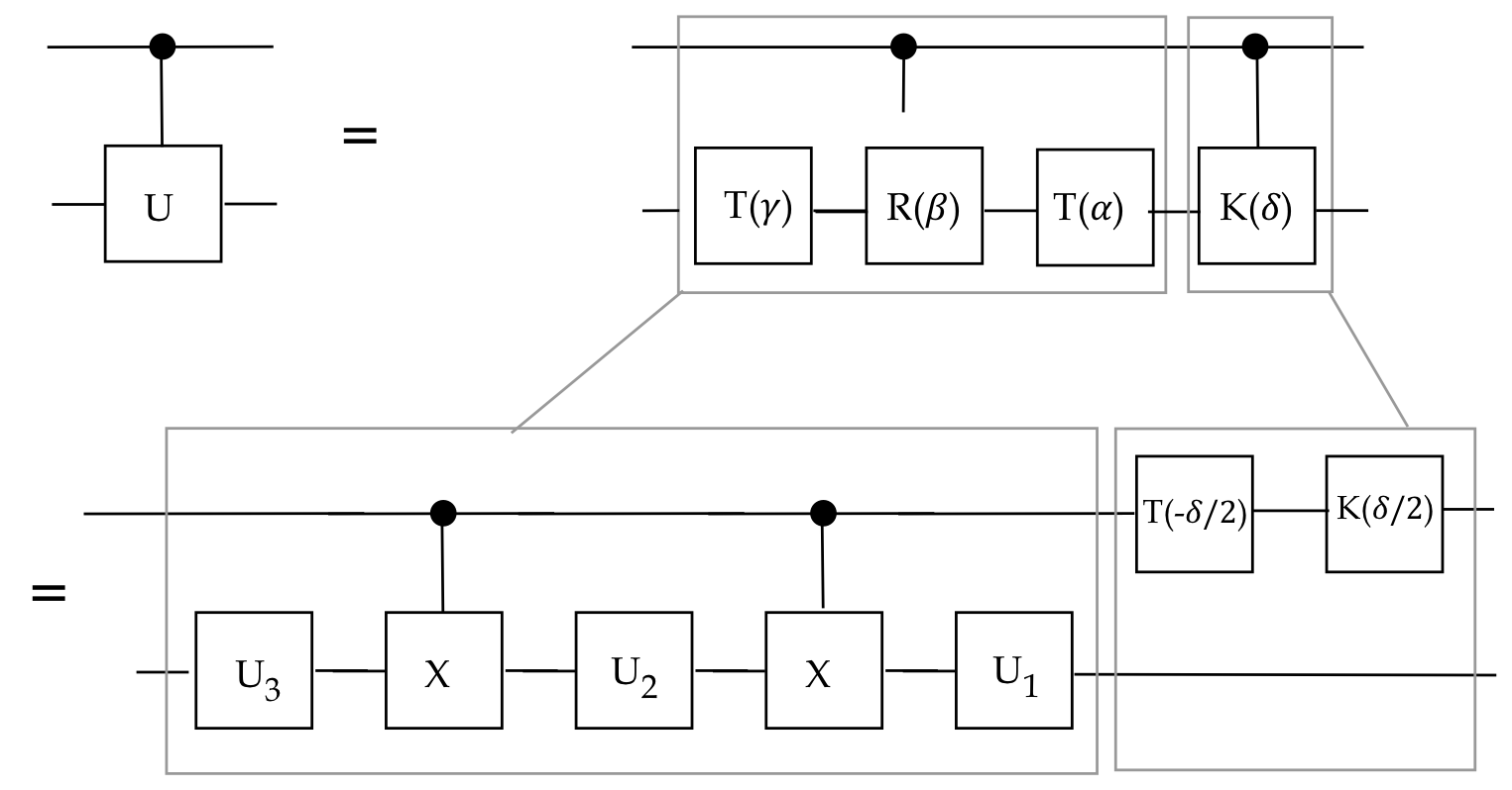
- Thus, we have a way to use basic gates to build any
Controlled-\(U\) gate.
7.3
Controlled-controlled-\(U\)
The previous section showed how a singly-controlled \(U\)
can be expressed in terms of basic gates.
In this section we consider doubly-controlled unitaries.
Because a unitary \(U\) is expressible as \(V^2 = U\) where \(V\) is unitary then the 3-qubit Controlled-controlled-\(U\) can be
computed using only 2-qubit gates:
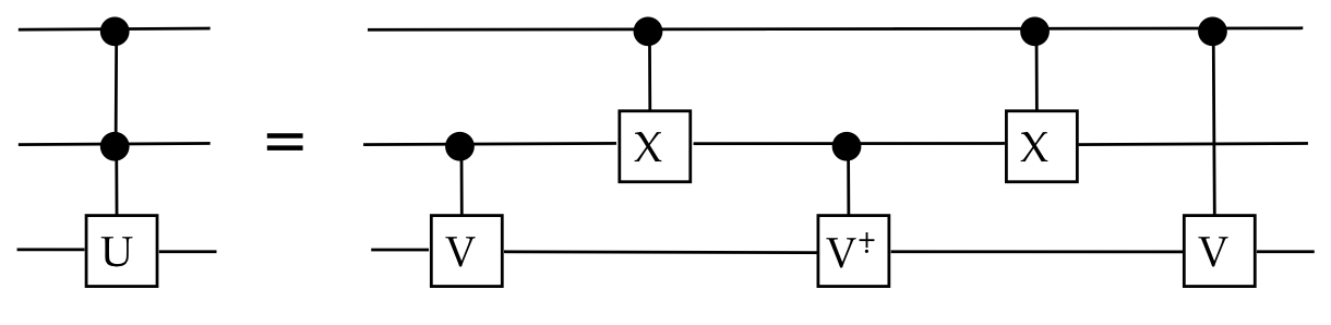
- Here, \(V^2 = U\) and \(V^\dagger = V^{-1}\).
- Let's consider the four cases for the top two qubits:
\(\kt{00}, \kt{01}, \kt{10}, \kt{11}\)
- Case: \(\kt{00}\)
Here, none of the gates will be active, so the 3rd qubit is unchanged.
- Case: \(\kt{01}\)
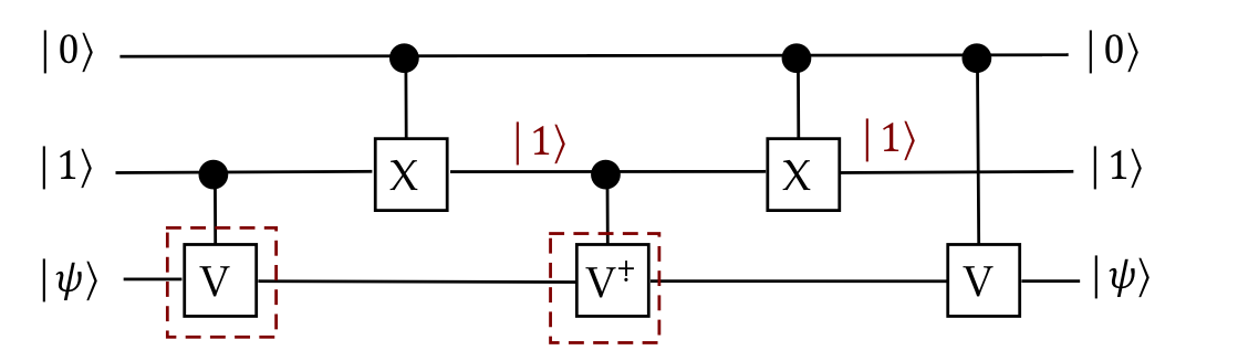
Now the active gates for the 3rd qubit result in
$$
V^\dagger V \ksi \eql \ksi
$$
Thus, no change.
- Case: \(\kt{10}\)
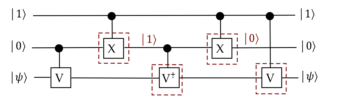
This time, the active gates for the 3rd qubit result in:
$$
V V^\dagger \ksi \eql \ksi
$$
- Case: \(\kt{11}\)
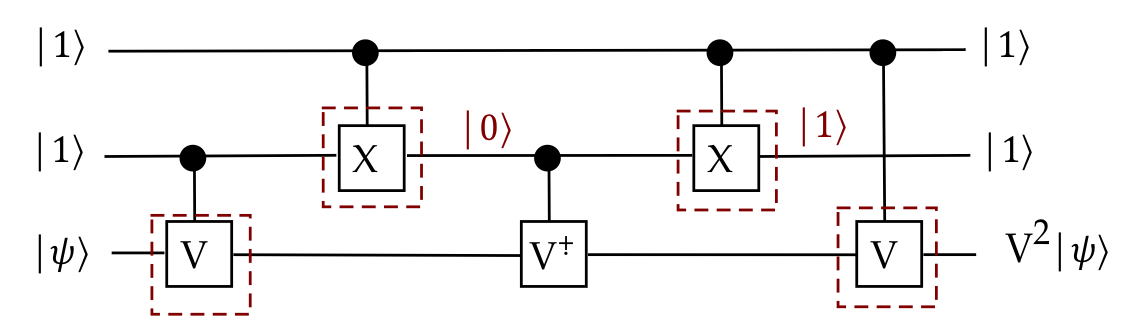
Now we see that
$$
V^2 \ksi \eql U \ksi
$$
as desired.
- Of course, for arbitrary \(U\), it may not be easy
to find \(V\) such that \(V^2=U\):
- For matrices that can be easily exponentiated, we have
seen how to do this.
How can \(V\) be computed?
- The spectral theorem that proves the existence of
orthonormal eigenvectors applies to a broader class of
matrices than Hermitians: the so-called normal matrices:
- \(A\) is normal if \(AA^\dagger = A^\dagger A\).
- Clearly, if \(A\) is Hermitian (\(A=A^\dagger\)), then
\(A\) is normal.
- So are unitaries because, by definition, \(A A^\dagger = I = A^\dagger A\).
- Apply the spectral theorem to write \(U\) as
$$
U \eql S D S^\dagger
$$
where
$$\eqb{
D & \eql & \mbox{ Diagonal matrix with eigenvalues
\(\lambda_i\) diagonal }\\
S & \eql & \mbox{ eigenvectors as columns }
}$$
- Let \(D^{\frac{1}{2}}\) be the matrix with \(\sqrt{\lambda_i}\) on the
diagonal, and zeroes elsewhere. Then,
$$
\parenl{ D^{\frac{1}{2}} }^2 \eql D
$$
- Now define
$$
V \eql S D^{\frac{1}{2}} S^\dagger
$$
- Then
$$
V^2 \eql \parenl{ S D^{\frac{1}{2}} S^\dagger } \parenl{ S D^{\frac{1}{2}} S^\dagger }
\eql
S D^{\frac{1}{2}} (S S^\dagger) D^{\frac{1}{2}} S^\dagger
\eql U
$$
- When computing \(\sqrt{\lambda_i}\), there are two roots,
and thus any choice of roots will result in one particular
solution to \(V^2=U\).
The solution above (to control-control-\(U\)) needed no additional
qubits.
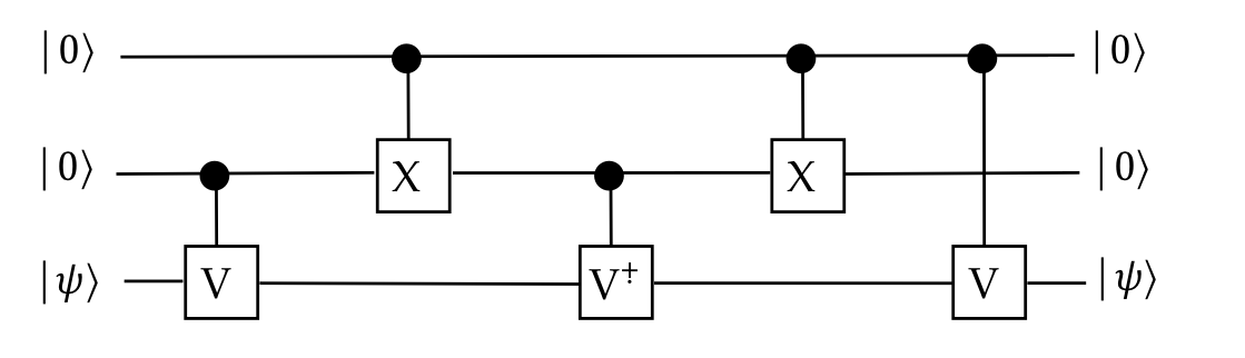
However, with an additional spare qubit, a simpler solution is possible:
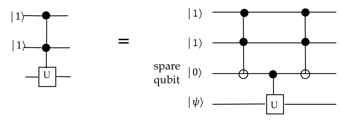
- The solution uses a singly-controlled \(U\).
- It's only when the two control qubits are both \(\kt{1}\)
that the spare becomes \(\kt{1}\).
- And that's when controlled-\(U\) is activated.
7.4
Universality: multiply-controlled \(U\)
The idea above can be extended to any number of control qubits.
Consider the following 4-controlled \(U\):
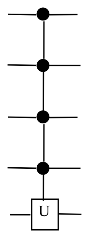
- We can use three additional qubits to achieve the same result
with \(\ccnot\) gates and a doubly-controlled \(U\):
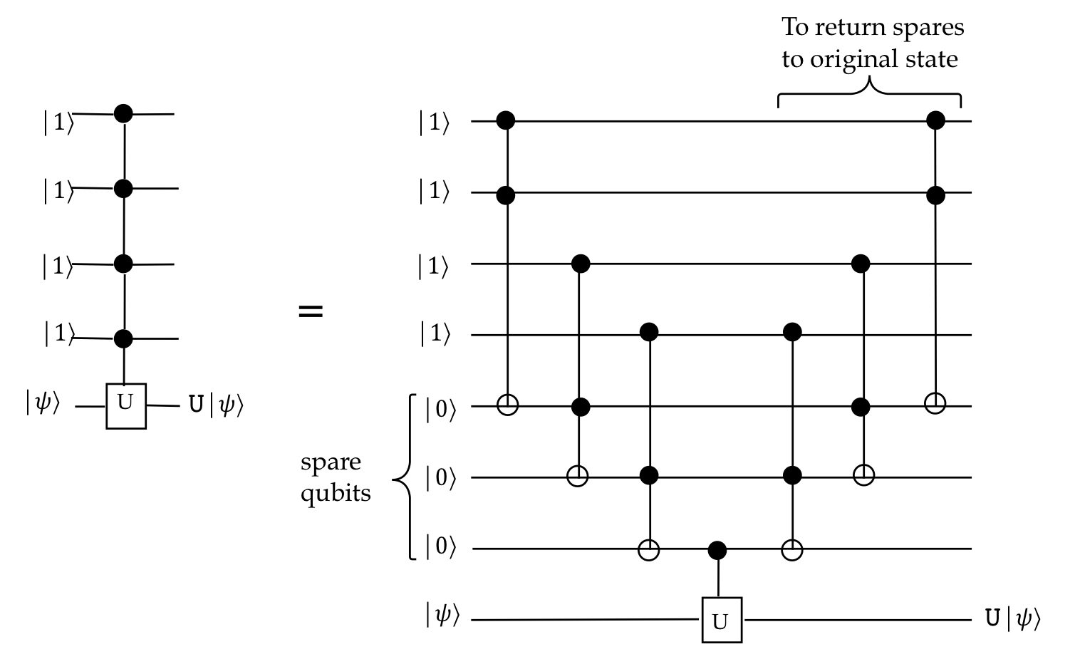
- Clearly, any control-pattern can be accommodated by
using the appropriate \(\ccnot\) gates (filled or unfilled circles).
7.5
Universality: multi-qubit gates
We will now show that an arbitrary n-qubit unitary operation
can be decomposed into multiply-controlled single-qubit operations.
This means that, using the previous sections, any arbitrary
n-qubit unitary can be implemented with controlled-\(U\)'s
and \(\cnot\) gates.
The construction is fairly involved, so let's do this in steps.
Step 1: A two-level unitary affects only two entries in a vector:
- Consider this modification of the 3-qubit identity:
$$
\mat{
1 & 0 & 0 & 0 & 0 & 0 & 0 & 0 \\
0 & {\bf a} & 0 & 0 & 0 & 0 & 0 & 0 \\
0 & 0 & 1 & 0 & 0 & 0 & 0 & 0 \\
0 & 0 & 0 & 1 & 0 & 0 & 0 & 0 \\
0 & 0 & 0 & 0 & 1 & 0 & 0 & 0 \\
0 & 0 & 0 & 0 & 0 & 1 & 0 & 0 \\
0 & 0 & 0 & 0 & 0 & 0 & {\bf d} & 0 \\
0 & 0 & 0 & 0 & 0 & 0 & 0 & 1 \\
}
$$
- We've replaced two of the 1's along the diagonal with complex
numbers \(a\) and \(d\)
- If we want the resulting matrix to be unitary, we will need
to satisfy unit-length (rows and columns), and pairwise
orthogonality amongst rows and columns.
- Accordingly, with minimal additional entries, let's add
$$
\mat{
1 & 0 & 0 & 0 & 0 & 0 & 0 & 0 \\
0 & {\bf a} & 0 & 0 & 0 & 0 & {\bf b} & 0 \\
0 & 0 & 1 & 0 & 0 & 0 & 0 & 0 \\
0 & 0 & 0 & 1 & 0 & 0 & 0 & 0 \\
0 & 0 & 0 & 0 & 1 & 0 & 0 & 0 \\
0 & 0 & 0 & 0 & 0 & 1 & 0 & 0 \\
0 & {\bf c} & 0 & 0 & 0 & 0 & {\bf d} & 0 \\
0 & 0 & 0 & 0 & 0 & 0 & 0 & 1 \\
}
$$
- One can impose the unitarity conditions and obtain
relationships between these numbers, such as:
\(\magsq{a} + \magsq{b} = 1\).
- One possible solution is:
$$
\mat{
1 & 0 & 0 & 0 & 0 & 0 & 0 & 0 \\
0 & {\bf a} & 0 & 0 & 0 & 0 & {\bf c^*} & 0 \\
0 & 0 & 1 & 0 & 0 & 0 & 0 & 0 \\
0 & 0 & 0 & 1 & 0 & 0 & 0 & 0 \\
0 & 0 & 0 & 0 & 1 & 0 & 0 & 0 \\
0 & 0 & 0 & 0 & 0 & 1 & 0 & 0 \\
0 & {\bf c} & 0 & 0 & 0 & 0 & {\bf -a^*} & 0 \\
0 & 0 & 0 & 0 & 0 & 0 & 0 & 1 \\
}
$$
where \(a\) and \(c\) satisfy \(\magsq{a} + \magsq{c} = 1\).
- Next, observe the action of such a matrix on a generic
3-qubit vector:
$$
\mat{
1 & 0 & 0 & 0 & 0 & 0 & 0 & 0 \\
0 & {\bf a} & 0 & 0 & 0 & 0 & {\bf b} & 0 \\
0 & 0 & 1 & 0 & 0 & 0 & 0 & 0 \\
0 & 0 & 0 & 1 & 0 & 0 & 0 & 0 \\
0 & 0 & 0 & 0 & 1 & 0 & 0 & 0 \\
0 & 0 & 0 & 0 & 0 & 1 & 0 & 0 \\
0 & {\bf c} & 0 & 0 & 0 & 0 & {\bf d} & 0 \\
0 & 0 & 0 & 0 & 0 & 0 & 0 & 1 \\
}
\mat{\alpha_0 \\ \alpha_1 \\ \alpha_2 \\ \alpha_3 \\
\alpha_4 \\ \alpha_5 \\ \alpha_6 \\ \alpha_7 }
\eql
\mat{\alpha_0 \\ {\bf a\alpha_1 + b\alpha_6} \\ \alpha_2 \\ \alpha_3 \\
\alpha_4 \\ \alpha_5 \\ {\bf c\alpha_1 + d\alpha_6} \\ \alpha_7 }
$$
Notice: only two entries in the vector are modified.
- In Dirac notation, the result is:
$$
\alpha_0 \kt{000} + {\bf (a\alpha_1 + b\alpha_6) \kt{001}}
\alpha_2\kt{010} + \alpha_3 \kt{011}
+ \alpha_4 \kt{100} + \alpha_5 \kt{101}
+ {\bf (c\alpha_1 + d\alpha_6) \kt{110}} + \alpha_7 \kt{111}
$$
- This corresponds to the two columns for \(\kt{001}\)
and \(\kt{110}\).
- Thus, another way of saying "two entries are modified" is:
the coefficients of two standard-basis vectors are modified.
- In general, for n-qubits:
- The resulting \(2^n \times 2^n\)
matrix will have two columns in which the four numbers lie.
- These columns will correspond to the two standard-basis
vectors that get modified.
- We will call such a matrix a two-level unitary matrix.
- Note: the adjoint of a two-level unitary is a
two-level unitary.
$$
\mat{
1 & 0 & 0 & 0 & 0 & 0 & 0 & 0 \\
0 & {\bf a} & 0 & 0 & 0 & 0 & {\bf c^*} & 0 \\
0 & 0 & 1 & 0 & 0 & 0 & 0 & 0 \\
0 & 0 & 0 & 1 & 0 & 0 & 0 & 0 \\
0 & 0 & 0 & 0 & 1 & 0 & 0 & 0 \\
0 & 0 & 0 & 0 & 0 & 1 & 0 & 0 \\
0 & {\bf c} & 0 & 0 & 0 & 0 & {\bf -a^*} & 0 \\
0 & 0 & 0 & 0 & 0 & 0 & 0 & 1 \\
}^\dagger
\eql
\mat{
1 & 0 & 0 & 0 & 0 & 0 & 0 & 0 \\
0 & {\bf a^*} & 0 & 0 & 0 & 0 & {\bf c^*} & 0 \\
0 & 0 & 1 & 0 & 0 & 0 & 0 & 0 \\
0 & 0 & 0 & 1 & 0 & 0 & 0 & 0 \\
0 & 0 & 0 & 0 & 1 & 0 & 0 & 0 \\
0 & 0 & 0 & 0 & 0 & 1 & 0 & 0 \\
0 & {\bf c} & 0 & 0 & 0 & 0 & {\bf -a} & 0 \\
0 & 0 & 0 & 0 & 0 & 0 & 0 & 1 \\
}
$$
Step 2: Any unitary can be expressed as a
product of two-level unitaries:
- We'll use a 2-qubit example to explain how.
- Consider
$$
U \eql
\mat{ u_{00} & u_{01} & u_{02} & u_{03} \\
u_{10} & u_{11} & u_{12} & u_{13} \\
u_{20} & u_{21} & u_{22} & u_{23} \\
u_{30} & u_{31} & u_{32} & u_{33} \\
}
$$
- We'll now apply a series of matrix multiplications to
convert \(U\) into the identity.
- Recall from row-reduced matrices in solving equations: we
want to make the entries below \(u_{00}\) all 0.
- We want to multiply \(U\) by a matrix \(U_1\) to make
the entry below \(u_{00}\) zero:
$$
U_1 U \eql
\mat{ u_{00} & u_{01} & u_{02} & u_{03} \\
{\bf 0} & u_{11} & u_{12} & u_{13} \\
u_{20} & u_{21} & u_{22} & u_{23} \\
u_{30} & u_{31} & u_{32} & u_{33} \\
}
$$
- Clearly, the second row of \(U_1\) produces that number,
and so
$$
U_1 \eql
\mat{1 & 0 & 0 & 0\\
u_{10} & -u_{00} & 0 & 0\\
0 & 0 & 1 & 0\\
0 & 0 & 0 & 1
}
$$
achieves the result.
- But \(U_1\) is not unitary.
- To fix this, we adjust the "two-level" entries as we did
with two-level unitaries so that
$$
U_1 \eql
\mat{\frac{u_{00}^*}{r_1} & \frac{u_{10}^*}{r_1} & 0 & 0\\
\frac{u_{10}}{r_1} & -\frac{u_{00}}{r_1} & 0 & 0\\
0 & 0 & 1 & 0\\
0 & 0 & 0 & 1
}
$$
where \(\magsq{u_{00}} + \magsq{u_{10}} = r_1^2\)
is both unitary and two-level (which will play a later role).
- Multiplication by \(U_1\) will produce some result we'll call \(B\):
$$
U_1 U
\eql
\mat{\frac{u_{00}^*}{r_1} & \frac{u_{10}^*}{r_1} & 0 & 0\\
\frac{u_{10}}{r_1} & -\frac{u_{00}}{r_1} & 0 & 0\\
0 & 0 & 1 & 0\\
0 & 0 & 0 & 1
}
\mat{ u_{00} & u_{01} & u_{02} & u_{03} \\
u_{10} & u_{11} & u_{12} & u_{13} \\
u_{20} & u_{21} & u_{22} & u_{23} \\
u_{30} & u_{31} & u_{32} & u_{33} \\
}
\eql
\mat{ \alpha & b_{01} & b_{02} & b_{03} \\
0 & b_{11} & b_{12} & b_{13} \\
b_{20} & b_{21} & b_{22} & b_{23} \\
b_{30} & b_{31} & b_{32} & b_{33} \\
}
\eql B
$$
Note that the top left number is some \(\alpha\).
- Proceeding, we can zero the entry \(b_{20}\) through
multiplication by
$$
U_2 \eql
\mat{ \frac{b_{00}^*}{r_2} & 0 & \frac{b_{20}^*}{r_2} & 0 \\
0 & 1 & 0 & 0 \\
\frac{b_{20}}{r_2} & 0 & -\frac{b_{00}}{r_2} & 0 \\
0 & 0 & 0 & 1 \\
}
$$
so that
$$
U_2 B \eql U_2 U_1 U
\eql
\mat{ \beta & c_{01} & c_{02} & c_{03} \\
0 & c_{11} & c_{12} & c_{13} \\
{\bf 0} & c_{21} & c_{22} & c_{23} \\
c_{30} & c_{31} & c_{32} & c_{33} \\
}
\eql C
$$
where we're calling the result \(C\).
- Finally, one more multiplication by a two-level matrix
will produce the final zero in the first column:
$$
D \eql U_3 C \eql U_3 U_2 U_1 U
\eql
\mat{ 1 & d_{01} & d_{02} & d_{03} \\
0 & d_{11} & d_{12} & d_{13} \\
0 & d_{21} & d_{22} & d_{23} \\
{\bf 0} & d_{31} & d_{32} & d_{33} \\
}
$$
- This time, the top left number must be 1. Why?
- We have already shown that the multiplying
matrices \(U_i\) are unitary.
- This makes \(D\) unitary, since the product of unitaries is unitary.
- All the other numbers in the first column are 0.
- Because a column must have unit length, that makes the top
left number 1.
- Next, a pleasant windfall:
- Since \(D\) is unitary, the first row has length 1.
- This necessarily means the entries other than the top left
are all 0:
$$
D
\eql
\mat{ 1 & {\bf 0} & {\bf 0} & {\bf 0} \\
0 & d_{11} & d_{12} & d_{13} \\
0 & d_{21} & d_{22} & d_{23} \\
0 & d_{31} & d_{32} & d_{33} \\
}
$$
- Thus, no additional operations are needed to make the first
row the same as the identity's first row.
- Once the first column and row are the same as in \(I\),
further reductions can be applied to make the second column and row
the same as in I.
- Once the second row is done, we do the third, and so on.
- We'll describe the entire sequence of unitary multiplications
as
$$
U_k U_{k-1} \ldots U_1 U \eql I
$$
- Which means
$$
U \eql U_1^\dagger \ldots U_l^\dagger
$$
- Each \(U_i^\dagger\) is a two-level unitary.
- Thus, we have shown: any unitary \(U\) can be
expressed as a product of two-level unitaries.
Step 3: A circuit for a two-level unitary that
uses only controlled single-qubit gates
- The goal is to show how one of the \(U_i^\dagger\)'s
can be implemented with controlled 1-qubit gates.
- If this can be done, each multiply-controlled 1-qubit
gate can itself be decomposed into 1-qubit gates and \(\cnot\) gates.
- We'll show how this works using an example.
- Consider the unitary
$$
U_i^\dagger
\eql
\mat{
1 & 0 & 0 & 0 & 0 & 0 & 0 & 0 \\
0 & {\bf a} & 0 & 0 & 0 & 0 & {\bf b} & 0 \\
0 & 0 & 1 & 0 & 0 & 0 & 0 & 0 \\
0 & 0 & 0 & 1 & 0 & 0 & 0 & 0 \\
0 & 0 & 0 & 0 & 1 & 0 & 0 & 0 \\
0 & 0 & 0 & 0 & 0 & 1 & 0 & 0 \\
0 & {\bf c} & 0 & 0 & 0 & 0 & {\bf d} & 0 \\
0 & 0 & 0 & 0 & 0 & 0 & 0 & 1 \\
}
$$
where \(a,b,c,d\) are complex numbers.
- This matrix changes only two coefficients in
a generic vector:
$$
U_i^\dagger
\eql
\mat{
1 & 0 & 0 & 0 & 0 & 0 & 0 & 0 \\
0 & {\bf a} & 0 & 0 & 0 & 0 & {\bf b} & 0 \\
0 & 0 & 1 & 0 & 0 & 0 & 0 & 0 \\
0 & 0 & 0 & 1 & 0 & 0 & 0 & 0 \\
0 & 0 & 0 & 0 & 1 & 0 & 0 & 0 \\
0 & 0 & 0 & 0 & 0 & 1 & 0 & 0 \\
0 & {\bf c} & 0 & 0 & 0 & 0 & {\bf d} & 0 \\
0 & 0 & 0 & 0 & 0 & 0 & 0 & 1 \\
}
\mat{\alpha_0 \\ \alpha_1 \\ \alpha_2 \\ \alpha_3 \\
\alpha_4 \\ \alpha_5 \\ \alpha_6 \\ \alpha_7 }
\eql
\mat{\alpha_0 \\ {\bf a\alpha_1 + b\alpha_6} \\ \alpha_2 \\ \alpha_3 \\
\alpha_4 \\ \alpha_5 \\ {\bf c\alpha_1 + d\alpha_6} \\ \alpha_7 }
$$
- Thus, we need a circuit to accomplish:
$$\eqb{
U_i^\dagger \alpha_0\kt{000} & \eql & \alpha_0\kt{000} \\
U_i^\dagger \alpha_1\kt{001} & \eql & {\bf (a\alpha_1 + b\alpha_6) \kt{001}} \\
U_i^\dagger \alpha_2\kt{010} & \eql & \alpha_2\kt{010} \\
U_i^\dagger \alpha_3\kt{011} & \eql & \alpha_3\kt{011} \\
U_i^\dagger \alpha_4\kt{100} & \eql & \alpha_4\kt{100} \\
U_i^\dagger \alpha_5\kt{101} & \eql & \alpha_5\kt{101} \\
U_i^\dagger \alpha_6\kt{110} & \eql & {\bf (c\alpha_1 + d\alpha_6) \kt{110}}\\
U_i^\dagger \alpha_7\kt{111} & \eql & \alpha_7\kt{111} \\
}$$
- So, somehow, the control qubits must be set up so that
\(\kt{001}\) and \(\kt{110}\) activate gates to transform these
two, while the other states stay the same.
- We will rewrite the two \(\alpha_i\) coefficients as
$$\eqb{
U_i^\dagger p\kt{001} & \eql & {\bf (ap + bq) \kt{001}} \\
U_i^\dagger q\kt{110} & \eql & {\bf (cp + dq) \kt{110}}\\
}$$
- Suppose that, instead of \(\kt{001}\) and \(\kt{110}\),
we had states \(\kt{010}\) and \(\kt{110}\):
- The binary representations differ by just one bit.
- Terminology: they are grey-code adjacent.
- Next, let
$$
V \eql \mat{a & b\\ c & d}
$$
and observe that
$$\eqb{
V\kt{0} & \eql & \mat{a & b\\ c & d} \mat{1\\ 0}
& \eql & \mat{a\\ c} & \eql & a\kt{0} + c\kt{1} \\
V\kt{1} & \eql & \mat{a & b\\ c & d} \mat{0\\ 1}
& \eql & \mat{b\\ d} & \eql & b\kt{0} + d\kt{1} \\
}$$
- Now consider the circuit
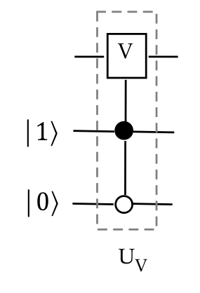
- Here, when the 2nd and 3rd qubits are in \(\kt{10}\), the
\(V\) gate is applied.
- Thus, the only two 3-qubit vectors that will activate \(V\)
are the adjacent states \(\kt{010}\) and \(\kt{110}\).
- Suppose the 3-qubit unitary \(U_V\) describes the controlled
gate above.
- Then, for any linear combination of \(\kt{010}\) and \(\kt{110}\)
$$\eqb{
U_V (p\kt{010} + q\kt{110})
& \eql &
pV\kt{0}\kt{10} + qV\kt{1}\kt{10} \\
& \eql &
p (a\kt{0}+c\kt{1}) \kt{10} + q (b\kt{0} + d\kt{1}) \kt{10} \\
& \eql &
(ap + bq)\kt{0}\kt{10} + (bp+dq) \kt{1} \kt{10} \\
& \eql &
(ap + bq)\kt{010} + (bp+dq) \kt{110} \\
}$$
- This suggests that we can make the desired two-level-unitary
action work for adjacent vectors.
- To make it work for our original pair \(\kt{001}\) and \(\kt{110}\),
we form a "word ladder" to go from \(\kt{001}\) to \(\kt{010}\):
$$
001 \; \rightarrow \; 000 \; \rightarrow \; 010
$$
which is adjacent to \(\kt{110}\).
- We already know how to do vector conversions where two
successive vectors different by a bit in the binary
representation.
- Let's draw the circuit for this example:
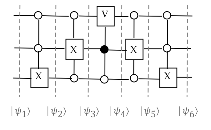
Then for
$$
\kt{\psi_1} \eql p\kt{001} + q\kt{110}
$$
we get
$$\eqb{
\kt{\psi_2} & \eql & p\kt{000} + q\kt{110} \\
\kt{\psi_3} & \eql & p\kt{010} + q\kt{110} \\
\kt{\psi_4} & \eql & (ap + bq)\kt{010} + (bp+dq)\kt{110} \\
\kt{\psi_5} & \eql & (ap + bq)\kt{000} + (bp+dq)\kt{110} \\
\kt{\psi_6} & \eql & (ap + bq)\kt{001} + (bp+dq)\kt{110} \\
}$$
- The latter two return the transformed state \(\kt{010}\)
back to the original \(\kt{001}\).
- The same circuit does nothing to the other standard-basis
vectors.
- Each of the above multiply-controlled 1-qubit operation can
be decomposed into 1-qubit standard gates and \(\cnot\) gates.
- So, finally, we have a circuit for an arbitrary two-level matrix.
- Let's state this as a theorem:
Theorem 7.1:
An arbitrary n-qubit unitary can be
constructed out of 1-qubit standard gates and \(\cnot\) gates.
How many gates?
- Unfortunately, the decomposition we've described needs an
exponential number of gates.
- Consider the breakdown into two-level unitaries:
- The starting point is a \(N\times N = 2^n \times 2^n\) matrix.
- It takes \(N-1\) steps to create zeroes in the first column
(and row).
- Then, \(N-2\) for the second column, and so on.
- Thus, overall: \(N-1 + N-2 + \ldots + 1 = N(N-1)/2\)
two-level unitaries.
- This is approximately of the order of \(N^2 = 2^{2n}\)
- This is already exponential (in the number of qubits).
- The staging of each two-level unitary is linear, because
at most 1-bit "word ladder" changes are needed for any two-level unitary.
- Thus, while theoretically interesting, it is not a practical approach.
Theoretical results about approximation:
- One might ask: is it possible to approximate a unitary with
circuit that has a polynomial number of gates?
- Unfortunately, the answer is no.
- For any given set of gates, one can construct qubit
states that will need an exponential number of gates
to construct from the all-0 state.
- Of course, this says little about the types of unitaries
that tend to appear in well-known algorithms.
- A related approximation result: the famous Solovay-Kitaev theorem.
- This is about 1-qubit unitaries.
- Recall: we showed how to use K, R, T gates to construct any
unitary.
- However, the parameters of these gates were determined by
solving equations.
- What if your hardware had only a fixed set of gates with
fixed parameters?
- The S-K theorem shows that, nonetheless, it's possibly to
efficiently approximate any 1-qubit unitary with a polynomial
number of gates from a fixed set.