Module objectives
Quantum chemistry is considered a viable and useful first goal
for quantum computing.
The purpose of this module is to understand the "how" (algorithms)
of the central computational task: finding the ground state energy
of a molecule.
Note:
- Alert regarding possible notational confusion:
- We've used \(H\) for the Hadamard unitary operator in
circuits.
- However, \(H\) is also used for the Hamiltonian operator.
- In this module, \(H\) is most often the Hamiltonian.
- We'll point out specifically when \(H\) is the Hadamard.
- Caveat emptor: my knowledge of Chemistry is modest; the material
below is synthesized from the references at the end.
12.1
What is quantum computational chemistry and why is it important?
Let's start with some grand-challenge problems in chemistry:
- Better molecules for existing processes:
- Example: producing fertilizer takes up 2% of worldwide human energy
consumption.
- An improved (Bosch-Haber) catalyst could signifcantly reduce
this cost.
- New drugs:
- It costs billions to design, test and deploy a new drug.
- Computation can help determine more viable candidates.
How does computation help?
- Let's take a closer look at the hit-or-miss
modern drug design process:
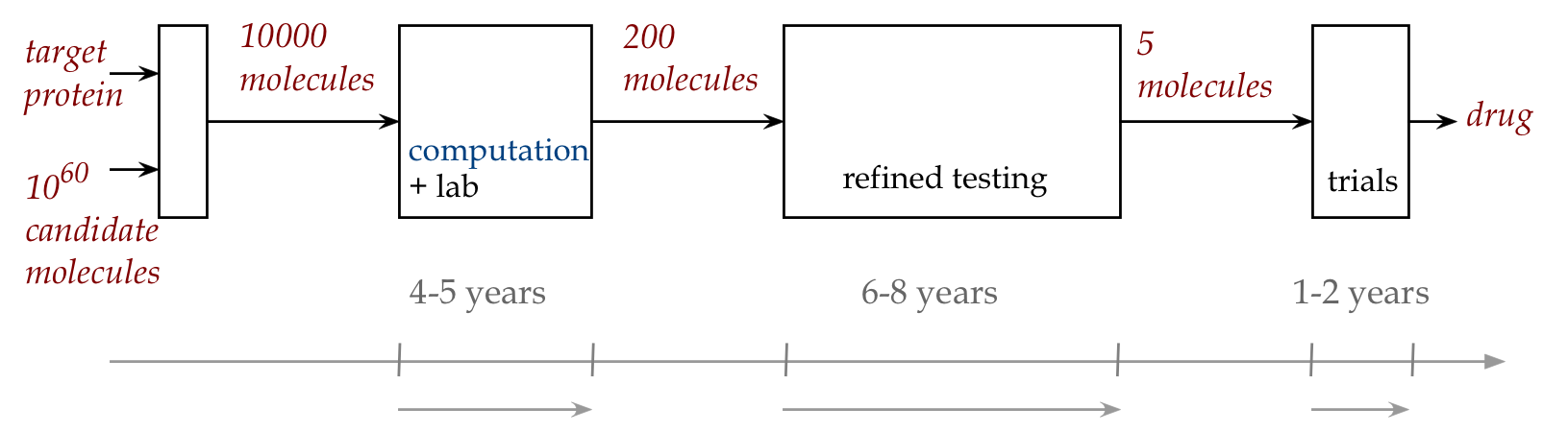
- Drug design is complicated because of physiological
constraints on chemistry
\(\rhd\)
Examples: oral intake, solubility, narrow temperature range (\(98.6^{\circ} F\)).
- Accurate simulation of chemistry can reduce lab time/costs,
and reduce the number of strong-candidate molecules.
What is being computed?
- Typically, a drug is designed to bind to some target
protein (often to disable it).
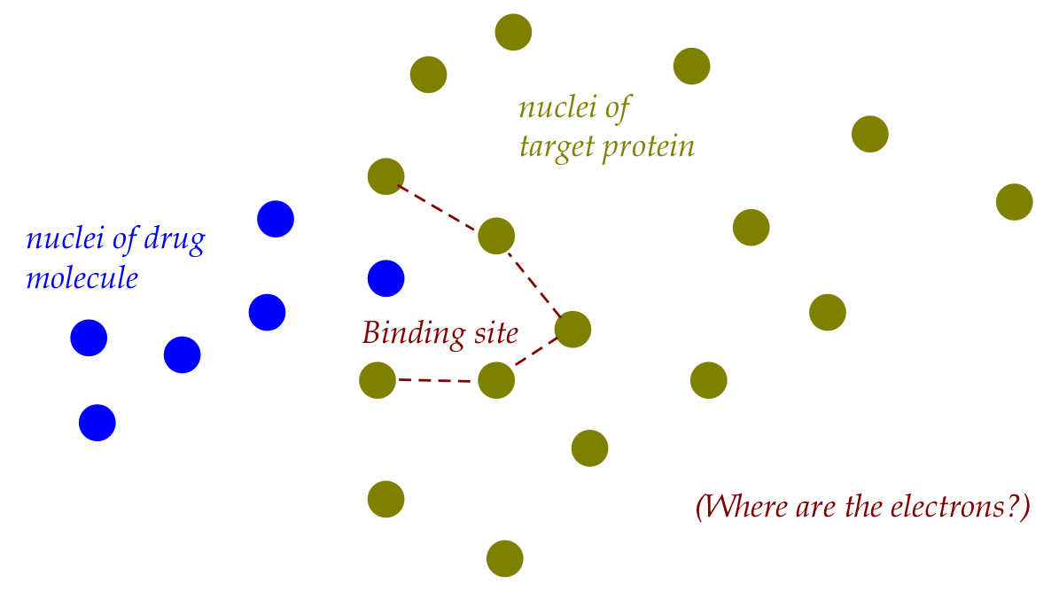
Note:
- The diagram shows tentative positions of nuclei.
\(\rhd\)
A common approximation is to assume fixed locations for nuclei.
- The goal is to figure out where the electrons end up in the
lowest-energy state.
- One type of desired analysis:
- Start with the most stable configuration for the
"unbound" drug
\(\rhd\) the ground state
(lowest energy)
- Then, discover the highest (activation) energy that must
surpassed in order for the reaction proceed.
- This can be done with various nuclei configurations to
explore what's possible.
- Another type of analysis:
- See if the drug can bind in the target "pocket" of the protein.
- To do so, examine various nuclei coordinates and compute the
minimum energy.
- There are two classical-computing approaches:
- Use classical mechanics (forces etc) to model electron interactions.
- Use quantum mechanics, but compute classically.
- The main goal, computationally: solve the electronic structure
- Describe the wave functions of the electrons.
- The classical-mechanics approach (molecular dynamics) is
only approximate:
- After all, electrons (and nuclei) are complicated quantum objects.
- They don't have fixed position, for example.
- The quantum-mechanics approach is accurate, but hard to
compute with a classical computer.
What is the quantum-mechanics approach?
- It all boils down to solving an eigenvalue problem:
$$
H \kt{\psi_0} \eql \lambda_0 \kt{\psi_0}
$$
where
$$\eqb{
\kt{\psi_0} & \eql & \mbox{the ground state} \\
\lambda_0 & \eql & \mbox{the energy of the ground state} \\
H & \eql & \mbox{the Hamiltonian for the system}
}$$
Note: once approximated, \(H\) becomes a Hermitian matrix.
- Let's take a closer look.
- First, let's examine what "state" means:
- We've seen: a group of qubits is in a joint state (a
big vector) at any time.
- Similarly, a group of quantum objects (electrons etc)
is in a joint state at any time.
- That state has parameters: location variables, time, etc.
- Thus, \(\kt{\psi(x,t)}\) represents the state of a
one-dimensional object, parametrized by variables for location and
time.
- And,
$$
\kt{\psi({\bf r},t)}
$$
represents the time-varying state of a 3D quantum object like an electron.
- Here,
$$
{\bf r} \eql (x,y,z)
$$
a 3D coordinate (location) vector.
- Recall the Schrodinger equation:
$$
i\hbar \frac{\partial }{\partial t} \kt{\psi({\bf r},t)} \eql H(t) \kt{\psi({\bf r},t)}
$$
Here, \(H(t)\) is an operator (potentially itself time-varying)
called the quantum Hamiltonian operator
constructed in a particular way:
- Classical quantities like position \(x\) and momentum \(p\)
are replaced by corresponding quantum operators to form \(H\).
- Typically, one assumes \(H(t) = H\) (not varying with time):
$$
i\hbar \frac{\partial}{\partial t} \kt{\psi({\bf r},t)} \eql H \kt{\psi({\bf r},t)}
$$
- It turns out that solutions to the equation can be expressed
in terms of the eigenbasis of \(H\), i.e., basis states
\(\kt{\psi_0}, \kt{\psi_1}, \ldots \) such that
$$
H \kt{\psi_i} \eql \lambda_i \kt{\psi_i}
$$
- It turns out that
$$
\lambda_i \eql \mbox{the energy associated with state } \kt{\psi_i}
$$
- The numbering is such that
$$
\kt{\psi_0} \eql \mbox{state with the lowest energy}
$$
This is the state we want to identify, along with its eigenvalue:
$$
H \kt{\psi_0} \eql \lambda_0 \kt{\psi_0}
$$
- For a computational approach, the problem needs to be
discretized in some way.
\(\rhd\)
Then, \(H\) becomes a matrix.
- The computational problem, then, is:
- Calculate (or estimate) \(\kt{\psi_0}\).
- Solve for \(\lambda_0\) in
\(
H \kt{\psi_0} \eql \lambda_0 \kt{\psi_0}
\)
- The main challenge: \(H\) can be quite large.
- Example: so-called (simplified) electronic Hamiltonian
with orbital-occupancy:
- \(n_e\) possible electron orbitals, \(k_e\) electrons.
- How many possible assignments of electrons to orbitals?
- Answer:
\(
\nchoose{n_e}{k_e}
\)
- Example: \(H_2 O\) (simplified) \(n_e=14, k_e=10\)
\(\rhd\) \(\approx 1000\) configurations
- Example: \(H_2 O\) (refined) \(n_e=116, k_e=10\)
\(\rhd\) \(\approx 10^{23}\) configurations
- Note: \(10^{23} \approx 2^{77}\)
\(\rhd\) \(2^{77}\) basis states
\(\rhd\)
matrix size (for any operator) is \(2^{77} \times 2^{77}\).
- Can a quantum computer help?
12.2
Two quantum computing approaches to solving \( H \kt{\psi_0} \eql \lambda_0 \kt{\psi_0}\)
We'll provide a high-level overview, with details to follow in
later sections.
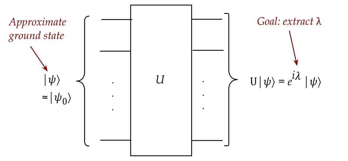
The first approach: constructing and applying a unitary
- \(H\), the Hamiltonian, is a Hermitian matrix.
- Then, \(U = e^{iH}\) is unitary and
$$\eqb{
U \kt{\psi_0} & \eql & e^{iH} \kt{\psi_0}\\
& \eql & \left( 1 + iH + \frac{i^2H^2}{2!} + \ldots \right)
\kt{\psi_0} \\
& \eql & \kt{\psi_0} + iH \kt{\psi_0} +
\frac{i^2H^2}{2!} \kt{\psi_0} + \ldots \\
& \eql & \kt{\psi_0} + i\lambda_0 \kt{\psi_0}
+ i^2\lambda_0^2 \kt{\psi_0} + \ldots \\
& \eql & \left(1 + i\lambda_0 + i^2\lambda_0^2 + \ldots \right)
\kt{\psi_0}\\
& \eql & e^{i\lambda_0} \kt{\psi_0}
}$$
- Make a good guess for \(\kt{\psi_0}\):
$$
\ksi \approx \kt{\psi_0}
$$
- Apply the unitary \(U\) (via a circuit) to \(\kt{\psi}\), to
produce the state \(e^{i\lambda} \kt{\psi}\).
- Somehow (and this is not obvious), extract the constant \(\lambda\).
- Note: mere measurement will result in losing the (global) phase
\(e^{i\lambda}\).
- Then, hopefully, \(\lambda \approx \lambda_0\)
- Two algorithms: Kitaev's algorithm, Abrams-Lloyd algorithm
- Repeat the process with a different (hopefully better) guess
for \(\kt{\psi_0}\).
Second approach: estimate \(\lambda_0\) directly from hardware
- To see how this works, let's recall a few features of measurement.
- Suppose \(\psi_0, \psi_1,\ldots,\psi_{N-1}\) is a measurement basis.
- The projectors are \(P_i = \otr{\psi_i}{\psi_i}\).
- When a measurement occurs, the outcome will be
- One of the basis vectors \(\psi_i\).
- An associated physical quantity \(\lambda_i\) (such as energy).
- The probability of observing the i-th such outcome when
measuring state \(\ksi\) is
\(\swich{\psi}{P_i}{\psi}\).
- The matrix
$$
A \eql \sum_i \lambda_i \otr{\psi_i}{\psi_i}
$$
is a Hermitian with eigenvectors
\(\psi_0, \psi_1,\ldots,\psi_{N-1}\)
and eigenvalues \(\lambda_0,\lambda_1,\ldots,\lambda_{N-1}\).
- Suppose we repeat the measurement many
times and happen to obtain, say,
$$
\lambda_3, \lambda_0, \lambda_2, \lambda_2, \lambda_5, \ldots
$$
- The average eigenvalue obtained is
$$
\frac{\lambda_3 + \lambda_0 + \lambda_2 + \lambda_2 +
\lambda_5 + \ldots}{
\mbox{# measurements}
}
$$
- This number estimates the expected-eigenvalue.
- The expected eigenvalue can be written as:
$$\eqb{
\exval{\mbox{eigenvalue}} & \eql &
\sum_i \lambda_i \prob{\mbox{i-th value occurs}} \\
& \eql &
\sum_i \lambda_i \swich{\psi}{P_i}{\psi} \\
& \eql &
\swich{\psi}{\sum_i \lambda_i P_i}{\psi} \\
& \eql &
\swich{\psi}{A}{\psi} \\
}$$
- Thus, the term \(\swich{\psi}{A}{\psi}\) is
short-hand for expected-eigenvalue for Hermitian \(A\).
- Let's now ask: what would we get for
\(\swich{\psi}{A}{\psi}\) if \(\ksi = \kt{\psi_0}\)?
- That is, we have the system in state \(\kt{\psi_0}\).
- Since
$$
A \eql \sum_i \lambda_i \otr{\psi_i}{\psi_i}
$$
we get
$$\eqb{
\swich{\psi_0}{A}{\psi_0} & \eql &
\swich{\psi_0}{\sum_i \lambda_i \otr{\psi_i}{\psi_i} }{\psi_0} \\
& \eql & \inr{\psi_0}{ \lambda_0 \psi_0}\\
& \eql & \lambda_0
}$$
As one would expect.
- Since we can only guess \(\kt{\psi_0}\), one hopes that
\(\ksi \approx \kt{\psi_0}\).
- In this case,
$$
\swich{\psi}{A}{\psi} \approx \lambda_0
$$
which gives us our approximate estimate of \(\lambda_0\).
- Thus, we'll make repeated measurements so that
$$
\mbox{average of \(\lambda\)'s measured} \; \approx \; \lambda_0
$$
For each measurement, we'll have to reset the state to \(\ksi \approx \kt{\psi_0}\).
- This is the foundation of the
Variational Quantum Eigensolver (VQE) algorithm.
In the following, we'll describe the three algorithms, along with
the background needed:
- Kitaev's algorithm:
- Simplify the Hamiltonian \(H\).
- Construct the corresponding unitary \(U\) so that
$$
U \kt{\psi_0} \eql e^{i\lambda_0} \kt{\psi_0}
$$
- Force \(\lambda_0\) into different coefficients.
- Estimate any one coefficient and then solve for \(\lambda_0\).
- Abrams-Lloyd algorithm:
- Simplify the Hamiltonian \(H\).
- Construct the corresponding unitary \(H\) so that
$$
U \kt{\psi_0} \eql e^{i\lambda_0} \kt{\psi_0}
$$
- Force the digits of \(\lambda_0\) into coefficients of
different qubits.
- Use the inverse QFT to those qubits to recover \(\lambda_0\).
- VQE algorithm:
- Simplify the Hamiltonian \(H\) into Pauli-string operators.
- Guess \(\kt{\psi} \approx \kt{\psi_0}\)
- Perform Pauli measurements.
- Estimate \(\lambda_0\) through observed eigenvalues through averaging.
- Improve the guess \(\ksi\) and repeat.
- All three algorithms start by simplifying (and
approximating) the given Hamiltonian of interest.
12.3
Simplifying Hamiltonians
The simplification and approximation of Hamiltonian matrices is a rich
sub-field by itself, spanning nearly 100 years, too much to summarize here.
We will focus on two major ideas of relevance to quantum
computing.
The first: mapping discretized molecular states to qubit states
- To use the standard circuit model, we have to be able to work
with standard-basis vectors.
- Suppose \(k_e\) electrons are to be placed in \(n_e\) possible
locations (or parameter settings).
- We'll use \(n\) qubits, with \(N = 2^n\).
- Suppose we use the i-th qubit to represent
$$\eqb{
\kt{0} & \eql & \mbox{ no electron present} \\
\kt{1} & \eql & \mbox{ electron present} \\
}$$
- Then, the qubit states \(\kt{0},\kt{1},\ldots,\kt{N-1}\)
are used to represent all possible electron configurations
(including some that can't occur).
- Example: 2 electrons in 3 possible orbitals:
$$\eqb{
\kt{000} & \; & \mbox{no electrons} \\
\kt{001} & \; & \mbox{1 electron} \\
\kt{010} & \; & \mbox{1 electron} \\
\kt{011} & \; & \mbox{2 electrons: valid configuration} \\
\kt{100} & \; & \mbox{1 electron} \\
\kt{101} & \; & \mbox{2 electrons: valid configuration} \\
\kt{110} & \; & \mbox{2 electrons: valid configuration} \\
\kt{111} & \; & \mbox{3 electrons} \\
}$$
This is an example of a simplified direct-occupancy mapping.
- A smarter mapping can reduce the number of qubits to 2
qubits, recognizing that only 3 states above are needed.
(But that complicates the Hamiltonian simplification.)
- In practice, mappings need to satisfy physical constraints
such as "fermionic symmetry" (a property having to do with signs).
The second: writing a Hamiltonian in terms of Pauli-string operators
- Recall our goal: we're given a Hamiltonian as a (often big)
matrix \(H\) and we want the smallest eigenvalue and its
corresponding eigenvector:
$$
H \kt{\psi_0} \eql \lambda_0 \kt{\psi_0}
$$
- Often, we will use a guess \(\ksi \approx \kt{\psi_0}\).
- The guess is constructed with a classical algorithm.
- Then, use \(\ksi\) to solve for \(\lambda_0\).
- To get a feel for how \(H\) can be simplified, we will look
at one approach: writing \(H\) in terms of Pauli-string operators.
- Recall the Pauli matrices \(I, X, Y, Z\):
$$\eqb{
I & \eql & \otr{0}{0} + \otr{1}{1} & \eql & \mat{1 & 0\\0 & 1} \\
X & \eql & \otr{0}{1} + \otr{1}{0} & \eql & \mat{0 & 1\\1 & 0} \\
Y & \eql & -i\otr{0}{1} + i\otr{1}{0} & \eql & \mat{0 & -i\\i & 0} \\
Z & \eql & \otr{0}{0} - \otr{1}{1} & \eql & \mat{1 & 0\\0 & -1} \\
}$$
- Of these, we'll focus on \(X, Y, Z\).
- Now consider tensoring a single Pauli with identity matrices as
in:
$$
I \otimes X \otimes I
$$
or
$$
I \otimes I \otimes Z
$$
-
If these were meant to apply as unitaries, we would say that a Pauli gate
is being applied to a single qubit.
- But because the Pauli matrices are Hermitian too, the
resulting tensor is Hermitian as well.
- In general, one can tensor a single Pauli with \(n-1\)
\(I\) matrices as in these examples:
$$\eqb{
I \otimes X \otimes I \otimes \ldots \otimes I
& \; & \mbx{\(X\) in the 2nd place} \\
I \otimes I \otimes Z \otimes \ldots \otimes I
& \; & \mbx{\(Z\) in the 3rd place} \\
I \otimes \ldots \otimes I \otimes Y \otimes I
& \; & \mbx{\(Y\) in the \(n-1\)st place} \\
X \otimes I \otimes \ldots \otimes I
& \; & \mbx{\(X\) in the 1st place} \\
}$$
- We'll use the notation
$$\eqb{
X_i & \eql & \mbox{Apply Pauli \(X\) in the i-th place} \\
Y_i & \eql & \mbox{Apply Pauli \(Y\) in the i-th place} \\
Z_i & \eql & \mbox{Apply Pauli \(Z\) in the i-th place} \\
}$$
For example:
$$\eqb{
X_1 & \eql & X \otimes I \ldots \otimes I\\
X_2 & \eql & I \otimes X \otimes I \otimes \ldots \otimes I\\
Z_3 & \eql & I \otimes I \otimes Z \otimes \ldots \otimes I\\
Y_{n-1} & \eql & I \otimes \ldots \otimes I \otimes Y \otimes I\\
}$$
- Note: \(X_1,X_2, Z_3\) and \(Y_{n-1}\) are n-qubit operators
\(\rhd\)
They are \(2^n \times 2^n\) matrices.
- One can multiply any subset of these to get another
\(2^n \times 2^n\) matrix, as in:
$$
Q \eql X_1 Y_{n-1} Z_3 X_2
$$
Here \(Q\) is a \(2^n \times 2^n\) matrix.
- But more importantly, \(Q\) is a n-qubit Hermitian operator.
\(\rhd\)
Recall: tensoring \(n\) 1-qubit operators results in an n-qubit operator.
- Such an operator, constructed out of single-qubit Pauli's,
is called a Pauli-string operator.
- Let \(Q_1, Q_2,\ldots\) denote such Pauli-string operators,
for example:
$$\eqb{
Q_7 & \eql & X_1 Z_2 X_3 \\
Q_{13} & \eql & Y_1 Z_2 Y_3 Z_4 \\
}$$
- Now for the key insight: for many practical Hamiltonians
\(H\), the \(2^n \times 2^n\) matrix \(H\) can be written as a
linear combination of Pauli-string operators:
$$
H \eql \sum_j \alpha_j Q_j
$$
- For example, it is known that the water molecule's \(H\)
can be approximated (4-qubit representation) as:
$$\eqb{
H & \approx & \sum_{j=0}^{14} \alpha_j Q_j \\
& \eql &
\alpha_0 I + \alpha_1 Z_1 + \alpha_2 Z_2 + \alpha_3 Z_3 +
\alpha_4 Z_1 Z_2\\
& & + \alpha_5 Z_1 Z_3 + \alpha_6 Z_2 Z_4 + \alpha_7 X_1 Z_2 X_3
+ \alpha_8 Y_1 Z_2 Y_3 \\
& & + \alpha_9 Z_1 Z_2 Z_3 + \alpha_{10} Z_1 Z_3 Z_4
+ \alpha_{11} Z_2 Z_3 Z_4 \\
& & + \alpha_{12} X_1 Z_2 X_3 Z_4 + \alpha_{13} Y_1 Z_2 Y_3 Z_4
+ \alpha_{14} Z_1 Z_2 Z_3 Z_4
}$$
where the \(\alpha_j\)'s are calculated classically
(as part of what's known as Jordan-Wigner or Bravyi-Kitaev transformations).
- Why is this useful?
- When constructing unitaries in a circuit that applies
$$
U \kt{\psi_0} \eql e^{i\lambda_0} \kt{\psi_0}
$$
we have the possibility of decomposing \(U\) into a series of
single-qubit unitaries.
- When estimating \(\lambda_0\) directly from hardware,
we will end up using single-qubit Pauli measurements.
In either approach, the single-qubit part is what makes it practical.
- However, this works well only if the Pauli strings are limited in
their length (the number of Pauli operations).
- A \(H\) deconstructed such that no Pauli-string has more
than \(k\) Pauli's is called a k-local Hamiltonian.
- If the \(\alpha_j\)'s are \(1\) then
$$
H \eql \sum_j \alpha_j Q_j \eql \sum_j Q_j
$$
Or if the \(\alpha_j\)'s are real, they can be moved inside the
\(Q_j\) matrices to write
$$
H \eql \sum_j \alpha_j Q_j \eql \sum_j Q_j^\prime
$$
We will write both cases as
$$
H \eql \sum_j H_j
$$
where \(H_j\) is a k-local Hamiltonian, whether constructed
out of Pauli's or some other single-qubit matrices.
Let's say a little more about constructing the unitary \(U = e^{iH}\):
12.4
Some promising ideas for quantum phase-estimation (QPE) that aren't enough
Idea #1: measure the result
- What would we get if measured \(e^{i\lambda} \kt{\psi}\)?
- Because \(e^{i\lambda}\) is a global phase, it would not
affect probabilities of outcomes.
- This means we won't be able to estimate \(\lambda\)
by statistical repetition.
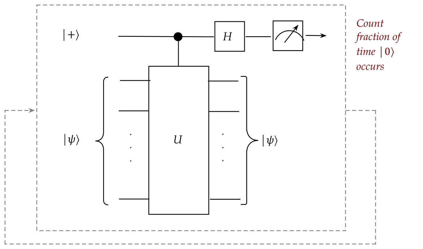
Idea #2: use entanglement
- Here, we will build a controlled-\(U\) circuit and supply
\(\kt{+}\) as the control:
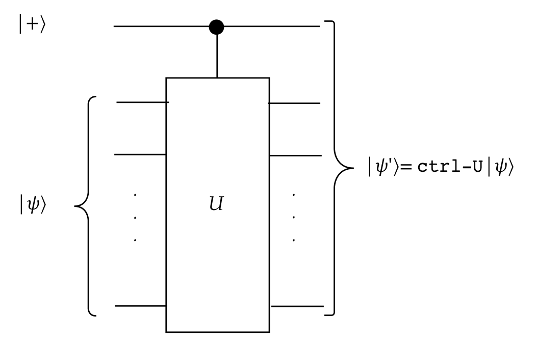
- Recall what controlled-\(U\) does:
- When the control qubit is \(\kt{0}\), no action is taken and
so
$$
\mbox{ctrl-U} \kt{0}\ksi \eql \kt{0} \ksi
$$
- But when the control is \(\kt{1}\), the \(U\) gets applied:
$$
\mbox{ctrl-U} \kt{1}\ksi \eql \kt{1} e^{i\lambda}\ksi
$$
- Thus, when applying \(\kt{+}\)
$$\eqb{
\kt{\psi^\prime} & \eql & \mbox{ctrl-U} \kt{+}\ksi \\
& \eql &
\mbox{ctrl-U} \left(\isqts{1}\kt{0} \; + \; \isqts{1}\kt{1}\right) \ksi \\
& \eql &
\mbox{ctrl-U} \left(\isqts{1} \kt{0}\ksi \; + \; \isqts{1} \kt{1}\ksi \right) \\
& \eql &
\isqts{1} \mbox{ctrl-U} \kt{0}\ksi \; + \; \isqts{1} \mbox{ctrl-U} \kt{1}\ksi\\
& \eql &
\isqts{1} \kt{0}\ksi \; + \; \isqts{1} \kt{1} e^{i\lambda} \ksi\\
& \eql &
\isqts{1} \kt{0}\ksi \; + \; \isqts{1} e^{i\lambda} \kt{1} \ksi\\
& \eql &
\left(\isqts{1} \kt{0} + \isqts{1} e^{i\lambda} \kt{1}\right) \: \ksi\\
}$$
- Now one of the phases in the first qubit has \(\lambda\).
- Note what's unusual:
- Even though \(U\) applies to \(\ksi\), it is the top
qubit that is modified
\(\rhd\)
\(\ksi\) remains the same.
- This happens because of how the phase \(e^{i\lambda}\)
"moves" as a constant in linearity.
- This exploit is called phase-kickback.
- There is no actual physical movement of anything
\(\rhd\)
It's just measurement probabilities that change.
- Could we estimate this through repeated measurements of
the first qubit?
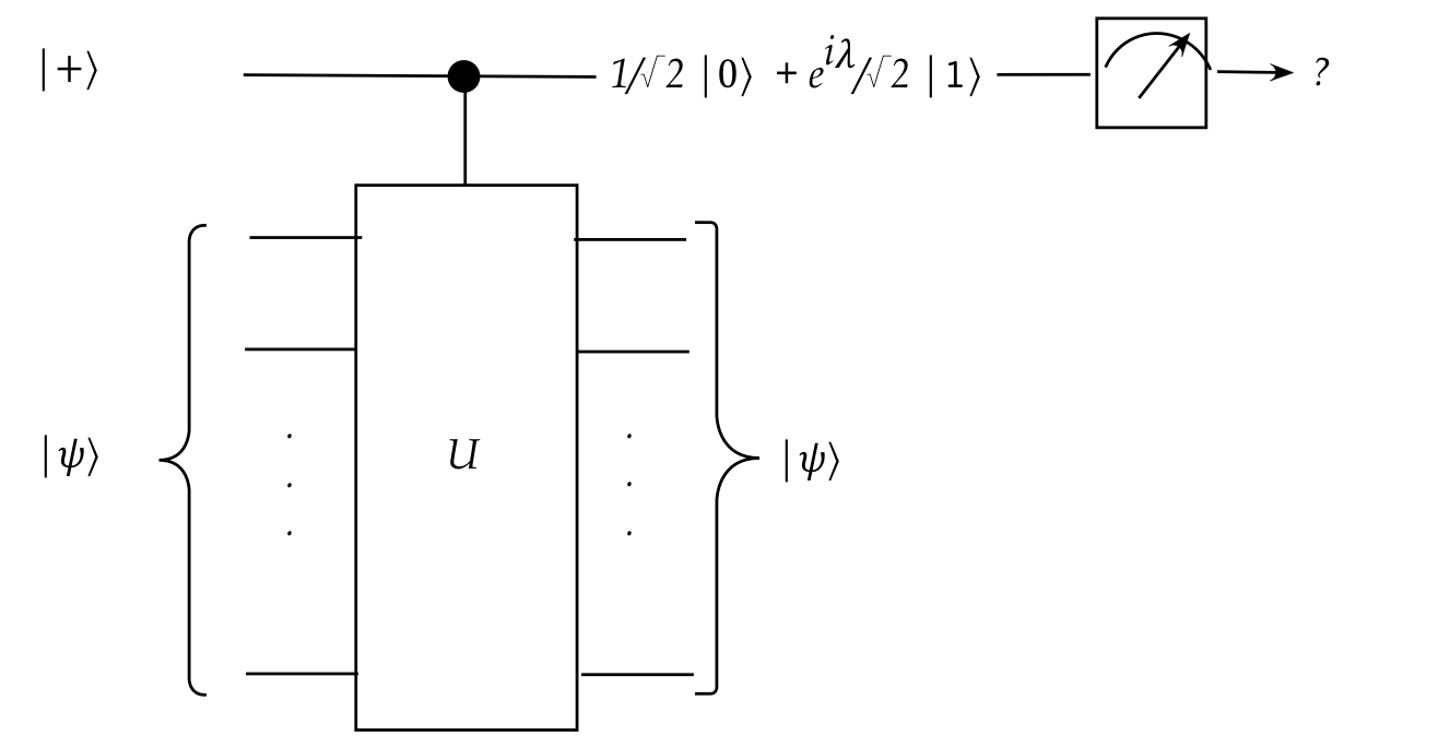
- The probability of observing \(\kt{0}\) is clearly
\(\frac{1}{2}\).
- The probability of observing \(\kt{1}\), therefore, is
also \(\frac{1}{2}\).
\(\rhd\)
Repeated measurements will not help estimate \(e^{i\lambda}\)
(and therefore, possibly, \(\lambda\)).
- We can see this more clearly in the probability for
\(\kt{1}\):
$$
\prob{\mbox{Observe} \kt{1}}
\eql \left| \frac{e^{i\lambda}}{2} \right|^2
\eql \smf{1}{2} \left| e^{i\lambda} \right|^2
\eql \smf{1}{2}
$$
- Could an additional unitary be applied to help?
- The Kitaev and Abrams-Lloyd algorithms differ in how
they do this.
12.5
Kitaev's algorithm
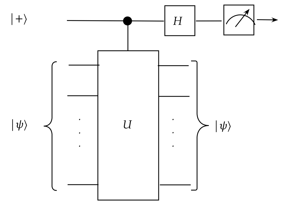
The algorithm does two clever things:
- It applies a simple unitary to the first qubit to
make \(\lambda\) appear differently in
the coefficients of \(\kt{0}\) and \(\kt{1}\).
- This makes the probabilities of \(\kt{0}\) and \(\kt{1}\)
different.
- Then we can estimate any one probability by repeated measurement.
- It makes the reverse engineering of \(\lambda\) easy.
Let's take a closer look:
- The unitary is none other than the go-to unitary: the Hadamard gate
- Recall that, so far, we have
$$
\mbox{ctrl-U} \kt{+}\ksi \eql
\left(\isqts{1} \kt{0} + \isqts{1} e^{i\lambda}
\kt{1}\right) \: \ksi
$$
- Now apply the Hadamard \(H\) (not Hamiltonian!) to the first qubit:
Algebraically,
$$\eqb{
(H \otimes I \otimes \ldots \otimes I) \; \mbox{ctrl-U} \kt{+}\ksi
& \eql &
(H \otimes I \otimes \ldots \otimes I) \;
\left(\isqts{1} \kt{0} + \isqts{1} e^{i\lambda} \kt{1}\right) \: \ksi\\
& \eql &
H \left(\isqts{1} \kt{0} + \isqts{1} e^{i\lambda}
\kt{1}\right) \: \otimes \: (I \otimes \ldots \otimes I) \ksi\\
& \eql &
\left(\isqts{1} H \kt{0} + \isqts{1} e^{i\lambda}
H \kt{1}\right) \: \otimes \: \ksi\\
& \eql &
\left(\isqts{1} \isqts{1} \left(\kt{0}+\kt{1}\right)
\; + \; \isqts{1} e^{i\lambda} \isqts{1} \left(\kt{0} - \kt{1}\right)
\right) \: \otimes \: \ksi\\
& \eql &
\left(\smf{1}{2} \left( 1 + e^{i\lambda} \right) \kt{0}
\; + \; \smf{1}{2} \left( 1 - e^{i\lambda} \right) \kt{1}
\right) \: \otimes \: \ksi\\
}$$
- The first-qubit measurement outcomes (standard basis) are
\(\kt{0}\) and \(\kt{1}\) with probabilities:
$$\eqb{
\prob{\mbox{Observe }\kt{0}}
& \eql & \smf{1}{4} \left| 1 + e^{i\lambda} \right|^2 \\
\prob{\mbox{Observe }\kt{1}}
& \eql & \smf{1}{4} \left| 1 - e^{i\lambda} \right|^2 \\
}$$
- A bit of algebra (see exercise below) shows that
$$\eqb{
\smf{1}{4} \left| 1 + e^{i\lambda} \right|^2
& \eql & \cos^2 \frac{\lambda}{2} \\
\smf{1}{4} \left| 1 - e^{i\lambda} \right|^2
& \eql & \sin^2 \frac{\lambda}{2}
}$$
- Unless \(\frac{\lambda}{2}\) is a multiple of \(\frac{\pi}{4}\), the
two numbers will be different.
- Then, with repeated measurements, one can get
an estimate of, say, the probability of \(\kt{0}\):
- Suppose \(\hat{p}\) is our estimate. Then,
$$
\hat{p} \approx \cos^2 \frac{\lambda}{2} \\
$$
From which
$$
\lambda \approx 2 \cos^{-1} \sqrt{\hat{p}}
$$
In-Class Exercise 1:
Prove the two results
$$\eqb{
\smf{1}{4} \left| 1 + e^{i\lambda} \right|^2
& \eql & \cos^2 \frac{\lambda}{2} \\
\smf{1}{4} \left| 1 - e^{i\lambda} \right|^2
& \eql & \sin^2 \frac{\lambda}{2}
}$$
12.6
QFT review for the Abrams-Lloyd QPE algorithm
In the last module, we showed the following (related) properties of
the QFT:
- First, for any standard-basis vector \(\kt{x} = \kt{x_{n-1}
\ldots x_1 x_0}\):
$$\eqb{
U_{\smb{QFT}} \kt{x}
& \eql &
U_{\smb{QFT}} \kt{x_{n-1} \ldots x_1 x_0}\\
& \eql &
U_{\smb{QFT}} \kt{x_{n-1}} \ldots \kt{x_1} \kt{x_0} \\
& \eql &
\smf{1}{\sqrt{N}}
\left(
\kt{0} \, + \,
\exps{ 2\pi i (0.x_0) } \kt{1}
\right) \\
& &
\; \otimes \;
\left(
\kt{0} \, + \,
\exps{ 2\pi i (0.x_1 x_0) } \kt{1}
\right) \\
& &
\; \otimes \;
\left(
\kt{0} \, + \,
\exps{ 2\pi i (0.x_2 x_1 x_0) } \kt{1}
\right) \\
& & \vdots \\
& &
\; \otimes \;
\left(
\kt{0} \, + \,
\exps{ 2\pi i (0.x_{n-1} \ldots x_0) } \kt{1}
\right)
}$$
- Notice: various (binary) digits of \(x\) appear in
different tensored terms on the right.
- Now consider the inverse QFT applied to the right side:
$$\eqb{
\kt{x_{n-1} \ldots x_1 x_0} & \eql &
U_{\smb{QFT}}^{-1}
\smf{1}{\sqrt{N}}
\left(
\kt{0} \, + \,
\exps{ 2\pi i (0.x_0) } \kt{1}
\right) \\
& &
\; \otimes \;
\left(
\kt{0} \, + \,
\exps{ 2\pi i (0.x_1 x_0) } \kt{1}
\right) \\
& &
\; \otimes \;
\left(
\kt{0} \, + \,
\exps{ 2\pi i (0.x_2 x_1 x_0) } \kt{1}
\right) \\
& & \vdots \\
& &
\; \otimes \;
\left(
\kt{0} \, + \,
\exps{ 2\pi i (0.x_{n-1} \ldots x_0) } \kt{1}
\right)
}$$
This, as expected, produces the original vector \(\kt{x}\).
- Thus, if we wish to extract a number whose digits we
can spread across various qubits as above, we can apply
\(U_{\smb{QFT}}^{-1}\) to recover the number.
- Our goal is to recover the eigenvalue \(\lambda\).
- If we can spread its digits in the pattern above,
we could apply \(U_{\smb{QFT}}^{-1}\).
- This is the goal with the Abrams-Lloyd algorithm.
12.7
The Abrams-Lloyd QPE algorithm
First, let's recall what QPE means:
- Our starting point is a given Hamiltonian \(H\) and one of its
eigenvectors \(\ksi\)
$$
H \ksi = \lambda \ksi
$$
- Then, constructing the unitary \(U=e^{iH}\), we see that
\(\lambda\) appears as a phase:
$$
U \kt{\psi} \eql e^{iH} \kt{\psi} \eql e^{i\lambda} \kt{\psi}
$$
- The goal of QPE (quantum phase estimation) is to estimate
that eigenvalue.
- We will do so by estimating a related number, \(\gamma\), where
$$
\lambda \;\; \approx \;\; 2\pi \gamma
$$
and
$$
\gamma = 0.\gamma_{p-1}\gamma_{p-2}\ldots \gamma_0
$$
is a \(p\)-digit binary number less than \(1\).
(We'll address this assumption below.)
- In particular, because the digits are binary, we'll get these
digits to appear as the bits of a standard-basis vector:
$$
\kt{\gamma_{p-1}} \kt{\gamma_{p-2}} \ldots \kt{\gamma_0}
$$
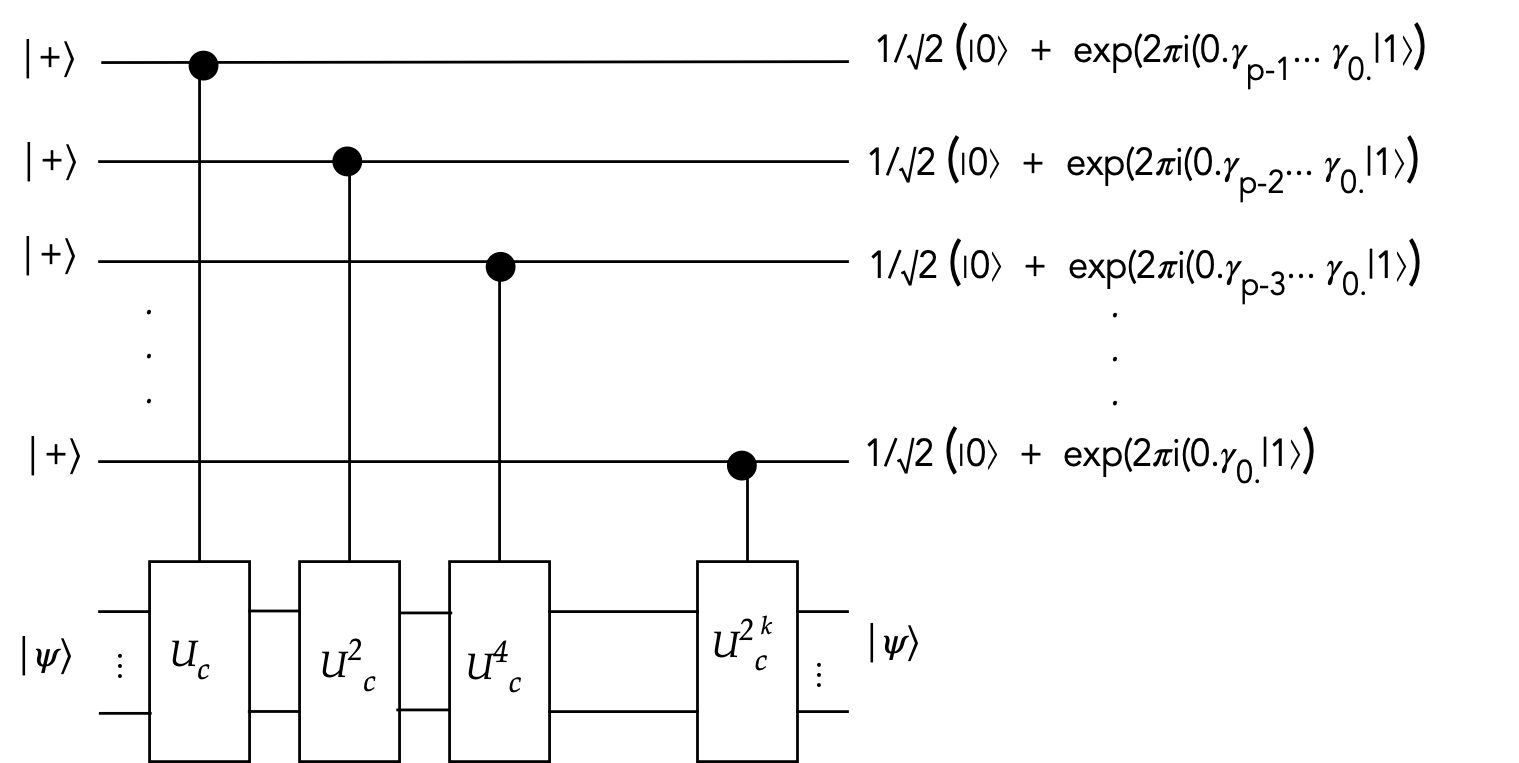
The key ideas:
Summary of the Abrams-Lloyd algorithm:
- Input: the classical simplifed Hamiltonian \(H\) (a Hermitian)
- Define \(U = e^{iH}\) and observe that
$$
U \kt{\psi} \eql e^{i \lambda} \kt{\psi}
$$
which we'll write in terms of a new variable \(\gamma\):
$$
U \kt{\psi} \eql e^{2\pi i \gamma} \kt{\psi}
$$
- Build the quantum circuits for \(U_c^k\)
- Use powers of the controlled version \(U_c^k\) to "kick back" \(e^{2\pi i2^k\gamma}\)
to control qubits.
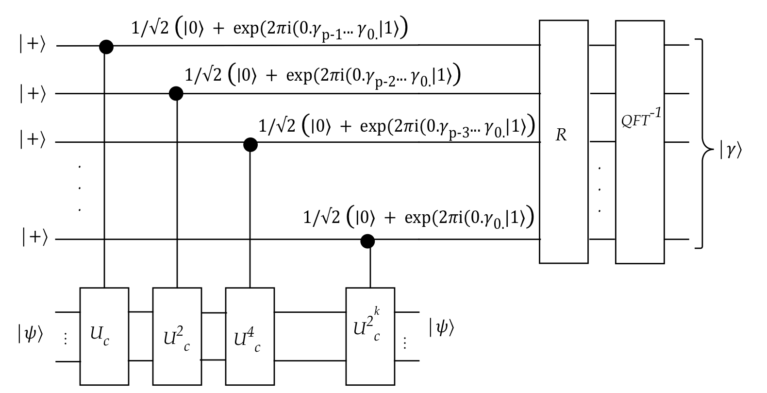
- These (after reversal) are exactly what \(U_{\smb{QFT}}^{-1}\)
needs to produce \(\gamma\) directly as output.
- Once we have \(\gamma\)'s digits, we calculate \(\lambda\).
- Let's condense this into a primitive for future use:

- Here, we're included the Hadamard gates to convert
\(\kt{0}\)'s into \(\kt{+}\)'s.
- We're emphasizing that \(H\) is a classical input.
12.8
Hermitians and measurement for the VQE algorithm
We will focus here on two aspects of measurement useful to the VQE
algorithm:
- The first: single-qubit Pauli measurements
- What does it mean to make a measurement with \(X, Y\) or \(Z\)?
- The second: Pauli-string measurements
- Recall: Hamiltonian simplificaton in terms of Pauli-strings,
for example:
$$\eqb{
H & \approx & \sum_{j=0}^{14} Q_j \\
& \eql &
\alpha_0 I + \alpha_1 Z_1 + \alpha_2 Z_2 + \alpha_3 Z_3 +
\alpha_4 Z_1 Z_2\\
& & + \alpha_5 Z_1 Z_3 + \alpha_6 Z_2 Z4 + \alpha_7 X_1 Z_2 X_3
+ \alpha_8 Y_1 Z_2 Y_3 \\
& & + \alpha_9 Z_1 Z_2 Z_3 + \alpha_{10} Z_1 Z_3 Z_4
+ \alpha_{11} Z_2 Z_3 Z_4 \\
& & + \alpha_{12} X_1 Z_2 X_3 Z_4 + \alpha_{13} Y_1 Z_2 Y_3 Z_4
+ \alpha_{14} Z_1 Z_2 Z_3 Z_4
}$$
- Then for a given state \(\ksi\)
$$\eqb{
\swich{\psi}{H}{\psi} & \eql & \swich{\psi}{\sum_{j} Q_j}{\psi} \\
& \eql & \sum_{j} \swich{\psi}{Q_j}{\psi}
}$$
- Then, for a Pauli string like \(Q_{12} = X_1 Z_2 X_3 Z_4\),
how does one estimate
$$
\swich{\psi}{Q_{12}}{\psi}
\eql \swich{\psi}{X_1 Z_2 X_3 Z_4}{\psi}?
$$
Let's start with single-qubit Pauli measurement:
- Let's consider the connection between Hermitians and measurement.
- We've seen this as:
- Build projectors with the outcomes:
$$
P_i = \otr{\psi_i}{\psi_i}
$$
- Identify the physically observed values \(\lambda_i\)
- Package these into a Hermitian:
$$
A \eql \sum_i \lambda_i \otr{\psi_i}{\psi_i}
$$
- Then, we know that \(A\) has eigenvectors \(\kt{\psi}\)
with eigenvalues \(\lambda_i\).
- We can ask: Is there a measurement corresponding to
any Hermitian matrix \(B\)?
- That is, can we go the other way around?
- This question will only make sense if \(B\)'s
eigenvectors are actual physical outcomes.
- Let's consider an example, first with \(A\)
- Suppose the outcomes are \(\kt{+}, \kt{-}\)
with physical values \(\lambda_1=1, \lambda_2=2\).
- Then,
$$\eqb{
A & \eql & \lambda_1 P_+ \; + \; \lambda_2 P_{-} \\
& \eql & \lambda_1 \otr{+}{+} \;\; + \;\; \lambda_2 \otr{-}{-} \\
& \eql & 1 \otr{+}{+} \; + \; 2 \otr{-}{-} \\
& \vdots & \\
& \eql & \mat{ \frac{3}{2} & -\frac{1}{2} \\
-\frac{1}{2} & \frac{3}{2}} \\
}$$
where \(P_+ = \otr{+}{+}\) and \(P_{-}=\otr{-}{-}\) are the
two projectors.
- Suppose the state of interest is
$$
\ksi \eql \smf{\sqrt{3}}{2} \kt{0} + \smf{1}{2} \kt{1}
$$
- We make repeated measurements and observe the eigenvalues obtained.
- We'd expect the average to be between \(\lambda_1=1, \lambda_2=2\).
- We can calculate this as
$$\eqb{
\swich{\psi}{A}{\psi} & \eql & \exval{\mbox{eigenvalue}}\\
& \eql & \swichs{\psi}{\lambda_1 P_+ + \lambda_2 P_{-}}{\psi} \\
& \vdots & \\
& \eql & 1.067
}$$
- An example of \(10\) actual measurements might be:
\(1,1,2,1,1,1,1,1,1,1\)
\(\rhd\)
Average = \(1.1\)
- Now suppose we're given
$$
B \eql \mat{0 & 1\\ 1 & 0}
$$
- We can certainly calculate \(\swich{\psi}{B}{\psi}\)
- But this may not correspond to feasible measurements with hardware.
- It turns out that \(B\) has the following eigenvectors and values:
$$\eqb{
\kt{+} & \;\;\; & \mbox{with eigenvalue } \lambda_1 = 1
& \mbx{A has eigenvalue \(1\) for this eigenvector}\\
\kt{-} & \;\;\; & \mbox{with eigenvalue } \lambda_2 = -1
& \mbx{A has eigenvalue \(2\) for this eigenvector}\\
}$$
- Thus, the same eigenvectors (but not eigenvalues) as \(A\)
\(\rhd\)
And so, the same projectors (and probabilities)
- How could we estimate average eigenvalue for \(B\)?
- We'll simply measure with \(A\), use its eigenvalues and
make a correspondence with \(B\)'s eigenvalues.
- For example, suppose we get these \(10\) measurements with \(A\):
\(1,1,2,1,1,1,1,1,1,1\)
- We replace these with the corresponding eigenvalues from \(B\):
\(1,1,-1,1,1,1,1,1,1,1\)
- The average is \(0.9\)
- So, our estimate of \(\swich{\psi}{B}{\psi}\) is \(0.9\)
- You noticed that \(B\) is actually the Pauli matrix \(X\).
\(\rhd\)
We now know how to do measurements with \(X\).
- Similarly, one can perform measurements
to estimate \(\swich{\psi}{Y}{\psi}\) or
\(\swich{\psi}{Z}{\psi}\).
- Note that each of \(X,Y,Z\) has eigenvalues \(1,-1\)
but with different eigenvectors:
$$\eqb{
X & \mbox{ has eigenvectors } &
\;\;\;\; \mat{\isqt{1}\\ \isqt{1}} \eql \kt{+}
\;\;\;\; \mbox{ and } \;\;\;\;
\mat{\isqt{1}\\ -\isqt{1}} \eql \kt{-} \\
Y & \mbox{ has eigenvectors } &
\;\;\;\; \mat{\isqt{1}\\ \isqt{i}} \eql \kt{i}
\;\;\;\; \mbox{ and } \;\;\;\;
\mat{\isqt{1}\\ -\isqt{i}} \eql \kt{-i} \\
Z & \mbox{ has eigenvectors } &
\;\;\;\; \kt{0}
\;\;\;\; \mbox{ and } \;\;\;\; \kt{1}
}$$
where \(\kt{i}\) and \(\kt{-i}\) are special names similar
to \(\kt{+}\) and \(\kt{-}\).
In-Class Exercise 2:
Suppose \(\ksi = \alpha\kt{+} + \beta\kt{-}\), with
unknown \(\alpha, \beta\), is a state
for which we wish to estimate the average eigenvalue
with a Pauli-X measurement.
Show how to estimate this eigenvalue using a standard-basis
measurement (that results in eigenvalues \(1, -1\))
applied to \(R_Y(-\frac{\pi}{2})\ksi\).
The second problem to address: estimating the average for a Pauli-string
- Recall, our given Hamiltonian \(H\) is expressed as a sum of
Pauli-string operators, as in:
$$
H \approx \sum_{j} \alpha_j Q_j \\
$$
where, for example, a particular \(Q_j\) might look like this:
$$\eqb{
Q_{7} & \eql & X_1 Z_2 X_3 & \\
& \eql &
\left( X \otimes I \otimes I \right)
& \mbx{\(X\)-measurement on 1st qubit} \\
& \; &
\left( I \otimes Z \otimes I \right)
& \mbx{\(Z\)-measurement on 2nd qubit} \\
& \; &
\left( I \otimes I \otimes X \right)
& \mbx{\(X\)-measurement on 3rd qubit} \\
}$$
- We know how to perform individual qubit measurements, but
what does that imply for these products-of-tensors?
- Suppose our state is (as usual) \(\ksi\).
- Our starting point is
$$
\swich{\psi}{H}{\psi} \eql
\swichs{\psi}{\sum_j \alpha_j Q_j}{\psi}
\eql \sum_j \alpha_j \swich{\psi}{Q_j}{\psi}
$$
where the \(\alpha_j\)'s are known classically.
- Then, for example, we'll need to estimate terms like
$$
\swich{\psi}{Q_7}{\psi}
\eql
\swichh{\psi}{
\left( X \otimes I \otimes I \right)
\left( I \otimes Z \otimes I \right)
\left( I \otimes I \otimes X \right)
}{\psi}
$$
- Here, we'll make the (statistical independence) assumption
$$
\swich{\psi}{Q_7}{\psi}
\eql
\swichh{\psi}{\left( X \otimes I \otimes I \right)}{\psi}
\;
\swichh{\psi}{\left( I \otimes Z \otimes I \right)}{\psi}
\;
\swichh{\psi}{\left( I \otimes I \otimes X \right)}{\psi}
$$
- Finally, examining any of the tensor products, such as the
first one:
$$
\swichh{\psi}{\left( X \otimes I \otimes I \right)}{\psi}
\eql \mbox{average eigenvalue for \(X\)}
$$
Note:
- In general, the eigenvalues of tensored Hermitians are
formed from the products of eigenvalues of the Hermitians.
- Here, the identity matrices have eigenvalue \(1\).
12.9
The VQE Algorithm
Before outlining the algorithm, let's point out:
- Recall, we want to solve
$$
H \kt{\psi_0} \eql \lambda_0 \kt{\psi_0}
$$
where \(\kt{\psi_0}\) is the ground state, and \(\lambda_0\)
is the ground state energy.
- We are going to estimate
$$
\swichs{\psi_0}{H}{\psi_0}
\eql \;\; \mbox{ the ground-state energy }
$$
using \(\kt{\psi} \approx \kt{\psi_0}\):
$$
\swichs{\psi}{H}{\psi}
\eql \;\; \mbox{ approximate ground-state energy }
$$
- \(H\) is fully specified and then decomposed into its
Pauli-string approximation:
$$
H \; \approx \; \sum_j \alpha_j Q_j
$$
where each \(Q_j\) is a Pauli-string operator (a matrix).
- Then,
$$
\mbox{ approximate ground-state energy } \;\;
\eql
\swichs{\psi}{H}{\psi}
\eql \sum_j \alpha_j \swichs{\psi}{Q_j}{\psi}
$$
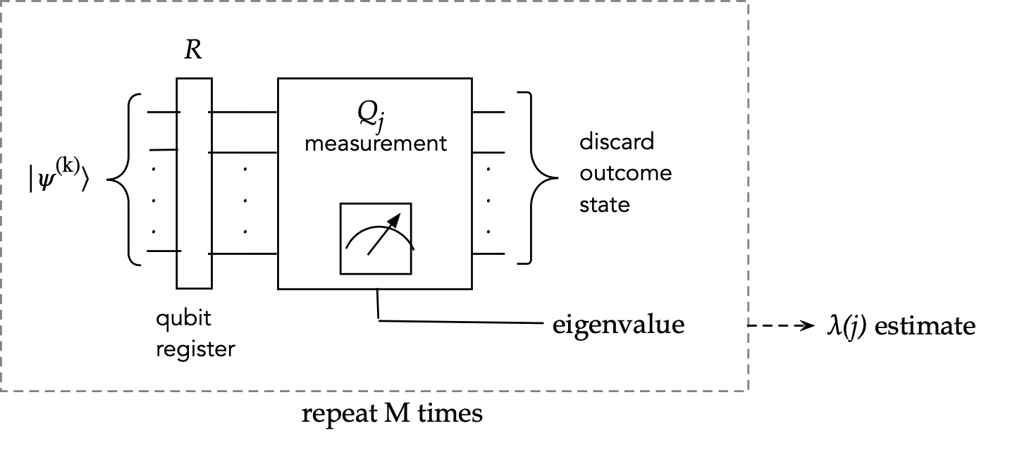
- If we make \(M\) multiple measurements for
\(\swichs{\psi}{Q_j}{\psi}\)
we get a statistical estimate
$$
\hat{\lambda}(j) \eql \smf{1}{M}
\left( \lambda_1(j) + \ldots \lambda_M(j) \right)
$$
These are numbers, one for each \(j\).
- We can put these together into the estimate
$$
\swichs{\psi}{H}{\psi} \; \approx \;
\sum_j \alpha_j \swichs{\psi}{Q_j}{\psi}
\eql
\sum_j \alpha_j \hat{\lambda}(j)
$$
The main idea of the VQE algorithm:
- Step 1: Find a reasonable starting guess
\(\ksi \approx \kt{\psi_0}\).
- Step 2: Estimate \(\lambda\) for current state \(\ksi\):
More precisely:
for each \(j\)
repeat \(M\) times:
(Quantum) Set the state to \(\ksi\)
(Quantum) Perform a single measurement \(\swich{\psi}{Q_j}{\psi}\)
Update the estimate \(\hat{\lambda(j)}\)
Compute final estimate:
\(\hat{\lambda} = \sum_j \alpha_j \hat{\lambda(j)}\)
- Note: the quantum parts are state-setting and measuring.
- Step 3: Update the guess \(\ksi\)
$$
\ksi \; \leftarrow \; \mbox{Better guess}
$$
and return to Step 2.
- Stop the process when no further improvement looks feasible.
Let's now explain a little further in the following way:
- Clearly, steps 2 and 3 are iterative.
- Let
$$
\kt{\psi^{(k)}} \eql \;\; \mbox{\(k\)-th iterate}
$$
That is, the \(\ksi\) used as the \(k\)-th guess for \(\kt{\psi_0}\).
- Then, for Pauli-string \(Q_j\) we use repeated sampling
to estimate \(\swichs{\psi^{(k)}}{Q_j}{\psi^{(k)}}\):
- Next, let's ask: how do we produce a better guess
\(\kt{\psi^{(k+1)}}\)?
- For that matter, how do we even produce the first
guess \(\kt{\psi^{(1)}}\)?
The Ansatz idea for improved guess states:
- Suppose \(R(\theta)\) denotes some (typically rotation) gate
with real-valued parameter \(\theta\).
- Example: \(R_Y(\theta)\), the \(Y\) rotation gate.
- Consider this circuit:
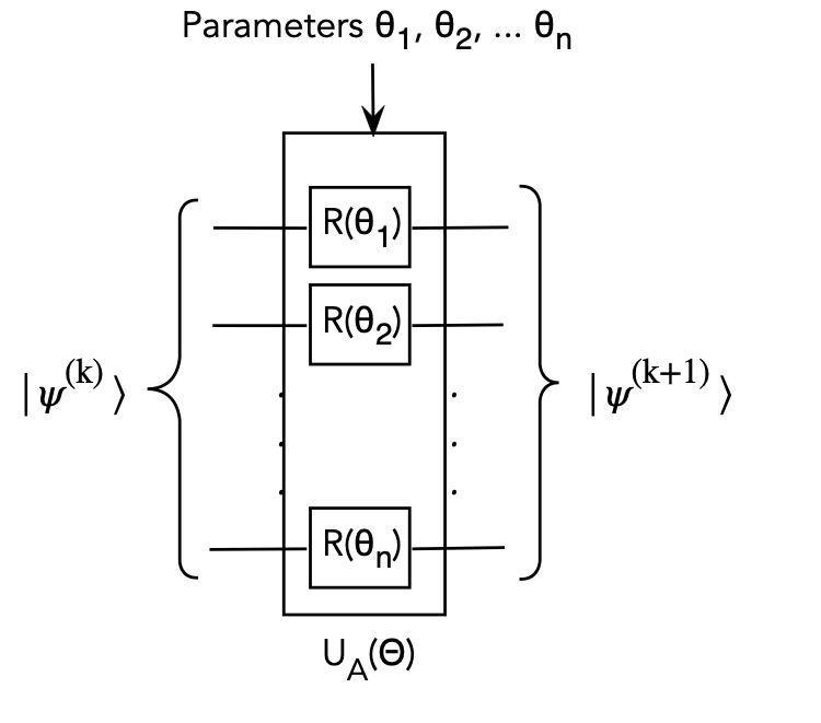
Here
- Each qubit \(k\) can be rotated by a custom gate with a custom
parameter \(\theta_k\).
- Then, the result is a unitary we'll call \(U_A(\Theta)\)
where
$$
\Theta \eql (\theta_1,\ldots, \theta_n)
$$
denotes all the parameters.
- Such a state-producing unitary is called an Ansatz circuit,
which we'll reflect in the subscript as \(U_A\).
- The goal now is to update the parameter set \(\Theta\)
at each iteration:
$$
\Theta^{(k+1)} \eql \mbox{ parameters used to make } \kt{\psi^{(k+1)}}
$$
Improving \(\kt{\psi^{(k+1)}}\) using gradient descent:
- Recall: the goal is to minimize our estimate
$$
\hat{\lambda} \eql \sum_j \alpha_j \hat{\lambda(j)}
$$
where each
$$
\hat{\lambda(j)} \; \mbox{ is an estimate of }
\; \swichs{\psi^{(k)}}{Q_j}{\psi^{(k)}}
$$
- Since \(\kt{\psi^{(k+1)}}\) depends on
\(\Theta^{(k)}\), the parameters used in iteration \(k\)
let's write in the dependence as
$$
\hat{\lambda}(\Theta^{(k)}) \eql \sum_j \alpha_j \hat{\lambda}(j, \Theta^{(k)})
$$
- How do we adjust \(\Theta^{(k)}\)?
- A simple approach is to use gradients.
- Produce estimates
$$\eqb{
\hat\lambda(\theta_1^{(k)},\ldots,\theta_i^{(k)},\ldots, \theta_n^{(k)})
& \;\;\;\;\;\mbox{ estimate using } \theta_i^{(k)}\\
\hat\lambda(\theta_1^{(k)},\ldots,\theta_i^{(k)} + \delta \theta,\ldots, \theta_n^{(k)})
& \;\;\;\;\;\mbox{ estimate using } \theta_i^{(k)} + \delta \theta\\
}$$
- Then
$$\eqb{
\hat{ \frac{ \partial\lambda}{\partial \theta_i} }
& \defn &
\frac{
\hat{\lambda}(\theta_1^{(k)},\ldots,\theta_i^{(k)} + \delta \theta,\ldots, \theta_n^{(k)})
-
\hat{\lambda}(\theta_1^{(k)},\ldots,\theta_i^{(k)},\ldots, \theta_n^{(k)})
}{
\delta \theta
} \\
& \eql &
\;\;\;\;\mbox{partial derivative estimate for parameter \(\theta_i\)}
}$$
- Once these are obtained for each \(\theta_i\), update in the
usual way:
$$
\theta_1^{(k+1)} \eql \theta_1^{(k)} - \gamma
\hat{ \frac{ \partial\lambda}{\partial \theta_i} }
$$
Let's rewrite the VQE algorithm to include these ideas:
- Step 1:
Set \(k=0\)
Find a reasonable starting \(\Theta^{(0)}\)
Set \(\kt{\psi^{(0)}} = U_A(\Theta^{(0)}) \kt{0}\)
- Step 2: Estimate \(\lambda\) for current state
\(\kt{\psi^{(k)}}\)
More precisely:
for each \(j\)
repeat \(M\) times:
(Quantum) Set the state to \(\kt{\psi^{(k)}}\)
(Quantum) Measure a single measurement
\(\swich{\psi^{(k)}}{Q_j}{\psi^{(k)}}\)
Update the estimate \(\hat{\lambda(j)}\)
Compute final estimate for current \(\Theta^{(k)}\):
\(\hat{\lambda}(\Theta^{(k)}) = \sum_j \alpha_j \hat{\lambda(j)}\)
- Step 3: Update \(\Theta^{(k)}\) and apply Ansatz \(U_A\):
$$
\Theta^{(k+1)} \; \leftarrow \;
\mbox{ gradient-based update (Classical calculation)}
$$
and then apply the (quantum) Ansatz with updated parameters:
$$
\kt{\psi^{(k+1)}} \eql U_A(\Theta^{(k+1)}) \: \kt{\psi^{(k)}}
$$
and return to Step 2.
- Stop the process when no further improvement looks feasible.
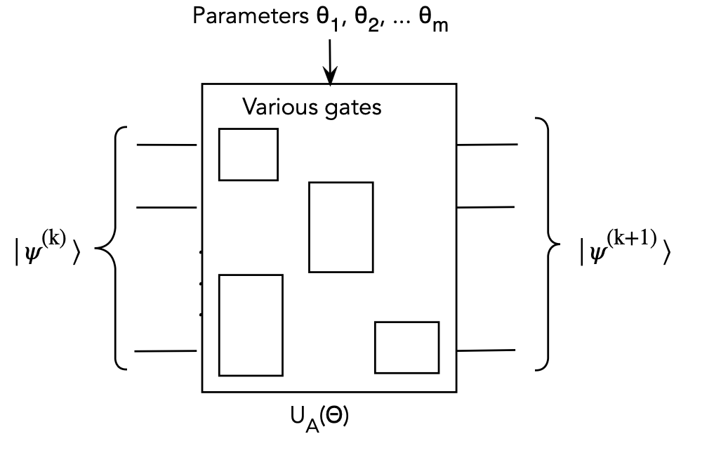
Better Ansatz circuits:
- A fixed set of gates used in the Ansatz limits
expressibility.
- For example, with plain single-qubit rotations, we would not
get any entangled states:
- Thus, one can use a larger set of gates, with 2-qubit \(\cnot\)'s
included:
- There is considerable past and on-going research into
Ansatz design:
- The above approach focuses on expressive hardware (a large
enough family of gates)
- Other approaches exploit problem or application structure.
NISQ and practicalities:
- NISQ = Noisy Intermediate Scale Quantum.
- What this means:
- Today's qubits are noisy and small in number.
- NISQ asks: what problems can we solve in this stage of
quantum computing?
- The VQE algorithm is often proposed as a strong candidate
for NISQ:
- We are making eigenvalue measurements in VQE.
- There is undoubtedly noise, but it cancels in multiple measurements.
- Other practicalities include:
- How to find improved approximations to \(\kt{\psi_0}\)
- How to run the iterative process for maximum benefit.
- Are there other (non-Pauli) measurements that could result in
less noise?
- What is best suited to a particular hardware platform?
- When given a best guess \(\ksi \approx \kt{\psi_0}\),
how does one initialize the qubits to state \(\ksi\)?
All of these are active areas of research.
Generalizing VQE to VQA: Variational Quantum Algorithms
- Consider this description of VQE:
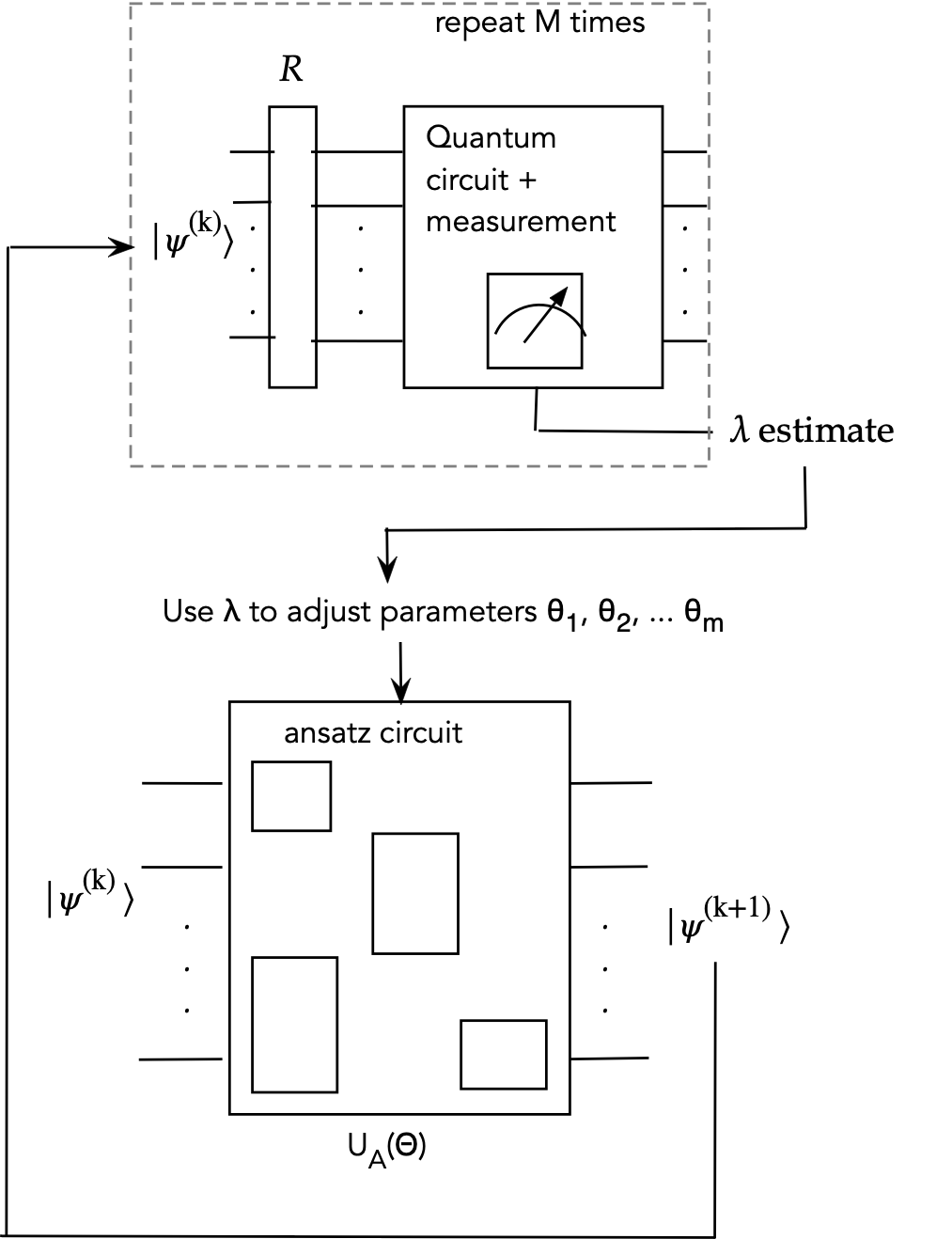
- A quantum ansatz
circuit uses parameters \(\Theta^{(k)}\) at iteration
\(k\) to produce state \(\kt{\psi^{(k)}}\)
- Another quantum circuit (above) is applied to
\(\kt{\psi^{(k)}}\) to eventually produce a measured eigenvalue.
- The goal is to find the minimum eigenvalue.
- The parameters \(\Theta^{(k)}\) are updated using
the measured eigenvalue.
- The next ansatz state is generated:
$$
\kt{\psi^{(k+1)}} \eql U_A(\Theta^{(k)}) \: \kt{\psi^{(k)}}
$$
And one proceeds with the next iteration.
- In essence:
- Classical parameters are used to explore the ansatz
space of \(\kt{\psi^{(k)}}\)'s.
- A different quantum circuit, whose eigenvalue determines
"usefulness" drives the next set of classical parameters.
- This approach can be used to find approximate solutions
to combinatorial problems:
- Suppose a quantum circuit can be designed so that small eigenvalues
correspond to near-optimal solutions to the combinatorial problem.
- Then, the ansatz space can be explored to find approximate solutions.
- This is an area of active research with the Quantum Approximate
Optimization Algorithm (QAOA) as an example approach.
References
The material in this module is summarized from various sources:
- D.S.Abrams and S.Lloyd.
Quantum Algorithm Providing Exponential Speed Increase
for Finding Eigenvalues and Eigenvectors.
Phys. Rev. Lett., 83, 5162, December 1999.
- A.Aspuru-Guzik et al. Simulated Quantum Computation of Molecular
Energies. Science 309, no. 5741: 1704–1707, 2005.
- N.Blunt et al.
A perspective on the current state-of-the-art of quantum computing
for drug discovery applications.
J. Chem. Theory Comput.,18, 12, 7001–7023, 2022.
- K.Brown. Tutorial on Quantum Chemistry Algorithms.
- Cao et al. Quantum Chemistry in the Age of Quantum Computing,
Chemical Reviews, 119, 10856−10915, 2019.
- P.Degelmann, A.Schafer and C.Lennartz.
Application of Quantum Calculations in the Chemical
Industry—An Overview,
International Journal of Quantum Chemistry, 115, 107–136, 2015.
- D.A. Fedorov, B.Peng, N.Govind and Y.Alexeev.
VQE Method: A Short Survey and Recent Developments
Materials Theory, 6, 2, 2022.
- S.Lloyd. Universal Quantum Simulators,
Science, 273, 1996.
- S.McArdle et al. Quantum computational chemistry,
Rev. Mod. Phys., 92, 015003, 2020.
- M.A.Nielsen and I.L.Chuang. Quantum Computation and
Quantum Information, Cambridge University Press, 2016.
- A.Perruzo et al.
A variational eigenvalue solver on a photonic quantum processor.
Nature Communications, Vol. 5, No. 4213, 2014.
- R.Santagati et al.
Drug design on quantum computers, arXiv:2301.04114 [quant-ph].
- J.Tilly et al. The Variational Quantum Eigensolver: a review
of methods and best practices, Physics Reports,
Vol. 986, Pages 1-128, 2022.
- C.P.Williams. Explorations in Quantum Computing, Springer,
2011.