1.1
What is quantum computing and why does it matter?
Currently, the excitement about quantum computing centers on two quite
different applications:
- The promise of faster computation for some problems:
- The prototypical example, the one we will cover, is Shor's
algorithm for fast factorization, which threatens to un-do
parts of conventional cryptography.
- A less hyped but equally important example: fast computation
of molecular properties which will enable designing
molecules (drugs, materials etc).
- The promise of unbreakable security:
- Strange quantum properties allow for two bits to
be entangled so that observation of one bit affects the other.
- Then, if Eve observes a passing bit sent by Alice to Bob,
they'll know.
- This kind of thing just can't be done with conventional hardware.
However, there's an even more important reason that garners little
hype:
- There is a (quiet) revolution underway in the science and
engineering of materials.
- It is now routinely possible in an average lab
to manipulate individual atoms and even their constituent parts.
- And the laws of physics that operate at the atomic and
sub-atomic level are quantum mechanics.
- Thus, it appears reasonable that some form of
quantum phenomena will prevail in the future of computing.
- One could draw an analogy with the steam engine:
- Almost no transportation today operates with steam engines.
- This was not predictable in the early days of steam engines.
- Yet, the steam engine certainly drove innovation in understanding
how to make engines of all kinds, including today's engines.
- Principles developed with steam engines apply broadly to
many kinds of engines.
Note:
This module is a "teaser" module about quantum phenomena for fun and curiosity;
we will not need anything from this module in quantum computing, nor will there be any homework/exam questions.
1.2
Prelude to quantum strangeness: some thought experiments
Gedanken or thought experiments have a long and rich
history in science, especially so in physics.
(Example: Einstein's wondering what it would be like to travel on
a light beam led to a profound altering of physics.)
Let's start with something simpler:
reasoning about pellets fired at a screen:
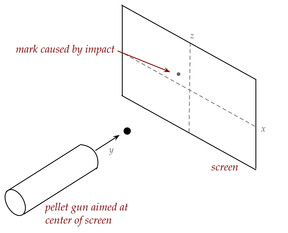
- As is typical in thought experiments, we'll first make
simplifying assumptions and see if the assumptions need to be removed.
- Assume no wind, ignore gravity (because of short range), but
assume that the pellet gun is imperfect in its ejection of the pellet.
- Each pellet hits the screen and leaves a visible mark.
- This leads to a "spread" of dots (marks) on the screen.
\(\rhd\)
"spread" because of imperfections in the pellet gun
- Now suppose we imagine x-y-z axes with the origin at the
center of where the gun is pointed (where a perfectly aimed pellet
would land):

- Next, let's imagine horizontal bands in an area near
the z-axis, as shown, and count how many pellets land in each band.
This will give us a histogram along the z-direction.
In-Class Exercise 1:
What is the shape of the histogram? Draw out a potential histogram
by completing the histogram above. What would we expect to see
with thinner and thinner bands (many of them), and lots of pellets?
If we replaced horizontal bands with vertical bands near the
x-axis to get an x-histogram, what would it look like?
In-Class Exercise 2:
How would your responses change if we placed a hole-in-a-wall
between the gun and the screen?

In-Class Exercise 3:
Now consider moving the pellet gun further back so that
the spread of trajectories is wide enough to encompass
both holes shown here:

What would the x and z histograms look like? And how would those
change if we changed holes to slits? Is it possible for a pellet
that goes through the left slit to land on a spot where a former
right-slit pellet landed?

The next thought experiment will be about randomness:
- Consider these two experiments:
- Flip a coin and observe whether heads or tails faces up.
- Shuffle a deck of cards and examine the top card.
- We often use probabilities to say
- \(\prob{\mbox{heads}} = 0.5 \) (coin flip)
- \(\prob{\mbox{ace of spades}} = \frac{1}{52}\)
(card example)
In-Class Exercise 4:
- What is the source of randomness in each case?
- For the coin-flip,
could one in principle, knowing the launch velocity of the coin
(and other variables), predict the outcome? What variables would be
needed? Could a mechanical contraption be designed to
flip a coin predictably?
- Does this predictability extend to the card example?
- What is an example of a physical measurement that is likely
to have random errors, and for which an average over several
measurements is needed?
For the next thought experiment, we need a bit of background
in magnetism:
In-Class Exercise 5:
How would you describe the motion of the bar magnet?
What is the net force experienced by the center of the bar magnet?
Next, consider the same bar magnet placed in a
magnetic field that's inhomogenous vertically:

- By altering the shape of the larger magnet's South pole, one
can arrange for a greater density of field lines closer to that pole.
- This means the top end of the magnet experiences more
force than the bottom end.
In-Class Exercise 6:
Now how would you describe the motion of the bar magnet?
What is the net force experienced by the center of the bar magnet,
and why? If the orientation of the magnet were changed slightly,
how would that affect the force?
Next, we'll combine the two kinds of experiments (magnet and pellet) by firing
bar magnets through an inhomogenous field:
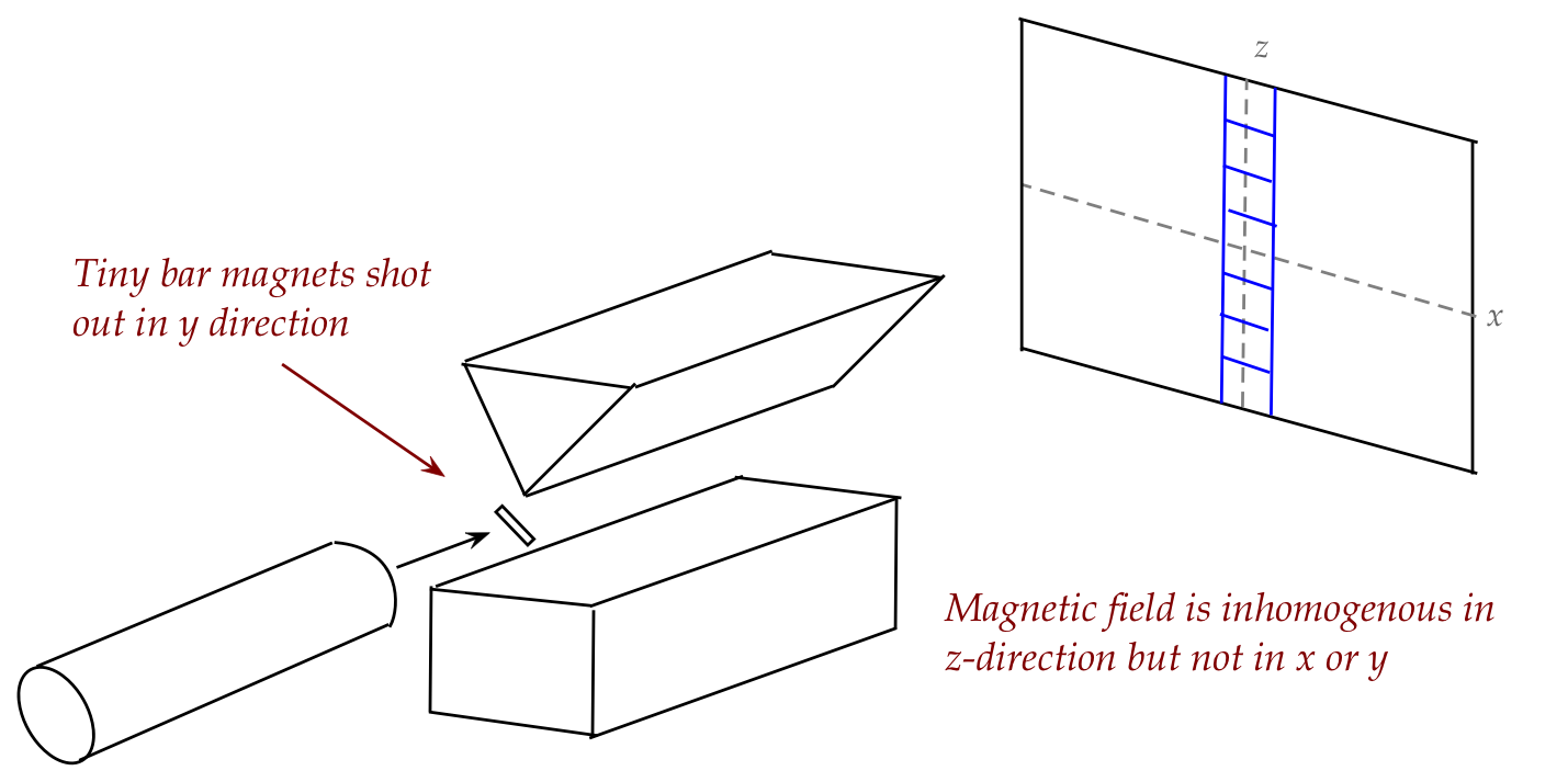
Some assumptions:
- We'll neglect the effects of gravity.
- One tiny bar magnet (a magnetized pellet) is shot out at a
time, letting it hit the screen before the next one is sent.
- The pellet gun cannot control the initial orientation of
a pellet, so assume that over time, pellets are launched at all
kinds of angles, with no bias towards any particular angle.
In-Class Exercise 7:
What does one expect for the z-histogram (vertical),
and why? That is, what is the
histogram going to look like if we count the "hits" in each little
blue box? If one knows the landing spot for a particular bar magnet,
how could one compute the vertical force experienced by the magnet?
What would the histogram look like if the magnetic field were turned off?
The result and explanation above is what one would call
the classical explanation based on what was known between
the time of Newton and the very early 1900's.
1.3
Quantum strangeness: the Stern Gerlach experiment
In 1922, Otto Stern and Walther Gerlach performed their
historic experiment in Frankfurt, Germany:
- Instead of firing small magnets, they launched silver atoms.
- The stream of atoms was produced by heating silver in an
oven, and placing successive barriers with small holes in the way
to create the beam of atoms.
- The detector was a coated glass plate.
- The whole thing was placed in vacuum to prevent air molecules
from interfering with the trajectories of the silver atoms.
- The fundamental assumption about silver atoms at the time:
- They behave like mini magnets, and they emerge from the oven
in a random orientation.
- The thinking was: the outermost electron revolves around the
nucleus, and it was already known that circularly moving electric charges
(a current loop) exhibit magnetic behavior.
- Some interesting historical facts:
- Part of the experiment's funding came from Goldman of
Goldman-Sachs in NY, just based on a request letter.
- A cigar made a difference (improved the visibility of the marks).
- Sadly, Otto Stern had to leave Germany.
So, then, what did Stern-Gerlach discover?

- There are two small vertically separated clusters.
- Based on the center of each cluster, one can calculate
the numeric value of a magnetic property called magnetic
moment. There are only two such values, one positive (the upper
cluster), one negative (the other).
- If we give this a symbol, one could say:
- Atoms in the upper cluster exhibited a magnetic moment of
\(m_B\).
- Atoms in the lower cluster showed a magnetic moment of \(-m_B\).
- The other big observation: the separation is up or down
(along the magnetic field).
- These two observations can be stated more abstractly as:
- The vectorial property called magnetic moment
is quantized in both magnitude and direction.
- Here, quantization means: only particular values occur.
- The magnitude takes on only two values: \(m_B\) or \(-m_B\).
- The direction (orientation) takes on only two values: up or down.
- Another key observation:
if the magnetic field is turned off, the silver atoms behave
just like pellets.
Many questions are now raised:
- Why are there two discrete deflections?
- Are there fundamentally two different kinds of silver atoms?
- Does this happen with other atoms?
Let's answer the last one:
- Yes, it happens with other atoms but with different numbers of
clusters vertically aligned.
- Example: nitrogen shows 4 clusters, sulfer shows 5. All are
along the vertical direction.
In-Class Exercise 8:
What other questions might one ask? What are you curious to know
about this type of experiment?
This is where it starts to get interesting.
We'll use two diagrams to conceptually
simplify depicting the Stern-Gerlach apparatus:

- Assume that the two streams that earlier hit the screen in two
distinct places are now fed through tubes to cleanly separate them
into separate streams.
- The Type-1 diagram above is a conceptual diagram that
simplifies the essence of the input and output streams:
- There's one input port, and two output ports.
- One of the output ports is labeled \({\large +}\) (plus)
to indicate that it's closer to the South end of the field.
- The other is labeled \({\large -}\).
(This is just the naming convention.)
- The diagram can be further conceptually simplifed into the
Type-2 diagram shown that has all the needed info.
- The Type-2 might be harder to use in visualizing, but it
carries all the information about the experimental set up.
1.4
Multi-stage Stern Gerlach experiments
The thought experiment
of examining the output and even subjecting the output to a
further round of magnetic field traversal did not apparently occur to
Stern-Gerlach.
It was in fact the undisputed champion of Gedanken experiments,
Albert Einstein, who proposed it.
Consider the following set up:

In-Class Exercise 9:
Sketch, with modest neatness,
the Type-1 and Type-2 diagrams for a two-stage SG experiment
when the orientation of the second apparatus is
- \(\theta = 0\)
- \(\theta = \pi\)
- \(\theta = \frac{\pi}{2}\)
- \(\theta = \frac{\pi}{4}\)
In-Class Exercise 10:
Sketch Type-1 and Type-2 diagrams for a three-stage SG experiment
where:
- The + output of the first stage is fed into the second.
- The + output of the second stage is fed into a third apparatus.
- The orientations of the three stages are:
\(\theta_1 = 0, \theta_2 = \frac{\pi}{2}, \theta_3 = 0\).
1.5
Stern Gerlach experiments, part I
We'll present results of modern versions
of experiments that came after Stern and Gerlach's original experiment.
Let's start with a closer look at the single stage:

- Assume we can send large numbers of atoms through and carefully
observe where each individual atom exits (+ or -).
- What percentage of atoms exit in the + stream?
\(\rhd\)
Answer: 50% (evenly distributed between + and -).

- Is there a pattern to the exit streams, such as alternate
+ and -?
\(\rhd\)
Answer: It is completely random.
- Do some atoms go elsewhere, somewhere other than the + or
- ports?
\(\rhd\)
Answer: No, all are fully accounted for in the +/- streams.
- Do the observations above change with a different
orientation \(\theta\)?
\(\rhd\)
Answer: No
In-Class Exercise 11:
How does one test that the splitting between two streams is random?
Is it enough to merely establish that 50% exit through the + stream?
We'll next feed the + output into another SG apparatus oriented at \(\theta=0\) :

- The observed output: all the + stream atoms emerge at the +
output of the second stage.
- A similar result obtains from sending the other stream:

- At this point one might reason as follows:
- There are two kinds of atoms, + and -
- The first SG filters out one kind, which is confirmed by the
second SG.
We'll now set the orientation of the second apparatus to align
with the X direction, i.e., \(\theta = \frac{\pi}{2}\):

- Now we see a random split of each + output atom between the
horizontal + and - of the x-aligned second SG.
- A similar result is observed using the - output of the first SG:

- What might one make of this?
- One could argue that there's an "x" property that's randomly
split across atoms, and so, all the "+z" atoms have equal numbers
of "+x" and "-x".
We'll return to two-stage experiments shortly.
We also tweak our diagram to use probabilities instead of
percentages:

- If, over a large number of atoms, the percentage is 25% for a
particular output port, we can
say that the probability for a particular atom to emerge there is 0.25.
- One has to be careful about such statements because we'll
need to assume independence between atoms.
In-Class Exercise 12:
Explore the above notion of independence. Why does it matter?
1.6
Stern Gerlach experiments, part II
The obvious three stage experiments are to use Z-X-Z and Z-X-X:
- Here's the output of Z-X-Z the first with the + output of the
middle SG:

- And again with the other output of the X-aligned SG:

- The pattern of output from the third stage is observed to be
random.
- What are we to make of this?
- Why do "+z" atoms in the first experiment above,
now filtered into "+x" split into "+z" and "-z" in the third stage?
- What is causing the random output in the third stage?
- We can already see that the silver atoms do not carry a "+z" or "-z"
property with them:
- If it were true that each silver atom is either a "+z" kind
or a "-z" kind (but not both), then it can't be that the purely "+z"
stream after the first stage eventually produces "-z" in the third.
1.7
Stern Gerlach experiments, part III
Next, let's point out the observations from two additional variations
of a three-stage set up:
- With some experimental difficulty, it turns out to be possible
to change the direction of an atom stream by \(90^\circ\).
- Then, we can apply a field in the Y direction and observe:

Now for something strange:
- It is possible, overcoming significant experimental challenges,
to merge the two outputs of an SG apparatus:

- The merge is such that every atom
can go either way through the middle X apparatus but appear
at the input of the third.
In-Class Exercise 13:
What is a reasonable guess for the probabilities at two rightmost
outputs? Start by asking: what is the probability that an atom
arrives at the output of the merge apparatus? Then, further,
what is the probability of such an atom to appear at the + output
of the third stage? What is, therefore, the overall probability
that an atom entering the first appears at the + of the third?
[Answer provided in class]
If this wasn't strange enough, consider this variation:

- One could use a faint source of light (photons) to illuminate
which path an atom takes in the merge apparatus.
- Since we can send atoms slowly (one by one) through the
whole apparatus, we can tell which path in the merge an atom takes.
- With this "which path" knowledge, the probabilities observed
change drastically, as shown above.
Even stranger still:
- Suppose one can turn the which-path detector on or off
at will for every atom that passes through the system.
- Then, consider only the subset of atoms when the which-path
is ON:
- For this subset of atoms, the output probabilities are equal
(0.25 each).
- For the other atoms (when which-path is OFF), the
probabilities are 0.5 (+ output) and 0 (for the - output)!
- Let's explain the situation a little further:
- Suppose you turn ON the which-path detector for atoms
1, 3, 4, 6, 10.
- And turn it OFF for atoms 2, 5, 7, 8, 9
- Then, the ON atoms (1, 3, 4, 6, 10) will split probabilistically
evenly between the two outputs.
- This doesn't mean exactly evenly, but applying a coin-flip.
- But every one of atoms 2, 5, 7, 8, 9 will appear on the + output!
1.8
Stern Gerlach experiments, part IV
Now let's return to two-stage SG experiments that will ultimately be
useful in pointing the way forward.
First, consider the second at \(\theta = \pi\):

- Here, the second apparatus is turned through \(180^\circ\) so
that it's upside down.
- The result is that all atoms entering the second come out of
the - port.
In-Class Exercise 14:
To clarify the orientation of the second SG apparatus,
draw the Type-1 diagram for the above case.
Next, consider a general orientation \(\theta\) such as \(\theta =
30^\circ = \frac{\pi}{6}\):
Now let's start with some vague ideas:
- We appear to have properties that are mutually exclusive:
- If one is observed (e.g., +), the other is not (e.g., -)
- If we sought to apply linear algebra, we'd suspect
some kind of orthogonality:

- If a vector \({\bf v}\) is the result of an experiment,
then you can't observe it along a direction
orthogonal to \({\bf v}\).
- This is because \({\bf v}\) has no projection along
the orthogonal direction.
- Next, consider this observation from standard linear algebra:

- Recall that a "+z" stream split evenly between "+x" and "-x".
- Could even projections suggest something similar?
- We know that the projection of \({\bf v}\) along the x-axis
is \(|{\bf v}| \cos(\theta) {\bf e}_1\).
- Yet, we have strange terms like \(\cos^2(\frac{\theta}{2})\)
from experimental observation.
At the moment, it's not clear that linear algebra can explain what
we've observed.
Here are some of the key questions:
- Do atoms carry with them some internal information used to
route them through various SG configurations?
- What accounts for the probabilistic nature of the observed
outputs?
- When the orientation of the second SG is \(\theta =
180^\circ\) why does the output flip signs?
- How does one explain the unexpected results from the merge
apparatus, including the which-path observations?
(And why are we calling this which-path?)
In-Class Exercise 15:
What are your own additional questions?
Before we answer these questions, we will examine another,
very different experimental set up.
Lastly, let's revisit the basic 2-stage SG and point out something.
Recall these two scenarios with a first Z-stage:

- Scenario 1: Second stage is Z-aligned.
- Scenario 2: Second stage is X-aligned.
In-Class Exercise 16:
What is observed when the first stage is an X-aligned SG?

The key observation:
- Think of the second stage as a measuring device.
- For example, in a Z followed by Z, the second Z says
that the stream into the second is 100% (with certainty) a "+z" stream.
- Now consider a Z stage followed by an X stage:
- The X stage output could be either "+x" or "-x".
- There is no certainty involved.
- One could say "certainty in Z" goes with "uncertainty in X",
and vice versa (as shown in the exercise).
\(\rhd\)
We can't have certainty in both Z and X
- This is called the Heisenberg uncertainty principle.
1.9
Experiments with light: background
Light is a complicated subject. We will greatly simplify to present a
few relevant ideas:
The useful phenomenon of polarization:
- Recall our simplified diagram showing the plane of the electric
field in a single wave:

- It is possible for this plane to vary in a single wave, as in:

- Even if individual waves maintained a fixed orientation,
the different waves will have different orientations.
- There are materials that will ensure that all waves that
pass through have a fixed orientation as determined by the material:

-
Note:

- Light that comes out of a polarizer is called polarized light.
- A vertically polarized wave will pass through entirely.
- For waves of other orientation, part will pass through (with
vertical output) and part will be absorbed.
- A horizontally polarized wave will be fully absorbed and
will not get through a vertical polarizer.
- Beam vs. single wave/photon:
- A typical light source will produce many waves (from many
atoms).
- Alternatively: many photons from many atoms.
- A beam is a combination of these.
- Note: we'll later see that it's possible to send a single photon.
- An even more interesting and useful kind of polarizer is
a polarizing beam splitter (PBS):

- When an unpolarized beam arrives, it splits (roughly 50% each)
into two beams that travel in different directions.
- One beam is vertically polarized, the other horizontally polarized.
- A beam splitter merely splits
the input beam into two beams (without polarization):

- One common construction uses a half-silvered mirror.
- Which is why part of the light passes through, and part is reflected.
In-Class Exercise 17:
Consider the following two polarizers in sequence:

What fraction of the input light reaches the other (right) side
of the second polarizer?
In-Class Exercise 18:
Consider inserting a \(45^\circ\) polarizer in the middle:

What fraction of the input light reaches the other (right) side
of the third polarizer?
So now let's turn to the fundamental question about
the nature of light: is it a wave or a photon, or both?
The answer, as it turns out, is surprising.
1.10
Experiments with light: some history
In the early days of physics, Newton thought that light
consisted of small (invisible to the eye) particles:
- His reasoning: waves (such as water and sound) bend around
corners but he did not observe that in light:

- Unfortunately, as he knew, the particle theory did not
explain refraction:

- His contemporary, Christian Huygens, proposed a wave
theory to explain refraction (right side of figure).
Augustin Fresnel's experiment:

- A wave theory would explain bending around an obstacle if
the obstacle is small enough.
The famous double-slit of Thomas Young:
In-Class Exercise 19:
What is the distribution (histogram) expected if both slits are open and
if light is made of particles? What is the height of the
distribution at the center?
The actual distribution with both slits open:

This seems to establish that light is a wave, with the
interference pattern seen with water waves:

Note:
- Think of the screen as "virtual", because a real screen will
involve the waves bouncing back.
- The water molecule at point A moves up and down, away from
its equilibrium.
- The amount of motion (amplitude) depends
on how the two wave shapes add up at point A.
(Two crests will have the highest amplitude. A crest and a
trough will have zero amplitude.)
- The water molecules and points A and B are different.
Enter Einstein:
- He proposed that quantitative observations on the
photoelectric effect could only be explained if
light were quantized, i.e., particles:

- The reasoning:
- If light is all waves, then any frequency should release
electrons, and electrons released should depend on intensity.
- Actual observation: no amount of intensity for
below-threshold frequency light releases any electrons!
- Above the threshold, higher frequency correlates with
electron velocity.
- Thus, if \(E=h\nu\) is energy needed by an electron,
the threshold frequency is \(\nu\) and for \(\nu^\prime \gt \nu\)
the excess energy \(h(\nu^\prime - \nu)\) is converted into
electron kinetic energy.
Many years later, an experiment with very low intensity light:

- A light source that can be made very low intensity.
- If light were a wave, the split should result in
half-intensity in each direction.
- And ... both detectors above should activate, and
simultaneously.
- What actually happens: only one detector goes off.
- Adding up energy used shows no loss anywhere: it's all
accounted for.
- Even more troubling: the detector pattern is random.
Thus, it now looks like light consists of photons.
But what about that double-slit interference pattern?
This is where things start to get strange.
1.11
Experiments with light: Mach-Zehnder interferometry
We'll now examine a series of light-based experiments using
multiple beam splitters.
Let's start with three (non-polarizing) beam splitters
in this configuration:

- Individual photons are released one by one so that
each detection event corresponds to a single photon.
- The probability of transmission (T) is equal to
the probability of reflection (R).
- Each of the four detectors are labeled according to how
an arriving photon underwent transmission and reflection.
- Example: the top most detector RT detects photons that
were reflected (R) at BS1 and then transmitted (T) at BS3.
- Note: once you know which detector went off, the
path from source to that detector is unique.
In-Class Exercise 20:
For a given photon, what is the probability that detector RT
goes off? What are the probabilities for the other detectors?
Next, let's reconfigure the setup slightly:

Note:
- The mirrors are 100% reflective.
- The distance to the top mirror is adjustable, and if increased,
D1 is moved up by the same distance.
In-Class Exercise 21:
For a given photon, what are the probabilities for detecting
at D1 vs D2? Does the adjustable distance matter?
Next, we'll set up what is known at a Mach-Zehnder
interferometer:

Note:
- There is now a beam splitter (BS2) where the two paths cross.
- Thus, a photon arriving at BS2 can be
transmitted or reflected.
- Any photon thus undergoes one of four possibilities at
the two beam splitters (in sequence):
- TT: transmitted through both BS1 and BS2
\(\rhd\)
detected at D2
- RR: reflected through both BS1 and BS2
\(\rhd\)
detected at D2
- RT: reflected at BS1, transmitted at BS2
\(\rhd\)
detected at D1
- TR: transmitted at BS1, reflected at BS2
\(\rhd\)
detected at D1
In-Class Exercise 22:
Based only on the reasoning in the previous two exercises,
what is the probability of detection at D1? At D2?
[Answer provided in class]
Note:
- We are assuming the setup where every photon is sent one at a
time.
- The detection is complete: every detection event
corresponds to a photon (the energies add up correctly).
\(\rhd\)
A "half photon" is never detected
- The distance to the top mirror is adjusted carefully to
make this happen.
- Further adjustments show that one can control the
probabilities of detection at D1 (and therefore at D2).
\(\rhd\)
At another distance, we get the reverse: \(\prob{\mbox{Detect at D2}} \eql 1\)
If this were not strange enough, consider this variation:

- Here, we insert a controllable device that can block a photon.
- This can be turned on and off at will.
- Suppose we now start sending photons and call these
photons 1, 2, 3, ...., 10.
- Next, suppose we apply the block for photons
1, 3, 5, 6, 10 but not for photons 2, 4, 7, 8, 9.
- The photons 1, 3, 5, 6, 10 randomly distribute between D1
and D2.
\(\rhd\)
These are photons for which the path is known.
- The photons 2, 4, 7, 8, 9 all reach D1!
\(\rhd\)
These are photons for which the path is unknown.
- Another way of stating "unknown" is that the paths
are indistinguishable at the second beam splitter.
As we will later see, the fact that paths are indistinguishable
is what is called quantum interference:
- This will turn out to be fundamentally different from
water-wave interference.
- And, even more surprisingly, will turn out to be a
foundation for algorithm design!
1.12
Double-slit revisited
Lastly, let's go back to the historic double-slit experiment
and send in one photon at a time:
\(\rhd\)
An interference pattern is observed.
If one of the slits is closed, one gets the pellet pattern.
It is possible to send larger particles than photons:
- Sending in electrons one at a time results in the
same interference pattern:

- With larger objects, one can detect which slit using
photons:

- But knowing which path now removes interference.
- The double-slit experiment has been performed for
larger particles such as 60-atom molecules, with the same results.
- The fundamental question is: what exactly does a particle do
when confronted with multiple paths?
- Does it pick one randomly?
\(\rhd\)
No, because that would create the two-hump distribution
- Does it go through both?
\(\rhd\)
This seems to defy any conventional notions we have
- Something else?
\(\rhd\)
Indeed. And we'll have more to say about this.
This concludes our first foray into the quantum world:
- As we've seen there are several counter-intuitive outcomes
of experiments.
- Classical (Newtonian) explanations fail to explain these outcomes.
- None of these are easy to understand and have baffled
scientists for over a century when the first such experiments
(Stern-Gerlach) were conducted.
- Note: This introduction was for fun and curiosity:
we don't really need
to understand these experiments to learn quantum computing.
- We will see a few more examples later that will be even
more shocking:
- The delayed-choice experiment.
- The quantum eraser experiment.
- What we will examine and that will a key role
in quantum computing are the underlying foundations that explain what we've seen:
- Complex-number linear algebra: the mathematical elements
- Superposition:
This is the feature that, loosely, explains the
photon taking "two paths" simultaneously.
- Interference: the "wave like" addition/substraction.
- Entanglement: we didn't really see this above, but it
it is yet another unique and baffling quantum property.


