Change of basis
In this review, let's return to two important ideas that
pervade linear algebra: bases and coordinates (in those
bases):
- We'll start by considering a vector as something that can
exist without "numbers" attached to it.
- Then, to "numerify" (if we could coin a term) a vector,
we need to pick a basis.
- The numbers (coordinates) then come from expressing the vector
as a linear combination of the basis vectors.
- We'll go from there to asking whether a matrix-as-operator
itself can be expressed in different bases, and if so, how?
- Finally, if it's true that a matrix can look different in
different bases, then what's the best basis to use?
r.11 Change of basis for vectors
We'll start with a 2D example.
Suppose \(B\) denotes a basis with vectors
\({\bf b}_1\) and \({\bf b}_2\)
where
$$
{\bf b}_1 \eql \vectwo{1}{0}
\;\;\;\;
{\bf b}_2 \eql \vectwo{0}{1}
$$
(This happens to be the standard basis).
Next, suppose \(C\) denotes a basis with vectors
\({\bf c}_1\) and \({\bf c}_2\)
where
$$
{\bf c}_1 \eql \vectwo{2}{4}
\;\;\;\;
{\bf c}_2 \eql \vectwo{3}{1}
$$
Then, if \({\bf u}\) is the vector \((4,3)\), we can
express \({\bf u}\) in either basis:
$$\eqb{
{\bf u} & \eql & 4 {\bf b}_1 + 3 {\bf b}_2
& \eql & 4 \vectwo{1}{0} + 3 \vectwo{0}{1} \\
{\bf u} & \eql & 0.5 {\bf c}_1 + 1 {\bf c}_2
& \eql & 0.5 \vectwo{2}{4} + 1 \vectwo{3}{1} \\
}$$
We can depict both in the following figure:
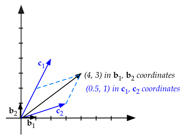
Thus:
- The coordinates of \({\bf u}\) in basis \(B\) are
\((4,3)\).
- The coordinates of \({\bf u}\) in basis \(C\) are
\((0.5,1)\).
We can write these statements in matrix form by placing the basis
vectors as columns:
$$\eqb{
{\bf u} & \eql & \mat{1 & 0\\ 0 & 1} \vectwo{4}{3} \\
{\bf u} & \eql & \mat{2 & 3\\ 4 & 1} \vectwo{0.5}{1} \\
}$$
Next, let us "de-numerify" the vector \({\bf u}\) by removing
all references to a basis and coordinates:
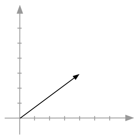
The important point to make is:
- The vector \({\bf u}\) exists (as an arrow) without being
codified numerically in a basis:
- It has a length.
- And it has an orientation (direction).
- To express a vector numerically, we need to pick a
basis.
- The numbers then obtained are the coordinates of the
vector in the basis selected.
- Thus, if we select \(B\) as a basis, then \({\bf u}\)
gets "numerified" as \((4,3)\), the coordinates in \(B\)
(the coefficients in the linear combination).
- If we instead select \(C\), \({\bf u}\)
gets "numerified" as \((0.5, 1)\).
Next, let's ask: if we have the coordinates in one basis, how
can we get the coordinates in another basis?
- Let's start by going from basis \(C\) to basis \(B\) by writing
\({\bf u}\) in \(C\):
$$
\mat{\vdots & \vdots \\
{\bf c}_1 & {\bf c}_2\\
\vdots & \vdots \\}
\vectwo{0.5}{1}
\eql
{\bf u}
$$
We've just put the linear combination into matrix form.
- At this moment, think of the vectors above as
not numerified.
- If we numerify \({\bf c}_1, {\bf c}_2\) and \({\bf u}\)
in the \(B\) basis, we would get:
$$
\mat{2 & 3\\ 4 & 1}
\vectwo{0.5}{1}
\eql
\vectwo{4}{3}
$$
Note:
- How did we write the numbers that comprise the columns of the matrix?
- These are, after all, \({\bf c}_1, {\bf c}_2\).
- The answer: the columns are the vectors \({\bf c}_1, {\bf
c}_2\) numerified in the \(B\) basis.
- That is, the coordinates of \({\bf c}_1, {\bf c}_2\) in the
\(B\) basis.
- Why is this? It's because the un-numerified vectors here
are the two columns \({\bf c}_1, {\bf c}_2\) and the vector
\({\bf u}\) on the right, whereas
0.5 and 1 are the linear-combination-of-columns coefficients.
- This means, whatever basis one picks (like \(B\) above),
we numerify \({\bf c}_1, {\bf c}_2\) and \({\bf u}\),
in that same basis.
-
This converts coordinates in \(C\) to \(B\) coordinates.
- To emphasize, we are going to rewrite this as:
$$
{\bf A}_{C\to B} \;[{\bf u}]_C \eql [{\bf u}]_B
$$
where
$$\eqb{
{\bf A}_{C\to B} & \eql & \mat{2 & 3\\ 4 & 1}
& \eql & \mbox{Change-of-basis matrix from C to B} \\
[{\bf u}]_C & \eql & \vectwo{0.5}{1}
& \eql & {\bf u} \mbox{ expressed in basis C} \\
[{\bf u}]_B & \eql & \vectwo{4}{3}
& \eql & {\bf u} \mbox{ expressed in basis B} \\
}$$
- Thus, we have a way to convert coordinates in one
basis to another.
- To go from \(B\) coordinates to \(C\) coordinates,
there will be some matrix that converts:
$$
{\bf A}_{B\to C} \; [{\bf u}]_B \eql [{\bf u}]_C
$$
-
Clearly, from the earlier conversion of
$$
{\bf A}_{C\to B} \; [{\bf u}]_C \eql [{\bf u}]_B
$$
we can multiply both sides by the matrix inverse to get
$$
[{\bf u}]_C \eql {\bf A}_{C\to B}^{-1} \; [{\bf u}]_B
$$
and so
$$
{\bf A}_{B\to C} \eql {\bf A}_{C\to B}^{-1}
$$
- In this example (once the inverse is found):
$$
\vectwo{0.5}{1}
\eql
\mat{-0.1 & 0.3\\ 0.4 & -0.2}
\vectwo{4}{3}
$$
and so
$$
{\bf A}_{B\to C} \eql \mat{-0.1 & 0.3\\ 0.4 & -0.2}
$$
This is the change-of-basis matrix going from \(B\)
coordinates to \(C\) coordinates.
- Note that the columns
$$
\vectwo{-0.1}{0.3}
\;\;\;\; \mbox{and} \;\;\;\;
\vectwo{0.4}{-0.2}
$$
are the basis vectors of \(B\),
\({\bf b}_1\) and \({\bf b}_2\),
expressed in \(C\)'s coordinates.
Lastly for this section, let's put on our theory hats and
ask: will an inverse exist?
- Since we are working with a basis, the vectors as
columns will be independent.
- Then, if the dimensions are correct, the matrix is square
(with independent columns).
- Thus, the inverse will exist.
To summarize:
- A vector exists without reference to any basis, in which
case it is just a length and a direction.
- To "numerify" a vector, we need to pick a basis, in which
case the numbers are the coordinates in that basis:
the coefficients when expressing the vector as a linear combination
of the basis vectors.
- We now know how to convert coordinates in one basis to
coordinates in another by building the change-of-basis matrix:
- Express the source basis vectors in terms of the target
basis and place these as columns.
- If it's more convenient to start with one basis, then
for the other direction, just use the inverse.
- Having an orthonormal basis simplifies matters because
the inverse is the transpose. Thus,
$$\eqb{
[{\bf u}]_C & \eql & {\bf A}_{C\to B}^{-1} \; [{\bf u}]_B
& \eql & {\bf A}_{C\to B}^{T} \; [{\bf u}]_B
}$$
r.12 Change of basis for matrices
Recall the two meanings of matrix-vector multiplication:
- The vector has the coefficients in the linear combination of
the columns:
$$
\mat{2 & 3\\ 4 & 1\\}
\vectwo{\alpha}{\beta}
\eql
\alpha \vectwo{2}{4}
+
\beta \vectwo{3}{1}
$$
This is the interpretation we use, for example, when we seek
- Change of basis.
- Equation solving (which asks to find the coefficients).
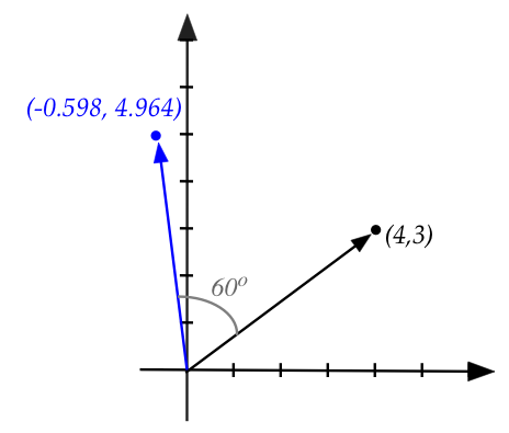
- The other interpretation is that a matrix transforms
one vector into another:
$$
\mat{0.5 & -0.866\\ 0.866 & 0.5}
\vectwo{4}{3}
\eql
\vectwo{-0.598}{4.964}
$$
This happens to be the "rotate anticlockwise by 60 degrees" matrix:
Recall, for a general angle \(\theta\), the rotation matrix turned
out to be:
$$
\mat{\cos(\theta) & -\sin(\theta)\\ \sin(\theta) & \cos(\theta)}
$$
Now let's return to our two bases \(B\) and \(C\) from the earlier
section and ask: does the same transforming matrix work in both?
- That is, we know that in the standard basis \(B\):
$$
\mat{0.5 & -0.866\\ 0.866 & 0.5}
\vectwo{4}{3}
\eql
\vectwo{-0.598}{4.964}
$$
- If we convert \({\bf u} = (4,3)\) to basis \(C\) and
multiply by the rotation matrix, do we get the right result
in \(C\) coordinates?
- First, let's convert the rotated vector to \(C\)
coordinates:
$$
{\bf A}_{B\to C} \vectwo{-0.598}{4.964}
\eql
\mat{-0.1 & 0.3\\ 0.4 & -0.2} \vectwo{-0.598}{4.964}
\eql
\vectwo{1.549}{-1.232}
$$
- We already have calculated \({\bf u} = (0.5,1)\)
in \(C\) coordinates.
- Thus is it true that
$$
\mat{0.5 & -0.866\\ 0.866 & 0.5}
\vectwo{0.5}{1}
\eql
\vectwo{1.549}{-1.232}?
$$
The answer is: no!
- This is because the transforming matrix must also be
converted into \(C\) coordinates.
- If we convert the rotation matrix to \(C\) coordinates
(we'll show how below) we get
$$
\mat{1.366 & 0.866\\ -1.732 & -0.366}
$$
and this gives the correct results:
$$
\mat{1.366 & 0.866\\ -1.732 & -0.366}
\vectwo{0.5}{1}
\eql
\vectwo{1.549}{-1.232}
$$
Let's see how to do this and why it works:
- It is convenient to explain in terms of linear transformations.
- Let \(S\) be a linear transformation. Think of this
abstractly as \(S\) "does something" to a vector:
$$
S({\bf u}) \eql \mbox{some result vector}
$$
For example, \(S\) rotates a vector.
- We know of course that \(S\) gets "numerified" by
representing it as a matrix since every linear transformation
can be expressed as a matrix.
- But for now, let's leave \(S\) as an abstract entity.
(The technical term for this abstraction is operator.)
- Since the basis vectors of \(B\) are vectors, we can build
a matrix by applying \(S\) to these basis vectors
\({\bf b}_1, {\bf b}_2\) and give it a name:
$$
[{\bf A}_S]_B
\defn
\mat{\vdots & \vdots\\
S({\bf b}_1) & S({\bf b}_2)\\
\vdots & \vdots}
$$
where:
- \({\bf A}_S\) means the matrix corresponding to
transformation \(S\).
(We have yet to explain why - see below.)
- The \(B\) subscript emphasizes that we built the matrix \({\bf A}_S\)
using basis vectors from \(B\).
- Next, for any vector \({\bf u}\) expressed in the basis
\(B\), we can write
$$
{\bf u} \eql \alpha_1 {\bf b}_1 + \alpha_2 {\bf b}_2
$$
Here the \(\alpha\)'s are the coordinates of \({\bf u}\)
in basis \(B\).
- By linearity of \(S\):
$$
S({\bf u}) \eql \alpha_1 S({\bf b}_1) + \alpha_2 S({\bf b}_2)
$$
which in matrix form is:
$$
S({\bf u}) \eql
\mat{\vdots & \vdots\\
S({\bf b}_1) & S({\bf b}_2)\\
\vdots & \vdots}
\vectwo{\alpha_1}{\alpha_2}
$$
Or
$$
S({\bf u}) \eql [{\bf A}_S]_B \; {\bf u}
$$
- Thus, the matrix \([{\bf A}_S]_B\) is in fact
the matrix representation of \(S({\bf u})\).
- To emphasise that all of this is occurring in basis
\(B\) we'll use the subscript \(B\) everywhere:
$$
[S({\bf u})]_B \eql [{\bf A}_S]_B \; [{\bf u}]_B
$$
- If everything were converted to basis \(C\) we would
have an equivalent expression
$$
[S({\bf u})]_C \eql [{\bf A}_S]_C \; [{\bf u}]_C
$$
- So, the obvious question is: what is the relation between
\([{\bf A}_S]_C\) and \([{\bf A}_S]_B\)?
- By the definition of \([{\bf A}_S]_C\)
$$
[{\bf A}_S]_C \eql
\mat{\vdots & \vdots\\
[S({\bf c}_1)]_C & [S({\bf c}_2)]_C\\
\vdots & \vdots}
$$
where we're emphasizing that the columns are in \(C\) coordinates.
- Now for a key observation:
$$
[S({\bf c}_i)]_{\bf B} \eql [{\bf A}_S]_{\bf B} \; [{\bf c}_i]_{\bf B}
$$
That is, if we expressed the \({\bf c}_i\)'s in B, then applying
the transformation in \(B\) will give us the \(B\)-version of
the transformed vector.
(We've boldfaced \(B\) to emphasize.)
- But we know how to convert any \(B\) vector to a \(C\)
vector: multiply by the \(B\to C\) change-of-basis matrix:
$$
[S({\bf c}_i)]_{C} \eql {\bf A}_{B\to C} \; [{\bf A}_S]_{B} \; [{\bf c}_i]_{B}
$$
This gives us the i-th column of the transformation matrix in the
\(C\) basis.
- Since matrix-matrix multiplication can be broken down
column by column, we can piece the columns to together:
$$
\mat{\vdots & \vdots\\
[S({\bf c}_1)]_C & [S({\bf c}_2)]_C\\
\vdots & \vdots}
\eql
{\bf A}_{B\to C} \; [{\bf A}_S]_B \;
\mat{\vdots & \vdots\\
[{\bf c}_1]_B & [{\bf c}_2]_B\\
\vdots & \vdots}
$$
- Now for another key observation: the last matrix is
just the \(C\to B\) basis-change matrix!
- And so,
$$
\mat{\vdots & \vdots\\
[S({\bf c}_1)]_C & [S({\bf c}_2)]_C\\
\vdots & \vdots}
\eql
{\bf A}_{B\to C} \; [{\bf A}_S]_B \; {\bf A}_{C\to B}
$$
- Or, more compactly as:
$$
[{\bf A}_S]_C
\eql
{\bf A}_{B\to C} \; [{\bf A}_S]_B \; {\bf A}_{C\to B}
$$
So finally we have a way to convert a transforming
matrix from one basis to another.
- One can use the inverse relation between the two
coordinate change matrices to write this as:
$$
[{\bf A}_S]_C
\eql
{\bf A}_{B\to C} \; [{\bf A}_S]_B \; {\bf A}_{B\to C}^{-1}
$$
Which is less intuitive but compact.
- We have worked it out in 2D but the same reasoning
applies to any dimension.
Let's apply this to our rotation example:
- We have the two change-of-basis matrices:
$$
{\bf A}_{B\to C} \eql
\mat{-0.1 & 0.3\\ 0.4 & -0.2}
\;\;\;\;\;\;
{\bf A}_{C\to B} \eql
\mat{2 & 3\\ 4 & 1}
$$
- Now apply on either side of the rotation (transform) matrix:
$$
\mat{-0.1 & 0.3\\ 0.4 & -0.2}
\mat{0.5 & -0.866\\ 0.866 & 0.5}
\mat{2 & 3\\ 4 & 1}
\eql
\mat{1.366 & 0.866\\ -1.732 & -0.366}
$$
- Finally, apply this new (\(C\)-basis) transform matrix to
to the original vector in \(C\) coordinates:
$$
\mat{1.366 & 0.866\\ -1.732 & -0.366}
\vectwo{0.5}{1}
\eql
\vectwo{1.549}{-1.232}
$$
- As a final check, let's convert the result on the right
back into the \(B\) basis:
$$
{\bf A}_{C\to B}
\vectwo{1.549}{-1.232}
\eql
\mat{2 & 3\\ 4 & 1}
\vectwo{1.549}{-1.232}
\eql
\vectwo{-0.598}{4.964}
$$
- Let's see both bases at work in a single figure:
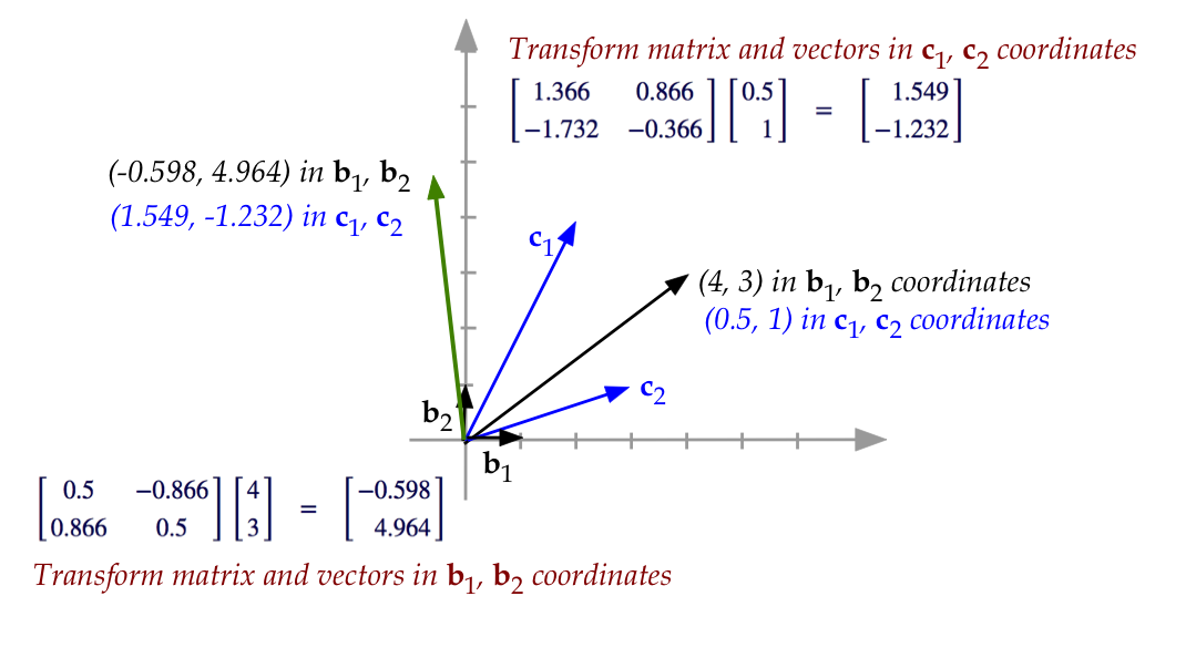
Note:
- The vectors and transform exist without coordinates
(without a basis).
- That is, the start (black) and end (green)
vectors exist as arrows, and therefore one can
speak of a transform that takes one to the other.
- Once we choose a basis, we "numerify" the vectors
and transform.
- If this is all rather confusing, that's understandable.
There's no need to memorize - just remember the highlights
and come back here when you need the details.
r.13 What basis should a (transform) matrix use?
We've seen that a transform can be abstract and then
"numerified" (turned into a matrix) once a basis is selected.
The actual matrix produced is a bunch of numbers, and
you get a different matrix for each choice of basis.
Since we can choose the basis, we should ask: are some
bases better than others for a given transform?
The answer: yes, we should use the eigenbasis if one exists.
Let's consider an example:
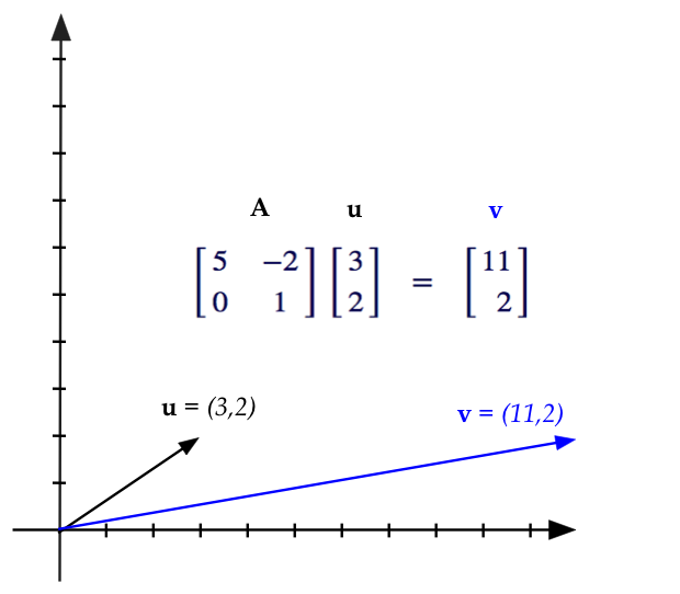
- Let \({\bf A}\) be a transform matrix defined by
$$
{\bf A} \defn \mat{5 & -2 \\ 0 & 1}
$$
- For example, when applied to the vector
\({\bf u} = (3,2)\) we get
$$
{\bf A} {\bf u}
\eql
\mat{5 & -2 \\ 0 & 1} \vectwo{3}{2}
\eql
\vectwo{11}{2}
$$
which we can draw as
- It turns out that \({\bf A}\) has eigenvectors
and corresponding eigenvalues
$$\eqb{
{\bf A} \vectwo{1}{0} & \eql & 5 \vectwo{1}{0} \\
{\bf A} \vectwo{0.5}{1} & \eql & 1 \vectwo{0.5}{1} \\
}$$
- The two eigenvectors are linearly independent (but not orthogonal)
and form a basis.
- Let's call this the \(E\)-basis. And we've called
the standard basis \(B\) in earlier sections.
- Then, let's build the change-of-basis matrix going
from the eigenbasis to standard:
$$
{\bf A}_{E\to B} \eql \mat{1 & 0.5\\0 & 1}
$$
- The inverse (going from \(B\) to \(E\)) turns out to be:
$$
{\bf A}_{B\to E} \eql {\bf A}_{E\to B}^{-1}
\eql \mat{1 & -0.5\\0 & 1}
$$
- Finally, let's convert the transform to its own
eigenbasis, which we'll write as
$$\eqb{
[{\bf A}]_E & \eql & {\bf A}_{B\to E}
\; [{\bf A}]_B \; {\bf A}_{E\to B}\\
& \eql &
\mat{1 & -0.5\\0 & 1} \; \mat{5 & -2 \\ 0 & 1}
\; \mat{1 & 0.5\\0 & 1}
& \eql &
\mat{5 & 0\\0 & 1}
}$$
Which is a diagonal matrix containing the eigenvalues
(and only the eigenvalues).
We've seen this before so let's review (for the general n-dim case):
- Suppose \({\bf A}\) is a transform matrix.
- Suppose \({\bf A}\) has \(n\) eigenvectors
\({\bf x}_1,{\bf x}_2,\ldots,{\bf x}_n\)
and corresponding eigenvalues
\(\lambda_1,\lambda_2,\ldots,\lambda_n\)
where
$$
{\bf A} {\bf x}_i \eql \lambda_i {\bf x}_i
$$
- Then suppose we place the eigenvectors as columns in a matrix
\({\bf E}\)
and the eigenvalues into a diagonal matrix \({\bf \Lambda}\):
$$
{\bf E}
\eql
\mat{ & & & \\
\vdots & \vdots & \vdots & \vdots\\
{\bf x}_1 & {\bf x}_2 & \cdots & {\bf x}_n\\
\vdots & \vdots & \vdots & \vdots\\
& & &
}
$$
and
$$
{\bf \Lambda} \eql
\mat{\lambda_1 & 0 & & 0 \\
0 & \lambda_2 & & 0 \\
\vdots & & \ddots & \\
0 & 0 & & \lambda_n
}
$$
- In Module 12, we showed that
$$
{\bf A E}
\eql
{\bf E \Lambda}
$$
(Notice that the eigenvalue matrix is on the right.)
- If \({\bf E}\) is indeed a basis, it will have
an inverse. Then, we can left-multiply
and switch sides to get:
$$
{\bf \Lambda}
\eql
{\bf E}^{-1} {\bf A} {\bf E}
$$
- Thus, the diagonal eigenvalue matrix can be written
in terms of the eigenbasis matrices.
- But this is exactly the change-of-basis we get
when changing the matrix \({\bf A}\) to
its eigenbasis.
- The take-away: the best basis in which to represent
a transform matrix is the matrix's own eigenbasis (if one exists).
- This last point ("if one exists") is not unimportant:
- The spectral theorem guarantees the existence of such
a basis when \({\bf A}\) is real, symmetric.
We may nonetheless get lucky and get an eigenbasis (as we did
with our running example).
- One additional point: the spectral theorem goes further
and guarantees that if \({\bf A}\) is real and symmetric,
the eigenbasis is orthonormal and the
eigenvalues are real.
- Which means we can write
$$
{\bf \Lambda}
\eql
{\bf E}^{-1} {\bf A} {\bf E}
\eql
{\bf E}^{T} {\bf A} {\bf E}
$$
(since the inverse is just the transpose).
- With our running example of
$$
{\bf A} \defn \mat{5 & -2 \\ 0 & 1}
$$
(which is not symmetric) we nonetheless got lucky and obtained
an invertible
$$
{\bf E} \eql \mat{1 & 0.5\\0 & 1}
$$
Notice: \({\bf E}\) is not orthogonal.
- If, however, we had used a symmetric
$$
{\bf A} \defn \mat{5 & -2 \\ -2 & 1}
$$
we would get
$$
{\bf E} \eql \mat{-0.383 & 0.924\\ -0.924 & -0.383}
$$
which is orthonormal and thus \({\bf E}^T {\bf E} = {\bf I}\)
Lastly, let's examine why eigenvectors are valuable when
considering a transformation \({\bf A}\) applied to any
vector \({\bf u}\):
- Suppose \({\bf A}\) has eigenvectors \({\bf x}_i\) that form a basis.
- Write \({\bf u}\) in terms of this basis:
$$
{\bf u} \eql \sum_i \alpha_i {\bf x}_i
$$
- Now apply \({\bf A}\) to \({\bf u}\):
$$\eqb{
{\bf A} {\bf u} & \eql &
{\bf A} \sum_i \alpha_i {\bf x}_i \\
& \eql &
\sum_i \alpha_i {\bf A} {\bf x}_i \\
& \eql &
\sum_i \alpha_i \lambda_i {\bf x}_i \\
}$$
- This decomposes the action of \({\bf A}\) on \({\bf u}\)
into simple scalar multiplications on the eigenvectors.
Summary:
- When the eigenvectors of a square transform matrix
are linearly independent, one can form a basis using the eigenvectors.
- If the matrix is then converted to eigenbasis coordinates,
the resulting matrix is diagonal.
- The diagonal matrix has two advantages:
- It's easy to compute with (\(n\) values instead of \(n^2\)).
- The diagonal entries neatly separate along dimensions, with
one eigenvalue representing each dimension.
Thus \(n\) numbers describe the entire transformation, and
each number is associated with a different dimension.
- This is why eigenvectors are important: they quantify
the essence of a transformation in its simplest form.