\( \newcommand{\blah}{blah-blah-blah} \newcommand{\eqb}[1]{\begin{eqnarray*}#1\end{eqnarray*}} \newcommand{\eqbn}[1]{\begin{eqnarray}#1\end{eqnarray}} \newcommand{\bb}[1]{\mathbf{#1}} \newcommand{\mat}[1]{\begin{bmatrix}#1\end{bmatrix}} \newcommand{\nchoose}[2]{\left(\begin{array}{c} #1 \\ #2 \end{array}\right)} \newcommand{\defn}{\stackrel{\vartriangle}{=}} \newcommand{\rvectwo}[2]{\left(\begin{array}{c} #1 \\ #2 \end{array}\right)} \newcommand{\rvecthree}[3]{\left(\begin{array}{r} #1 \\ #2\\ #3\end{array}\right)} \newcommand{\rvecdots}[3]{\left(\begin{array}{r} #1 \\ #2\\ \vdots\\ #3\end{array}\right)} \newcommand{\vectwo}[2]{\left[\begin{array}{r} #1\\#2\end{array}\right]} \newcommand{\vecthree}[3]{\left[\begin{array}{r} #1 \\ #2\\ #3\end{array}\right]} \newcommand{\vecfour}[4]{\left[\begin{array}{r} #1 \\ #2\\ #3\\ #4\end{array}\right]} \newcommand{\vecdots}[3]{\left[\begin{array}{r} #1 \\ #2\\ \vdots\\ #3\end{array}\right]} \newcommand{\eql}{\;\; = \;\;} \definecolor{dkblue}{RGB}{0,0,120} \definecolor{dkred}{RGB}{120,0,0} \definecolor{dkgreen}{RGB}{0,120,0} \newcommand{\bigsp}{\;\;\;\;\;\;\;\;\;\;\;\;\;\;\;\;\;\;\;\;\;\;\;\;} \newcommand{\plss}{\;\;+\;\;} \newcommand{\miss}{\;\;-\;\;} \newcommand{\implies}{\Rightarrow\;\;\;\;\;\;\;\;\;\;\;\;} \)

Module 9: Linear Combinations of Other Objects

Part I: Polynomials and Bezier curves

Module objectives

By the end of this module, you should be able to

Explain how other mathematical objects like functions can be placed in linear combinations.

Demonstrate through code, how linear combinations of functions can approximate other functions.

Explain the importance of linear combinations of polynomials.

Explain the connection between polynomials and Bezier curves.

9.0 Linear combinations

Thus far we have worked with linear combinations of vectors:

Given vectors ${\bf v}_1, {\bf v}_2, \ldots, {\bf v}_n$ the vector $$ {\bf b} = x_1 {\bf v}_1 + x_2 {\bf v}_2 + \ldots + x_n {\bf v}_n $$ is a linear combination of the vectors using scalars $x_1,x_2,\ldots,x_n$.

For example: $$ 2 \vecthree{2}{-2}{1} \plss 3 \vecthree{-3}{1}{1} \plss 5 \vecthree{2}{0}{-1} \eql \vecthree{5}{-1}{0} $$ where $x_1=2, x_2=3, x_3=5$.

We've written this in matrix form as: $$ \mat{2 & -3 & 2\\ -2 & 1 & 0\\ 1 & 1 & -1} \vecthree{2}{3}{5} \eql \vecthree{5}{-1}{0} $$

In other words, if matrix ${\bf A}$ has vectors ${\bf v}_1, {\bf v}_2, \ldots, {\bf v}_n$ as columns, then the linear combination $$ {\bf b} = x_1 {\bf v}_1 + x_2 {\bf v}_2 + \ldots + x_n {\bf v}_n $$ is written in our familar matrix form as ${\bf Ax}={\bf b}$.

Given a particular ${\bf b}$ and particular vectors ${\bf v}_1, {\bf v}_2, \ldots, {\bf v}_n$, we know how to solve, or determine whether such a linear combination exists.

We'll now consider linear combinations of objects other than vectors:

That is, we will be interested in $$ \alpha_1 \boxed{\color{white}{\text{LyL}}}_1 + \alpha_2 \boxed{\color{white}{\text{LyL}}}_2 + \ldots + \alpha_n \boxed{\color{white}{\text{LyL}}}_n $$ where mathematical objects other than vectors are in the boxes.
For example, here is a linear combination of $n$ functions that produces a function: $$ g(x) \eql \alpha_1 f_1(x) + \alpha_2 f_2(x) + \ldots + \alpha_n f_n(x) $$

Are such things useful?

Almost all curves in graphics are linear combinations of some kinds polynomials.
$\rhd$ We will see how this works with Bezier curves
Many important functions that are solutions to differential equations are linear combinations of the trig polynomials.
Almost all modern signal processing (sound, images, video) involves some variation of the Discrete Fourier Transform (DFT)
$\rhd$ The DFT is a linear combination of complex vectors.

So, yes, extraordinarily useful.

9.1 Linear combinations of functions: examples

Let's try this example:

Consider the functions $$\eqb{ f_1(x) & \eql & x\\ f_2(x) & \eql & 0\\ f_3(x) & \eql & x^3\\ }$$ and the linear combination $$ g(x) \eql \alpha_1 f_1(x) + \alpha_2 f_2(x) + \alpha_3 f_3(x) $$

We will plot $g(x)$ when $\alpha_1=1, \alpha_2=0, \alpha_3=-\frac{1}{6}$. That is, $$ g(x) \eql x - \frac{1}{6} x^3 $$

In-Class Exercise 1: Download LinCombExample.java and verify that $g(x)$ is being computed as above. Compile and execute to draw the function $g$. You will also need Function.java and SimplePlotPanel.java

So far, nothing interesting.

Next, we'll work towards this linear combination in steps: $$ g(x) \eql x - \frac{1}{6} x^3 + .008333333x^5 - 0.00019841 x^7 + (2.7557\times 10^{-6}) x^9 - (2.50521\times 10^{-8}) x^{11} + (1.605904 \times 10^{-10}) x^{13} $$

In-Class Exercise 2: Download LinCombExample2.java and verify that $g(x)$ is being computed as above. Use different values of n in the program to include additional terms step by step. What is the function $g(x)$ remind you of?

At last we have a useful linear combination.

Let's explore the error between desired and approximate.

In-Class Exercise 3: Download LinCombExample3.java use different values of n to print the error between the approximation function $g(x)$ and the function that $g(x)$ seeks to approximate.

What is the difference in error between n=3 and n=13? What is the ratio?

How does the ratio differ when the interval is $[0,\pi]$ versus $[0,2\pi]$? $[0,\frac{\pi}{2}]$?

Why is the error at each point x multiplied by deltaX, and what does this say about the totalError?

Note:

The functions $f_i(x)$ in the linear combination above were all simple powers of $x$, such as $x^{11}$.
$\rhd$ Each is a simple polynomial, such as $f_{11}(x) = x^{11}$.
It is interesting (and extremely valuable) that a linear combination of simple polynomials results in a very good approximation of a non-polynomial function.
Usually, the smaller the range, the better the approximation.

In-Class Exercise 4: Look up the Taylor series for $sin(x)$. Then, download SinTaylor.java and implement the factorial function. Compare the coefficients printed to those in the alpha[] array used in prior exercises.

Some questions that arise:

Can any function be approximated closely enough by some linear combination of polynomials?
Do the approximating polynomials need to be just the simple powers-of-x, or do they need to be more complex polynomials?
What is a procedure to find the scalars in the linear combination?
Can any of the theory developed for vectors apply to linear combinations of polynomials?
For example: if a collection of "base" polynomials is used in a linear combination, are those basic polynomials linearly independent?

A different kind of example:

We'll now consider linear combinations of trignometric polynomials.
That is, functions like $\sin(k\theta)$.
We'll use a popular variant: $\sin(2\pi k\theta)$.
And, consistent with earlier, notation, we'll write $\sin(2\pi k x)$.
The sum $$ g(x) \eql \sin(2\pi x) + \frac{1}{3}\sin(6\pi x) + \ldots \frac{1}{k} \sin(2\pi kx) $$ is clearly a linear combination of the functions $\sin(2\pi kx)$ for $k=1, k=3, k=5, \ldots$.

In-Class Exercise 5: Download TrigPolyLinComb.java, which ends with k=3. Observe the result. Try adding additional terms until k=11.
Thus, we see that the trig polynomials can be linearly combined to approximate other functions.
But there are limitations too:

In-Class Exercise 6: What is an example of a function $h(x)$ that no linear combination of the different $\sin(2\pi kx)$ functions could possibly approximate?
The same types of questions arise for trig polynomials:
- What types of functions can be approximated closely by trig polynomials?
- What aspects of the theory for vectors port over to linear combinations of trig polynomials?

9.2 Background: approximability

That is, what do we know about whether linear combinations of specialized functions (poly, trig-poly) can approximate a generic function?

Historical background:

Let's trace the arc from the Greek era.

From the Greek era to just before Descartes, mathematics focused on geometry and numbers.

There were symbols, and methods, but much was expressed in language as opposed to the crisp modern notation.

With the arrival of Descartes and symbolic representation of y in terms of x, came functions and functional forms.

For a long while, particular types of functions were studied for their properties:

Example: identities with trigonometric functions.
Example: roots of quadratic functions.

When mathematicians studied properties of functions in general, one of the most basic and important properties turned out to be continuity.
$\rhd$ A continuous function is in some ways "well behaved".

Unfortunately, there are some continuous functions that behave "badly"
$\rhd$ Continuous functions that are nowhere differentiable.

The most celebrated example: Weierstrass' function $$ w(x) \eql \sum_{i=0}^\infty a^i \cos (b^i x) $$ where $a < 1, b > 1, ab \leq 1$.

In-Class Exercise 7: Download Weierstrass.java and execute. Then change the interval as directed.

The function, even though it's linear combination of trig polynomials, is a fractal
$\rhd$ It's not differentiable

Thus, one is led to wonder whether polynomials have any hope of approximating general functions, for two different reasons:

The function being approximated is weird.
But also, linear combinations like the one above could produce weird results.

The first step in this direction was Taylor's theorem (1712), an early post-Newton development in calculus:

Infinitely differentiable functions like $\sin(x)$ can be represented by a Taylor series.
So, differentiating a finite number of times provides an approximation. $$ f(x) \;\;\; \approx \;\;\; f(a) + f'(a)(x-a) + \frac{f''(a)}{2!}(x-a)^2 + \ldots + \frac{f^{(k)}(a)}{k!} (x-a)^k $$
Clearly, by expanding the power, one can write a finite Taylor series as a polynomial.
But, the problem with a Taylor series is that it requires the function being approximated to be differentiable that many times.
Which means it is somewhat "smooth" (a restriction).

The Stone-Weierstrass theorem:

Weierstrass himself, almost a decade later, proved a fundamental result in 1885.
This was later simplified by Marshall Stone in 1948.
Weierstrass was among a group of mathematicians that formalized functions, limits, and other such notions of analysis, as its called.
Let's state it, and then understand what it says.
Theorem: (Stone-Weierstrass) Let $f(x)$ be a continuous function on an interval $[a,b]$. Then, given any $\epsilon > 0$, there is a polynomial $p(x)$ such that $|f(x) - p(x)| < \epsilon$ for all $x\in [a,b]$.
What it's saying:
- We are given the target (continuous) function $f(x)$.
- We are using the notation $p(x)$ to denote polynomial functions, e.g., $p(x) = 1 - 2x + 3x^2 - 4x^7$.
- For any polynomial $p(x)$, the error at the point $x$ is $e(x) = |f(x) - p(x)|$.
- We're looking for a polynomial such that $e(x) < \epsilon$.
- Imagine $\epsilon$ to be small, such as $\epsilon = 0.00001$.
- The theorem says that such a polynomial exists.
A key historical point about the Stone-Weierstrass theorem:
- The proof is not constructive.
- That is, it does not provide a method for constructing $p(x)$.
- It only shows that such a polynomial must exist.
- See for yourself.
Thus, it was a major development when Sergei Bernstein not only provided a constructive proof, but the proof was much simpler.
Berstein's approach used a collection of polynomials as the basis, linear combinations of which approximate a target function.
These special polynomials, in his honor, are called Bernstein polynomials.
And Berstein polynomials, as we'll see, are the foundation of Bezier curves.

9.3 Bernstein polynomials

Definition:

First, recall the Binomial theorem: $$ (x+y)^n = \sum_{k=0}^n \nchoose{n}{k} x^k y^{n-k} $$

Replace $y$ with $1-x$ and define for $x\in [0,1]$ $$ b_{n,k}(x) \;\defn\; \nchoose{n}{k} x^k (1-x)^{n-k} $$ for $k \in \{0,1,2,\ldots,n\}$.

For reasons that will be clear later when we tackle Bezier curves, we'll prefer using $t$ instead of $x$: $$ b_{n,k}(t) \;\defn\; \nchoose{n}{k} t^k (1-t)^{n-k} $$

Note: the polynomials are defined only in the interval $[0,1]$.

They can be scaled and translated to fit the interval $[a,b]$, but that will make the notation ugly.
As it turns out, for Beziers, all we need is the interval $[0,1]$.

For any $n$, there are $n+1$ possible values of $k$ and therefore $n+1$ possible $b_{n,k}(t)$ functions: $$\eqb{ b_{n,0}(t) & \eql & \nchoose{n}{0} t^0 (1-t)^{n-0} & \eql & \frac{n!}{(n-0)! 0!} t^0 (1-t)^{n-0} \\ b_{n,1}(t) & \eql & \nchoose{n}{1} t^1 (1-t)^{n-1} & \eql & \frac{n!}{(n-1)! 1!} t^1 (1-t)^{n-1} \\ b_{n,2}(t) & \eql & \nchoose{n}{2} t^2 (1-t)^{n-2} & \eql & \frac{n!}{(n-2)! 2!} t^2 (1-t)^{n-2} \\ \vdots & & \vdots & & \vdots \\ b_{n,k}(t) & \eql & \nchoose{n}{k} t^k (1-t)^{n-k} & \eql & \frac{n!}{(n-k)! k!} t^k (1-t)^{n-k} \\ \vdots & & \vdots\\ b_{n,n}(t) & \eql & \nchoose{n}{n} t^n (1-t)^{0} & \eql & \frac{n!}{(n-n)! n!} t^n (1-t)^{n-n} \\ }$$

In-Class Exercise 8: What does $\nchoose{n}{k}$ evaluate to in these four cases: $k=0, k=1, k=n-1, k=n$?

If we expand out $t^k (1-t)^{n-k}$, we will get powers of $t$, and therefore, the result is a polynomial (in $t$).

Definition: The $n+1$ functions $b_{n,k}(t) = \nchoose{n}{k} t^k (1-t)^{n-k}$ are called the Bernstein polynomials of degree $n$.

Before proceeding with the Bernsteins, let's explore combinations a bit more.

In-Class Exercise 9: Explain how the formula for $\nchoose{n}{k}$ is derived. Write code in Combinations.java to compute it.

In-Class Exercise 10: Prove that $\nchoose{n}{k} = \nchoose{n-1}{k} + \nchoose{n-1}{k-1}$. Write recursive code in CombinationsRecursive.java to compute it and plot the shape vs. k. Why is it symmetric? Look up Pascal's triangle and draw a few rows. Explain what the above result has to do with Pascal's triangle.

In-Class Exercise 11: Examine CombinationsComparison.java and verify that it compares the number of function calls made in each approach. Try n=5 and n=10 in and explain the disparity in the number of function calls. Then, try n=20 and explain the result.

In-Class Exercise 12: Prove that $\nchoose{n}{k} = \frac{n}{k}\nchoose{n-1}{k-1}$ and implement this approach as a second recursive method in CombinationsComparison2.java. Try n=10 and n=20. Why is the return type double? Implement an iterative version of the above tail recursion.

What are the lessons learned?

A recursive implemention isn't necessarily better, even if it's more elegant.
A recursion that simplifies can be much more efficient.
$\rhd$ Especially if it's a tail recursion that's like an iteration.
Large integers are best represented as long's or double's.

Next, let's explore the Bernstein polynomials.

When $n=1$, there are two Bernstein polynomials: $$\eqb{ b_{1,0}(t) & \eql & 1-t \\ b_{1,1}(t) & \eql & t } $$

In-Class Exercise 13: Copy over your code for combinations into Bernstein.java and plot the two Bernstein polynomials for n=1.
Recall: they are defined only over $[0,1]$.
There are three when $n=2$: $$\eqb{ b_{2,0}(t) & \eql & (1-t)^2 \\ b_{2,1}(t) & \eql & 2t(1-t) \\ b_{2,2}(t) & \eql & t^2 } $$
When $n=3$ $$\eqb{ b_{3,0}(t) & \eql & (1-t)^3 \\ b_{3,1}(t) & \eql & 3t(1-t)^2 \\ b_{3,2}(t) & \eql & 3t^2(1-t) \\ b_{3,3}(t) & \eql & t^3 \\ } $$

In-Class Exercise 14: Plot each family of Bernstein polynomials for n=2 and n=3.

Several questions arise at this point:

Are the Bernstein polynomials a basis?
A basis for what?
What values of $n$ are needed for a basis?
Are they linearly independent?
How does one find linear combinations of Bernsteins to approximate some arbitrary function?
And of course, what does this all have to do with Bezier curves?

Let's get to some of these questions next.

9.4 Properties of Bernstein polynomials

Let's start with a property that will be useful in deriving other properties:

Proposition 9.1: $$ b_{n,k}(t) \eql (1-t) b_{n-1,k}(t) + t b_{n-1,k-1}(t) $$

Before proving this, let's observe that:

The property is analogous to the one we derived for combinations: $$ \nchoose{n}{k} = \nchoose{n-1}{k} + \nchoose{n-1}{k-1} $$ and will in fact use this in the proof.
This will also give us a recursive procedure for computation.

In-Class Exercise 15: Implement the recursive version in Bernstein2.java.

Thus, once again, a recursive procedure may turn out to be less efficient.

For Bezier curves, however, the $n$ is not very high and so a recursive approach is elegant and easier to code.

Furthermore, the recursive approach turns out to have better numerical properties.

Proof of Proposition 9.1: $$\eqb{ RHS & \eql & (1-t) b_{n-1,k}(t) \plss t b_{n-1,k-1}(t)\\ & \eql & (1-t) \nchoose{n-1}{k} t^k (1-t)^{n-1-k} \plss t \nchoose{n-1}{k-1} t^{k-1} (1-t)^{n-1-(k-1)} \\ & \eql & \nchoose{n-1}{k} t^k (1-t)^{n-k} \plss \nchoose{n-1}{k-1} t^k (1-t)^{n-k} \\ & \eql & \left[ \nchoose{n-1}{k} + \nchoose{n-1}{k-1} \right] t^k (1-t)^{n-k} \\ & \eql & \nchoose{n}{k} t^k (1-t)^{n-k} \\ & \eql & b_{n,k}(t) \bigsp\bigsp\bigsp\bigsp\Box }$$

Remember how some of the basic polynomials like $x^3$ can be negative and have strange undulating behavior?

We'll first show that the Bernsteins are all non-negative.

Proposition 9.2: $b_{n,k}(t) \geq 0$ for all $n,k$ and $t\in [0,1]$.

In-Class Exercise 16: For any two numbers $a, b$ such that $ a < b $ and $t\in [0,1]$ prove that $(1-t)a + tb \in [a,b]$. Then, use this fact and Proposition 9.1 to prove 9.2.

Of course, even though they are all non-negative, the coefficients in a linear combination can be negative
$\rhd$ Which will allow approximation of functions that are negative.

Let's now tackle two questions raised earlier:

Q1: Are the Bernstein polynomials a basis?
$\rhd$ That is, can any polynomial be expressed as a linear combination of Bernsteins?
Q2: Are the Bernsteins linearly independent?
First, let's ask what a basis for polynomials might look like.
Consider the "basic" polynomials $$\eqb{ p_0(t) & \eql & 1\\ p_1(t) & \eql & t\\ p_2(t) & \eql & t^2\\ \vdots & \eql & \vdots \\ p_n(t) & \eql & t^n\\ }$$
Let $\mathbb{P}_n$ denote the set of all polynomials of degree $n$ or less.
Any polynomial $p(t)\in \mathbb{P}_n$ can be expressed as a linear combination of these.
- For example, the polynomial $t^2 + t + 41$: $$ t^2 + t + 41 \eql 41 p_0(t) + 1p_1(t) + 1p_2(t) $$
- Similarly, $$ t^5 -15t^4 + 85t^3 -225t^2 -274t - 120 \eql -120p_0(t) -274p_1(t) -225p_2(t) + 85p_3(t) - 15p_4(t) + 1p_5(t) $$
The definition of a generic degree-$n$ polynomial $p(t)$, in fact, is a linear combination of these basic powers-of-t: $$\eqb{ p(t) & \eql & a_0 + a_1t + a_2t^2 + \ldots + a_n t^n\\ & \eql & a_0p_0(t) + a_1p_1(t) + a_2p_2(t) + \ldots + a_np_n(t) }$$
Thus, the basic polynomials $\{p_0(t),\ldots,p_n(t)\}$ form a basis for the set $\mathbb{P}_n$.
Then, Q1 boils down to: do the Bernstein polynomials of degree-n or less also form a basis for $\mathbb{P}_n$?
One restriction: we will limit the interval of definition to $[0,1]$.
First, recall the definition: $$ b_{n,k}(t) \eql \nchoose{n}{k} t^k (1-t)^{n-k} $$
Next, define the collection $$ B_n \eql \{b_{n,0}(t), \;\; b_{n,1}(t), \;\; b_{n,2}(t), \ldots, b_{n,n}(t)\} $$ as the collection of all the Bernsteins of degree n.
For example: $$ B_3 \eql \{ \nchoose{3}{0} (1-t)^3, \;\; \nchoose{3}{1} t(1-t)^2, \;\; \nchoose{3}{2} t^2(1-t), \;\; \nchoose{3}{3} t^3 \} $$
Then Q1 is really asking: is $B_n$ a basis for $\mathbb{P}_n$?
Now define $$ b_{n,k}^\prime(t) \defn t^k (1-t)^{n-k} $$ That is, without the combinatorial term.
Furthermore, define $$ B^\prime_n \eql \{b_{n,0}^\prime(t), \;\; b_{n,1}^\prime(t), \;\; b_{n,2}^\prime(t), \ldots, b_{n,n}^\prime(t) \} $$ For example: $$ B^\prime_3 \eql \{ (1-t)^3, \;\; t(1-t)^2, \;\; t^2(1-t), \;\; t^3 \} $$

In-Class Exercise 17: Write down both $B_n$ and $B^\prime_n$ for $n=1, 2, 3$.
Now, if $B^\prime_n$ is a basis for $\mathbb{P}_n$, then so is $B_n$.

In-Class Exercise 18: Why is this true?
What's left is to argue that $B^\prime_n$ is a basis for $\mathbb{P}_n$:
- This is a slightly tricky argument that uses $B^\prime_n$ and $B^\prime_{n+1}$.
- It'll help to draw the different $B^\prime_n$'s in a sort-of Pascal's triangle:
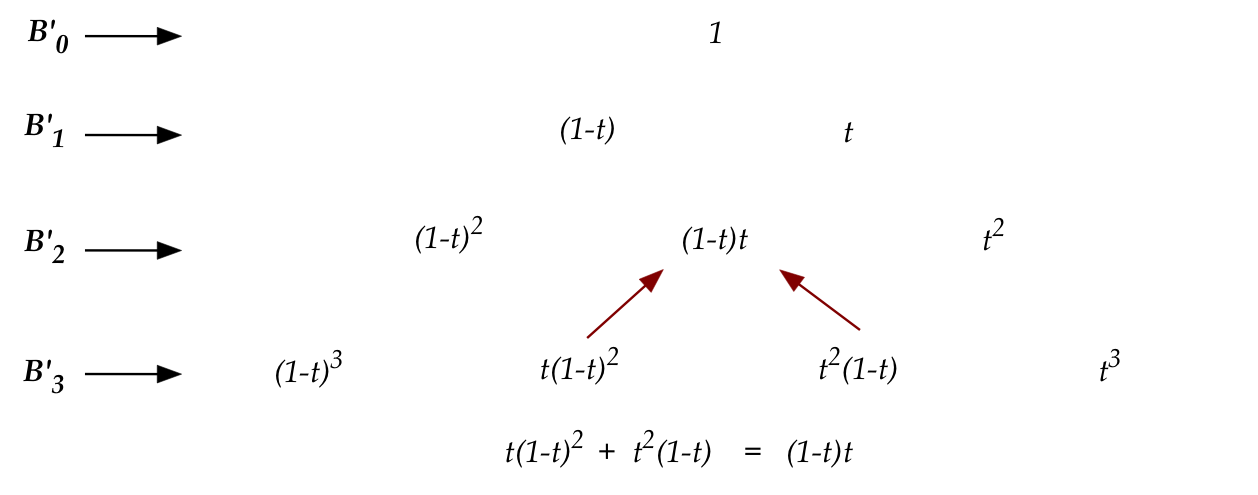
  Here, each $B^\prime_n$ is drawn at a different level.
- Now consider $B^\prime_n$ and $B^\prime_{n+1}$, that is, levels $n$ and $n+1$.
- The k-th term at level n is: $t^k(1-t)^{n-k}$.
- The k-th and (k+1)-st terms at level n are: $t^k(1-t)^{n+1-k}$ and $t^{k+1}(1-t)^{n+1-(k+1)}$.
- We claim: $$ \mbox{ k-th term at level } n \eql \mbox{ k-th term at level } n+1 \plss \mbox{ (k+1)-st term at level } n+1 $$ That is, $$ t^k(1-t)^{n-k} \eql t^k(1-t)^{n+1-k} + t^{k+1}(1-t)^{n+1-(k+1)} $$
  
  In-Class Exercise 19: Prove the above assertion.
- Thus, each element of each row of $B^\prime_n$ can be written in terms of the first n elements of $B^\prime_{n+1}$.
- The last remaining element that was not used from $B^\prime_{n+1}$ in expressing elements from the row above is $t^{n+1}$.
- Now observe that $B^\prime_1$ is a basis for $\mathbb{P}_1$.
  
  In-Class Exercise 20: Why?
- Since each element of $B^\prime_1$ can be expressed by elements of $B^\prime_2$, the span of $B^\prime_2$ includes that of $B^\prime_1$, which is $\mathbb{P}_1$.
- Next, $B^\prime_2$ also includes $t^2$.
- But this is the one additional element needed to span $\mathbb{P}_2$.
- Thus, $B^\prime_2$ spans $\mathbb{P}_2$.
- The same argument repeated for the next two rows shows that $B^\prime_3$ spans $\mathbb{P}_3$.
- Continuing, $B^\prime_n$ spans $\mathbb{P}_n$.
Therefore, from Exercise 18, $B_n$ spans $\mathbb{P}_n$.
The remaining questions are:
- Is $B_n$ minimal?
- Are the elements linearly independent?
Recall that all bases of a space have the same size, which is the dimension.
We know that the dimension of $\mathbb{P}_n$ is $n+1$.
Because $B_n$ has $n+1$ elements, it too is minimal and therefore a basis.
Lastly, Proposition 6.7 showed that elements of a basis are linearly independent.
Whew!

What's left?

A proof that the Bernstein polynomials can closely approximate any function, not just a polynomial.
- This is a bit involved and takes us away from linear algebra, and will be presented separately.
The connection with Bezier curves
- For this purpose, we'll need to understand parametric curve representation first.
Also, Bernstein polynomials have other desirable properties, some numerical. These aren't directly relevant to the course material.

Lastly, since we've seen how linear combinations work for polynomials, let's take a step back and compare polynomials and vectors:

Vectors over the reals Polynomials

Elements They're of the form ${\bf v}=(v_1,v_2,\ldots,v_n)$ They're of the form $p(t) = a_0 + a_1t + a_2t^2 + \ldots + a_nt^n$

Example element ${\bf v}=(1,2,3,4)$ $p(t)= 6 - \frac{9}{5}t - 3t^2 + 4t^3$

Example subspace Subspace in 3D: ${\bf W}=\mbox{span}((-2,2,0), \;(3,3,0))$ Subspace in $\mathbb{P}_3$: ${\bf P}=\mbox{span}(6, 2t, 4t^3)$

Example basis For ${\bf W}$ above: $\{(1,0,0), (0,1,0)\}$. For ${\bf P}$ above: $\{1,t,t^3\}$

Standard basis For all of 3D space: $\{{\bf e}_1=(1,0,0), {\bf e}_2=(0,1,0), {\bf e}_3=(0,0,1)\}$.
For nD: $\{{\bf e}_1, \ldots, {\bf e}_n\}$ where ${\bf e}_i=(0,\ldots,1,\ldots,0)$. For $\mathbb{P}_n$: $\{1,t,t^2,\ldots,t^n\}$.

Linear independence Elements of basis are independent Elements of basis are independent

Alternate bases Any alternative coordinate frame Bernstein polynomials (among others)

9.5 Parametric representation of curves

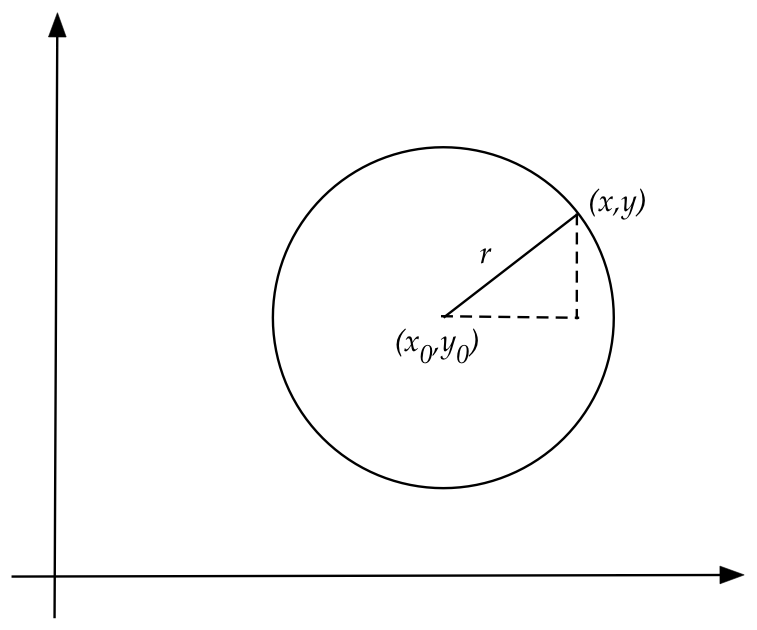
Let's first work with circles:

Recall that the equation for a circle with radius $r$ centered at $(x_0,y_0)$ is $$ (x-x_0)^2 + (y-y_0)^2 \eql r^2 $$

Now consider the process of drawing a circle:

We need a series of closely spaced points.
We'll draw a line between them.

In-Class Exercise 21: Examine the code in DrawCircle.java to see this implemented. Write code to complete the circle. You will also need DrawTool.java.

Observe:

The spacing between points is uneven.
Separate code is needed to handle different square roots of $\sqrt{r^2 - (x-x_0)^2}$.
The code also has to adjust for the start and end of the two segments.

An alternative approach is to recognize that $$\eqb{ x & \eql & x_0 + r\cos\theta\\ y & \eql & y_0 + r\sin\theta }$$ Then, for different values of $\theta$, we will generate points on the circle.

We will prefer using $t$ to $\theta$: $$\eqb{ x & \eql & x_0 + r\cos(t)\\ y & \eql & y_0 + r\sin(t) }$$

In-Class Exercise 22: Write code implementing the above expressions in DrawCircleParametric.java. How can you complete the circle? Change the increment in the $t$ parameter so that you get roughly the same number of points as you had in the previous exercise.

Let's review how this worked by writing $$\eqb{ x(t) & \eql & x_0 + r\cos(t)\\ y(t) & \eql & y_0 + r\sin(t) }$$

Since $t$ is the variable, and $t$ determines $x$ we will write $x(t)$ as a function of $t$.
Similarly, $y(t)$ is a function of $t$.
As $t$ varies, we separately use $x(t)$ and $y(t)$ to compute each point $(x(t), y(t))$.

This is called a parametric representation of a curve:

Here, $t$ is the parameter variable.
In this particular case, a single parameter variable was sufficient, via two functions $x(t)$ and $y(t)$.
One could imagine other curves or surfaces with multiple parameters.
There is no one-right-parametrization for a curve.
$\rhd$ Experience determines what's useful.

Parametric versions exist for many commonly useful curves:

Example: ellipse
- The regular equation for an ellipse centered at $(x_0,y_0)$ is $$ \frac{(x-x_0)^2}{a^2} + \frac{(y-y_0)^2}{b^2} \eql 1 $$
- The parametric version: $$\eqb{ x(t) & \eql & x_0 + a \cos(t) \\ y(t) & \eql & y_0 + b \sin(t) }$$
In-Class Exercise 23: Compile and execute DrawEllipseParametric.java once with and once without the rotation. Then implement translation via matrix multiplication.

In-Class Exercise 24: Compile and execute PlanetaryMotion.java. Observe that the ellipse is rotated about the z-axis. Edit to add rotation about x-axis by $30^\circ$ and then translate by $(2,3,4)$.
Can a straight line be expressed in parametric form?
Consider the well-known form $y = mx + c$:
- We could write $$\eqb{ x(t) & \eql & t \\ y(t) & \eql & mt + c }$$
- This doesn't seem useful
  $\rhd$ It's just the same equation as $y=mx+c$ made unnecessarily more complex.
Instead, consider the line equation when given two points $(x_0,y_0)$ and $(x_1,y_1)$: $$ y \eql y_0 + \frac{(y_1-y_0)}{(x_1-x_0)} (x-x_0) $$
The parametric version is illustrative: $$\eqb{ x(t) & \eql & tx_0 + (1-t)x_1\\ y(t) & \eql & ty_0 + (1-t)y_1 }$$
Initially, let's consider the case $t\in [0,1]$.

In-Class Exercise 25: Compile and execute DrawLineParametric.java. Notice that the computed points are always between the end points.

9.6 Bezier curves

Bezier curves combine two ideas:

Linear combinations of Bernstein polynomials.

Parametric representation of curves

Let's take a look:

As an example, consider the four Bernsteins when $n=3$: $$\eqb{ b_{3,0}(t) & \eql & (1-t)^3 \\ b_{3,1}(t) & \eql & 3t(1-t)^2 \\ b_{3,2}(t) & \eql & 3t^2(1-t) \\ b_{3,3}(t) & \eql & t^3 \\ } $$

A linear combination of the four would look like: $$\eqb{ & \; & a_0 b_{3,0}(t) & + & a_1 b_{3,1}(t) & + & a_2 b_{3,2}(t) & + & a_3 b_{3,3}(t)\\ & \eql & a_0 (1-t)^3 & + & 3a_1 t (1-t)^2 & + & 3a_2 t^2(1-t) & + & a_3 t^3 }$$

A different combination could give us: $$ b_0 (1-t)^3 + 3b_1 t (1-t)^2 + 3b_2 t^2(1-t) + b_3 t^3 $$

Notice that each is a function of $t$.

What if we let one determine $x$ and the other determine $y$?

Let's write this explicitly: $$\eqb{ x(t) & \eql & a_0 (1-t)^3 + 3a_1 t (1-t)^2 + 3a_2 t^2(1-t) + a_3 t^3\\ y(t) & \eql & b_0 (1-t)^3 + 3b_1 t (1-t)^2 + 3b_2 t^2(1-t) + b_3 t^3 }$$

Then, we could draw the curve for different values of $t$:

          for t=0 to 1 step δ
             x = a₀ (1-t)³ + 3a₁ t (1-t)² + 3a₂ t²(1-t) + a₃ t³
             y = b₀ (1-t)³ + 3b₁ t (1-t)² + 3b₂ t²(1-t) + b₃ t³
             plot (x,y)
          endfor

In-Class Exercise 26: Add your code for computing $b_{n,k}(t)$ written earlier into DrawBernsteinParametric.java. Then compile and execute to see the curve drawn.

Next, we will do something unusual:
- We will pair up corresponding coefficients $a_i$ and $b_i$.
- Thus, in the above case we will have $$ (a_0, b_0), \;\;\; (a_1, b_1), \;\;\; (a_2, b_2), \;\;\; (a_3, b_3) $$
- We will treat each of these as a point.
In-Class Exercise 27: Add code to DrawBernsteinParametric2.java to plot the $(a_i,b_i)$ points. You will also need to copy over your code for computing Bernsteins. Then compile and execute to see both the curve and these points.
The points $(a_i,b_i)$ are commonly control points:
- Moving the control points is the same as changing their values
  $\rhd$ Which means changing the curve.
- The number of control points determines the degree of the Berstein polynomials used:
  $\rhd$ There are $n+1$ coefficients for an n-th degree Bernstein family.
In-Class Exercise 28: Add your code for computing Bernsteins to DrawBezier.java. You can now move the points to see how it affects the curve. Increase the number of control points.

Properties of Bezier curves:

Bezier curves have many desirable properties, including:
- The curve will lie within the convex hull of the control points.
- The curve won't "wiggle" more than the control points "wiggle"
  $\rhd$ That is, no more "turns"
- Any straight line will intersect the curve at most as many times as it intersects the line segments between successive control points.
  $\rhd$ Which means the curves behave well between control points.
For proofs of the above, see a book on the mathematics of graphics.

9.7 Bezier surfaces

The Bezier curve idea can be extended to surfaces.

To see how, we'll first write the curve version a little differently:

Recall the control points: $(a_0,b_0), (a_1,b_1),\ldots,(a_n,b_n)$.
Let the i-th control point be written as ${\bf P}_i=(a_i,b_i)$.
Then, recall the $n=3$ example $$\eqb{ x(t) & \eql & a_0 (1-t)^3 + 3a_1 t (1-t)^2 + 3a_2 t^2(1-t) + a_3 t^3\\ y(t) & \eql & b_0 (1-t)^3 + 3b_1 t (1-t)^2 + 3b_2 t^2(1-t) + b_3 t^3 }$$
Now, write this as $$\eqb{ (x(t),y(t)) \eql {\bf P}_0 (1-t)^3 + 3{\bf P}_1 t (1-t)^2 + 3{\bf P}_2 t^2(1-t) + {\bf P}_3 t^3\\ }$$ where it's understood that we are using each control point's coordinates separately.
Thus, the above is just shorthand notation.

The shorthand notation is convenient for generalizing to 3D.

However, there is a small problem to contend with.

At first, it may seem that the natural generalization is: $$\eqb{ (x(t),y(t),z(t)) \eql {\bf P}_0 (1-t)^3 + 3{\bf P}_1 t (1-t)^2 + 3{\bf P}_2 t^2(1-t) + {\bf P}_3 t^3\\ }$$

In-Class Exercise 29: Add your code for computing Bernsteins to Bezier3D_V1.java. First, compile and execute to see where the control points lie. Before taking the next step, try to imagine the surface that the control points are implying, given what you've seen for the 2D case. Next, un-comment the block that computes the surface, compile and execute. What went wrong? Why did it work in 2D but not 3D?

What's needed is a surface.

To get to this, we need an algebraic definition of a surface:

Think of a surface as specified by the height (z value) for every possible (x,y).
Thus, $z=f(x,y)$ defines a surface above the $(x,y)$-plane.

This means, the output of Bezier-surface computation should be a collection of points that define a surface.
$\rhd$ That means, we need two parameters.

Let $W(s,t)$ be the surface defined by parameters $s$ and $t$.

Our goal is to express $W(s,t)$ in terms of the control points, using the control points as coefficients in a linear combination.

This means that it should be possible to vary $s$ and $t$ independently:
$\rhd$ For example: keep $s$ fixed and vary $t$.

But a Bernstein polynomial has only one parameter. What to do?

We really need a Bernstein polynomial with two parameters.

Suppose $b(s,t)$ is such a polynomial then we could take a linear combination using the control points: $$ W(s,t) = \mbox{ linear combination of } b(s,t) \mbox{ functions using control points} $$

There is one more issue to consider: how to describe the control points in a convenient way?
$\rhd$ Should it be a simple array? A list? Something else?

Many surfaces like the one in the example we saw seem to need control points in a grid-like pattern.
$\rhd$ These are more conveniently described as a 2D array, as in the example.

Thus, let's use a 2D grid of 3D points:

${\bf P}_{i,j} = $ the i-j-th point in the grid.
This point could be anywhere in 3D space.
But we expect that ${\bf P}_{i,j}$ will be close in space to points like ${\bf P}_{i+1,j}$ and ${\bf P}_{i,j+1}$.
We therefore want the Bezier surface values to be close for these points as well.

Let's now put these ideas together: $$ W(s,t) \eql \sum_i \sum_j {\bf P}_{i,j} b(s,t) $$

Notice that the linear combination is now written as a double-sum.
This doesn't change the fact that it's a linear combination.
We still have to define $b(s,t)$.

How to define a 2D Bernstein polynomial?

Consider a different problem: what is the 2D version of the curve $f(x)=x^2$?
That is, $f(x,y) = $ 2D version of the square function.
One simple approach: $f(x,y) = x^2 y^2$, a product of squares.

We can now go from $$ b_{n,k}(t) \;\defn\; \nchoose{n}{k} t^k (1-t)^{n-k} $$ to $$ b_{m,i,n,j}(s,t) \;\defn\; \nchoose{m}{i} s^i (1-s)^{m-i} \nchoose{n}{j} t^j (1-t)^{n-j} $$

Finally, we can write $$\eqb{ W(s,t) & \eql & \sum_{i=0}^m \sum_{j=0}^n {\bf P}_{i,j} b_{m,i,n,j}(s,t)\\ & \eql & \sum_{i=0}^m \sum_{j=0}^n {\bf P}_{i,j} \nchoose{m}{i} s^i (1-s)^{m-i} \nchoose{n}{j} t^j (1-t)^{n-j} }$$ Notice:

The grid of control points does not have to be a square grid: m can be different from n.
The 2D Bernstein polynomial is a simple product of the 1D Bernsteins.
The above is a compacted version across the three point dimensions.
Thus, we could write $$\eqb{ x(s,t) & \eql & \sum_{i=0}^m \sum_{j=0}^n {\bf P}_{i,j,x} b_{m,i,n,j}(s,t)\\ y(s,t) & \eql & \sum_{i=0}^m \sum_{j=0}^n {\bf P}_{i,j,y} b_{m,i,n,j}(s,t)\\ z(s,t) & \eql & \sum_{i=0}^m \sum_{j=0}^n {\bf P}_{i,j,z} b_{m,i,n,j}(s,t)\\ }$$ where ${\bf P}_{i,j,x}$ is the x-coordinate of the control point ${\bf P}_{i,j}$.

In-Class Exercise 30: Add your code for computing 2D Bernsteins to Bezier3D.java.

In closing:

Bezier curves and surfaces are just the starting point for a deep dive into the mathematics behind graphics.
Beziers have some advantages:
- They are easy to work with when designing from scratch (as in font design) because moving the control points cause relatively smooth changes in the curves.
- They "behave well" numerically.
However, if you already have a geometric model of an object (such as a cylinder being bent) then you want a curve that will go through its control points, because the control points come from your object's mathematical model.
- In this case, variations of splines like NURBS or Catmull-Rom splines are commonly used.
For rendering efficiently, it is possible to use Chaiken's algorithm to recursively draw segments without actually computing the curve's function.
To browse further:
- See Pixar's introductory tutorial
- Tony DeRose's paper on surface modeling at Pixar. (Layperson story here)

9.8 Approximating any function

Let's revisit an idea from earlier: approximating a function

If the Bernstein polynomials are a basis, a linear combination of the them should be able to approximate any function closely enough.

This in fact was Berntein's original goal and led to his celebrated result.

Let's explore this a bit further.

Let $f(t)$ be any continuous function on $[0,1]$.

Our goal: find scalars $\alpha_k$ such that $$ f(t) \;\; \approx \;\; \sum_{k=0}^n \alpha_k \; b_{n,k}(t) $$

Here, we've picked a particular $n$ and therefore the basis Bernsteins are $b_{n,0}(t), \; b_{n,1}(t), \ldots, b_{n,n}(t)$.

A larger $n$ will allow more basis polynomials, and presumably, a better approximation.

As an example, let's approximate $\sin(2\pi t)$.

In-Class Exercise 31: Add your code for computing bernstein(n,k,t) from earlier to BernsteinApprox.java. Then try different values of n.

Notice that the scalars are very simple to compute: $$ \alpha_k \eql f(\frac{k}{n}) $$ In other words:

The function $f$ is evaluated at $n+1$ equidistant points along $[0,1]$.
That is: $f(0), \; f(\frac{1}{n}), \; f(\frac{2}{n}), \ldots, f(\frac{n}{n}) $

Another way of thinking about it:

Suppose we had data consisting of $n+1$ points evaluated at equidistant points along $[0,1]$.
Here, there's only data, and no known function.
A reasonable approximation is to use the $n$-basis of Bernstein polynomials to approximate that data with a function.
The scalars in the linear combination are just the data themselves.
It couldn't get simpler!

The remarkable result that Bernstein proved: for any continuous, bounded function $f$ on $[0,1]$ $$ \lim_{n\rightarrow\infty} \sum_{k=0}^n f(\frac{k}{n}) b_{n,k}(t) \eql f(t) $$

See example proofs: here and here

	Vectors over the reals	Polynomials
Elements	They're of the form \({\bf v}=(v_1,v_2,\ldots,v_n)\)	They're of the form \(p(t) = a_0 + a_1t + a_2t^2 + \ldots + a_nt^n\)
Example element	\({\bf v}=(1,2,3,4)\)	\(p(t)= 6 - \frac{9}{5}t - 3t^2 + 4t^3\)
Example subspace	Subspace in 3D: \({\bf W}=\mbox{span}((-2,2,0), \;(3,3,0))\)	Subspace in \(\mathbb{P}_3\): \({\bf P}=\mbox{span}(6, 2t, 4t^3)\)
Example basis	For \({\bf W}\) above: \(\{(1,0,0), (0,1,0)\}\).	For \({\bf P}\) above: \(\{1,t,t^3\}\)
Standard basis	For all of 3D space: \(\{{\bf e}_1=(1,0,0), {\bf e}_2=(0,1,0), {\bf e}_3=(0,0,1)\}\). For nD: \(\{{\bf e}_1, \ldots, {\bf e}_n\}\) where \({\bf e}_i=(0,\ldots,1,\ldots,0)\).	For \(\mathbb{P}_n\): \(\{1,t,t^2,\ldots,t^n\}\).
Linear independence	Elements of basis are independent	Elements of basis are independent
Alternate bases	Any alternative coordinate frame	Bernstein polynomials (among others)