Module objectives
By the end of this module, you should be able to
- Describe and interpret a few key theoretical results
in linear algebra.
- Describe how one of the results applies to least-squares.
- Describe a linear transformation and its relationship
to matrices.
Before we start, let's review the two different meanings
of dimension:
- The dimension of a vector is the number of
components in that vector.
- This is same as in the commonly used phrases 2D or 3D.
- Examples:
$$
\vectwo{1}{-2}
$$
is two-dimensional whereas
$$
\vecthree{-1.5}{2}{4.6}
$$
is three-dimensional.
- The dimension of a subspace (which is a set, not a
single thing) is the number
of vectors in a basis for that subspace.
- This is asking: what is the minimum number of vectors
(how many vectors) needed to span a given subspace.
- Example: suppose \({\bf W} = \{(x_1,x_2,0): x_i\mbox{ is real}\}\)
- \({\bf W}\) is a space consisting of three-component vectors.
- How many vectors are needed to span \({\bf W}\)?
- The two vectors \({\bf u}=(1,0,0)\) and \({\bf v}=(0,1,0)\)
are sufficient but any one vector all by itself is not.
- Thus the dimension of \({\bf W}\) is 2.
- We write this as \(\mbox{dim}\;{\bf W} = 2\).
If this were not confusing enough, one also speaks of the
dimensions (plural) of a matrix: the number of rows and the
number of columns.
8.0
What is a fundamental theorem?
In-Class Exercise 1:
Type the search term "fundamental theorem of a" to see
suggested completions, then try "fundamental theorem of b",
and so on. What is the first letter that fails?
About fundamental theorems:
- Clearly, the world is rife with fundamental theorems.
- Somehow, a fundamental theorem gets its appellation from
an informal consensus within its field.
- Linear algebra is no different. Various books appear to
pick one result (see below) as the fundamental theorem of
linear algebra.
- Even though at least a few such results deserve equal mention.
- We will thus elevate a few of these and call them all
fundamental theorems, one of them designated
The fundamental theorem.
- Each such major theorem actually exists in many forms.
\(\rhd\)
For example, in real or complex (most general)
- We will present the most "practical" version (with real
numbers) where possible.
8.1
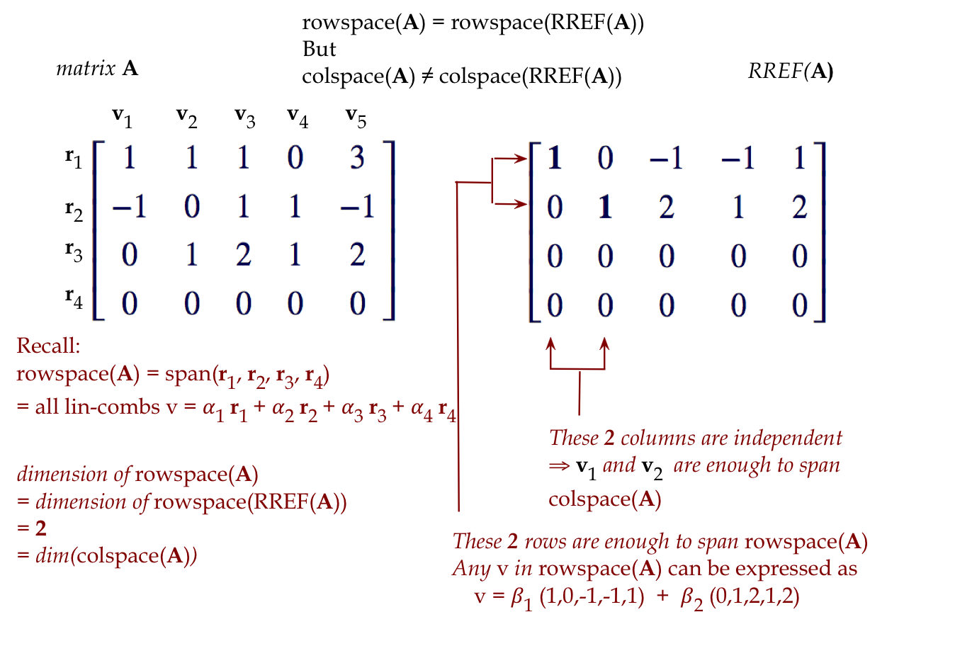
A few definitions as background
The following terms and notions will be needed, some
of which we've seen before.
- Let \({\bf A}_{m\times n}\) be a real matrix with rows
$$
\mat{
\ldots & {\bf r}_1 & \ldots\\
\ldots & {\bf r}_2 & \ldots\\
& \vdots & \\
\ldots & {\bf r}_m & \ldots\\
}
$$
and columns
$$
\mat{
& & & \\
\vdots & \vdots & & \vdots \\
{\bf c}_1 & {\bf c}_2 & \ldots & {\bf c}_n\\
\vdots & \vdots & & \vdots \\
& & &
}
$$
- Definition: The rowspace is the span of the
rows (treating the rows as vectors):
$$
\mbox{rowspace}({\bf A}) \eql
\mbox{span}({\bf r}_1, {\bf r}_2, \ldots, {\bf r}_m)
$$
- Definition: The colspace is the span of the
columns (treating the columns as vectors):
$$
\mbox{colspace}({\bf A}) \eql
\mbox{span}({\bf c}_1, {\bf c}_2, \ldots, {\bf c}_n)
$$
- Definition: The rank is the dimension of the
rowspace or the colspace (which we know are the same):
$$
\mbox{rank}({\bf A}) \eql
\mbox{dim}(\;\mbox{colspace}({\bf A})\; )
$$
- Definition: The nullspace is the set of all
vectors that solve \({\bf Ax}={\bf 0}\)
$$
\mbox{nullspace}({\bf A}) \eql
\{{\bf x}: {\bf Ax}={\bf 0} \}
$$
A useful picture to help recall the definitions and their meanings:
8.2
The theorem on invertibility and \({\bf Ax}={\bf b}\)
We've seen the first one before, but let's restate it in full
glory.
Theorem 8.1:
The following are equivalent (each
implies any of the others) for a real matrix \({\bf A}_{n\times n}\):
- \({\bf A}\) is invertible (the inverse exists).
- \({\bf A}^T\) is invertible.
- \(RREF({\bf A}) \eql {\bf I}\)
- \(\mbox{rank}({\bf A}) = n\).
- The rows are linearly independent.
- The columns are linearly independent.
- \(\mbox{nullspace}({\bf A})=\{{\bf 0}\}\)
\(\rhd\)
\({\bf Ax}={\bf 0}\) has \({\bf x}={\bf 0}\) as the only solution.
- \({\bf Ax}={\bf b}\) has a unique solution.
- \(\mbox{colspace}({\bf A})=\mbox{rowspace}({\bf A})=\mathbb{R}^n\)
Note:
- We saw most of this in the proofs relating to the RREF (Module 5)
and the results following the definition of linear independence
(Module 6).
- All of the proofs essentially boil down to understanding
what happens with the RREF.
8.3
The rank-nullity theorem
Theorem 8.2:
For a real matrix \({\bf A}_{m\times n}\),
\(
\mbox{rank}({\bf A}) + \mbox{dim}(\mbox{nullspace}({\bf A})) \eql n
\)
Intepretation and proof:
- Here, \(n\) = the number of columns.
- Recall: \(\mbox{nullspace}({\bf A}) =
\{{\bf x}: {\bf Ax}={\bf 0} \}\)
- That is, the set of all vectors \({\bf x}\) that satisfy
\({\bf Ax}={\bf 0}\).
- We first need to understand how the nullspace can have
a dimension.
- If a few linearly independent vectors within the nullspace
span the nullspace, then those vectors form a basis
for the nullspace.
- The number of such linearly independent vectors
is the dimension of the nullspace.
- The theorem says that the rank of the matrix and this
dimension are related.
- Paradoxically, this will be easier to
understand after the proof.
- But the proof itself will be easier to understand once
we look at an example.
- Consider the matrix
$$
{\bf A} \eql
\mat{
2 & 1 & 3 & 0 & 3\\
1 & 0 & 1 & 1 & 2\\
3 & 2 & 5 & -1 & 4\\
}
$$
- In solving \({\bf Ax}={\bf 0}\), we get the RREF
$$
\left[
\begin{array}{ccccc|c}
{\bf 1} & 0 & 1 & 1 & 2 & 0\\
0 & {\bf 1} & 1 & -2 & -1 & 0\\
0 & 0 & 0 & 0 & 0 & 0\\
\end{array}
\right]
$$
In-Class Exercise 2:
Use the RREF to write down the corresponding equations with
the basic variables on the left and free variables on the right.
Express \(x_1\) as a linear combination of \(x_3,x_4,x_5\).
Then express \(x_2\) as a linear combination of \(x_3,x_4,x_5\).
What are the solutions when:
- \(x_3=1,x_4=0,x_5=0\)?
- \(x_3=0,x_4=1,x_5=0\)?
- \(x_3=0,x_4=0,x_5=1\)?
- Clearly, any setting of values to the three free
variables will result in fixing the values of the basic variables.
- In particular consider the vectors
$$
{\bf v}_1 \eql \mat{-1 \\ -1\\ 1\\ 0\\ 0}
\;\;\;\;\;\;
{\bf v}_2 \eql \mat{-1 \\ 2\\ 0\\ 1\\ 0}
\;\;\;\;\;\;
{\bf v}_3 \eql \mat{-2 \\ 1\\ 0\\ 0\\ 1}
$$
Note:
- We want to argue that these three vectors span
the space of all possible solutions to \({\bf Ax}={\bf 0}\).
- Consider any solution \({\bf y}\) to \({\bf Ax}={\bf 0}\).
- Then, the 3D vector \((y_3, y_4, y_5)\)
can be expressed as a linear combination of
\((1,0,0), (0,1,0), (0,0,1)\), i.e.
$$
\vecthree{y_3}{y_4}{y_5}
\eql
\alpha
\vecthree{1}{0}{0}
+ \beta
\vecthree{0}{1}{0}
+ \gamma
\vecthree{0}{0}{1}
$$
for some choice of \(\alpha, \beta, \gamma\).
- But notice that
$$\eqb{
y_1 & \eql & (-1)\cdot y_3 + (-1)\cdot y_4 + (-2)\cdot y_5
& \;\;\;\;\;\;
\eql \mbox{ a linear combination of } y_3,y_4,y_5\\
y_2 & \eql & (-1)\cdot y_3 + (2) \cdot y_4 + (1)\cdot y_5
& \;\;\;\;\;\;
\eql \mbox{ a linear combination of } y_3,y_4,y_5
}$$
- Thus,
$$
\mat{y_1\\ y_2\\ y_3\\ y_4\\ y_5}
\eql
\alpha
\mat{-y_3-y_4-2y_5\\ -y_3 + 2y_4 + y_5\\ 1 \\ 0 \\ 0}
+ \beta
\mat{-y_3-y_4-2y_5\\ -y_3 + 2y_4 + y_5\\ 0 \\ 1 \\ 0}
+ \gamma
\mat{-y_3-y_4-2y_5\\ -y_3 + 2y_4 + y_5\\ 0 \\ 0 \\ 1}
$$
- What is the intuition here?
- The basic variable \(y_1\) is determined by whatever
choice of values we make for free variables \(y_3,y_4,y_5\).
- The form of this determination is a
linear combination.
- For example, we saw that
$$
y_1 \eql (-1)\cdot y_3 + (-1)\cdot y_4 + (-2)\cdot y_5
$$
- Thus, any linear combination of \(y_3,y_4,y_5\)
will determine \(y_1,y_2\) such that
\({\bf Ay}={\bf 0}\).
- Which means the dimension of this subspace of solutions
to \({\bf Ay}={\bf 0}\) is the number of
vectors needed to span all possible \(y_3,y_4,y_5\).
- In other words, the dimension is 3 (the number of free variables).
- Thus, the dimension of the nullspace is the same as
the number of non-pivot columns.
- Proof of Theorem 8.2:
Consider the RREF of \({\bf A}\). As we saw in Module 5, the pivot
columns determine the basic variables, which is the same
as the rank. As the argument above shows, the dimension of the
null space is exactly the number of non-pivot columns. Both sum
to \(n\). \(\;\;\;\;\Box\)
8.4
The Fundamental Theorem of linear algebra
To understand The fundamental theorem, we'll first need to understand the
orthogonal complement of a subspace:
- Think about the following two subspaces in 3D:
- \({\bf W}_{xy}\) = all vectors in the (x,y)-plane.
- \({\bf W}_{z}\) = all vectors along the z-axis.
- Clearly, every vector \({\bf u}\in {\bf W}_{xy}\) is
perpendicular to every vector \({\bf v}\in {\bf W}_{z}\).
- More importantly, if \({\bf v}\) is any vector that
is orthogonal to every \({\bf u}\in {\bf W}_{xy}\), then
\({\bf v}\in {\bf W}_{z}\).
- Thus, \({\bf W}_{z}\) contains all vectors that are
orthogonal to some vector in \({\bf W}_{xy}\).
\(\rhd\)
We say that \({\bf W}_{z}\) is the orthogonal complement
of \({\bf W}_{xy}\).
- For our 3D example, the statements above are obvious and
don't need proof.
- But in general, we will define orthogonal complement
as follows.
- Definition:
A vector \({\bf v}\) is orthogonal to a subspace \({\bf W}\)
if it is orthogonal to every vector in \({\bf W}\).
- Definition:
The orthogonal complement of a subspace \({\bf W}\), denoted
by \({\bf W}^\perp\), is the set of all vectors orthogonal to
\({\bf W}\).
- Clearly, \({\bf W} = ({\bf W}^\perp)^\perp\).
Theorem 8.3: (The fundamental theorem of linear algebra)
Let \({\bf A}_{m\times n}\) be a matrix with rank \(r\).
- \(\mbox{dim}(\mbox{colspace}({\bf A})) \eql r\)
- \(\mbox{dim}(\mbox{rowspace}({\bf A})) \eql r\)
- \(\mbox{dim}(\mbox{nullspace}({\bf A})) \eql n-r\)
- \(\mbox{dim}(\mbox{nullspace}({\bf A}^T)) \eql m-r\)
- \((\mbox{rowspace}({\bf A}))^\perp \eql \mbox{nullspace}({\bf A})\)
- \((\mbox{colspace}({\bf A}))^\perp \eql \mbox{nullspace}({\bf A}^T)\)
Interpretation and proof:
- We've already proved items 1-3:
- Parts 1-2 are Theorem 6.6.
- Part 3 follows directly from Theorem 8.2.
- Part 4 follows from applying 8.2 to the transpose.
- So, all that's new is Part 5 (because Part 6 is the same
thing applied to the transpose).
- Let's understand what it's saying:
- Every vector that's perpendicular to the row space is
in the nullspace (and vice-versa).
- The proof of Part 5 is surprisingly simple.
- Proof of Theorem 8.3:
We've already proved parts 1-4. For Part 5, let \({\bf x}\) be
any vector that is perpendicular to the row space. Then, the
dot product with every row is zero, which means \({\bf Ax}={\bf 0}\).
To go the other way, if \({\bf x}\) satisfies \({\bf Ax}={\bf 0}\),
that is, \({\bf x}\in \mbox{nullspace}({\bf A})\), then
the dot product with every row is zero, which means the dot
product with any linear combination of rows is also zero.
Thus, the dot product with any vector in the row space is zero,
or \({\bf x}\) is orthogonal to the row space.
\(\;\;\;\;\Box\)
We will explore two implications of Theorem 8.3
- A high-level conceptual one.
- Theorem 7.2, whose proof we postponed in Module 7
because we needed Theorem 8.3.
Recall:
Theorem 7.2: If the columns of \({\bf A}_{m\times n}\)
are linearly independent, then \(({\bf A}^T {\bf A})^{-1}\) exists.
First, the conceptual one:
- We'll start with a small result that will be needed.
- Proposition 8.4:
If \({\bf W}\) is a subspace of \(\mathbb{R}^n\) and
\({\bf x}\in \mathbb{R}^n\) then \({\bf x}\) can be
expressed uniquely as \({\bf x}={\bf y}+{\bf z}\) where
\({\bf y}\in{\bf W}\) and \({\bf z}\in{\bf W}^\perp\)
In-Class Exercise 3:
Before we get to the proof, draw an example in 3D with
\({\bf W}\) = the (x,y)-plane.
- We will do the proof in steps.
- Proof: (Step 1)
We need to show both that there exist such vectors
\({\bf x}\) and \({\bf y}\) and that they are unique.
Suppose \(\mbox{dim}({\bf W})=r\). Let
\({\bf v}_1, {\bf v}_2,\ldots,{\bf v}_r\) be a basis
for \({\bf W}\) and
\({\bf v}_{r+1}, {\bf v}_{r+2},\ldots,{\bf v}_n\)
be a basis for \({\bf W}^\perp\).
In-Class Exercise 4:
How do we know that \({\bf W}^\perp\) has
dimension \(n-r\)?
(Step 2)
Suppose
$$
\alpha_1{\bf v}_{1} + \alpha_2{\bf v}_{2} + \ldots +
\alpha_r{\bf v}_{r} + \alpha_{r+1}{\bf v}_{r+1} +
\alpha_{r+2}{\bf v}_{r+2} + \ldots +
\alpha_n{\bf v}_{n} \eql {\bf 0}
$$
We need to show that this implies all the \(\alpha_i\)'s are zero.
Define
$$\eqb{
{\bf y} & \eql & \alpha_1{\bf v}_{1} + \alpha_2{\bf v}_{2} + \ldots +
\alpha_r{\bf v}_{r}\\
{\bf z} & \eql & \alpha_{r+1}{\bf v}_{r+1} +
\alpha_{r+2}{\bf v}_{r+2} + \ldots +
\alpha_n{\bf v}_{n}
}$$
Then \({\bf y} + {\bf z} = {\bf 0}\) and thus
\({\bf y} = -{\bf z}\), which means \({\bf z}\) is
a scalar multiple of \({\bf y}\) and therefore in
the same subspace. But \({\bf y}\in {\bf W}\) because
it's a linear combination of \({\bf W}\)'s basis vectors and
similarly \({\bf z}\in {\bf W}^\perp\). The only way
this can happen is if
$$
{\bf y},{\bf z}\in {\bf W}\cap{\bf W}^\perp=\{{\bf 0}\}
$$
Since \({\bf v}_1, {\bf v}_2,\ldots,{\bf v}_r\) is a basis
for \({\bf W}\)
$$
\alpha_1{\bf v}_1 + \alpha_2{\bf v}_2 + \ldots
\alpha_r{\bf v}_r \eql {\bf 0}
\;\;\;\;\;\;\;\;
\Rightarrow \alpha_1=\alpha_2=\ldots\alpha_r=0
$$
Similarly,
$$
\alpha_{r+1}{\bf v}_{r+1} + \alpha_{r+2}{\bf v}_{r+2} + \ldots
\alpha_n{\bf v}_n \eql {\bf 0}
\;\;\;\;\;\;\;\;
\Rightarrow \alpha_{r+1}=\alpha_{r+2}=\ldots\alpha_n=0
$$
Therefore, all the \(\alpha_i\)'s are zero.
(Step 3) We've shown that \({\bf v}_1, {\bf v}_2,\ldots,{\bf v}_n\)
are linearly independent. Since the dimension of \(\mathbb{R}^n\)
is \(n\), then \({\bf v}_1, {\bf v}_2,\ldots,{\bf v}_n\) is
a basis for \(\mathbb{R}^n\). This means that any
\({\bf x}\in \mathbb{R}^n\) can be expressed as the
sum \({\bf x}={\bf y}+{\bf z}\) above with
\({\bf y}\in {\bf W}\) and \({\bf z}\in {\bf W}^\perp\).
(Step 4) We still need to show uniqueness. After all, could
different choices of bases for the subspaces result in a different sum?
Assume that \({\bf x}={\bf y}^\prime+{\bf z}^\prime\). Then, because
\({\bf x}={\bf y}+{\bf z}\), we equate and see that
\({\bf y}-{\bf y}^\prime={\bf z}-{\bf z}^\prime\), and therefore
both are in the same space.
But \({\bf y}-{\bf y}^\prime \in {\bf W}\) and
\({\bf z}-{\bf z}^\prime \in {\bf W}^\perp\) by assumption.
The only way this can happen is if
\({\bf y}-{\bf y}^\prime={\bf 0} = {\bf z}-{\bf z}^\prime\)
or \({\bf y}={\bf y}^\prime\) and \({\bf z}={\bf z}^\prime\).
\(\;\;\;\;\Box\)
- Whew! That was quite a long proof.
- We still haven't gotten around to our high-level conceptual
idea yet.
- Consider \({\bf Ax}={\bf b}\) where \({\bf A}_{m\times n}\) has
rank \(r\).
- Let \({\bf W}=\mbox{rowspace}({\bf A})\).
Now, Theorem 8.3 tells us that
\({\bf W}^\perp=\mbox{nullspace}({\bf A})\).
- Proposition 8.4 says that any \({\bf x}\in\mathbb{R}^n\)
can be written
uniquely as \({\bf x}={\bf y} + {\bf z}\) where
$$\eqb{
{\bf y} & \in & \mbox{rowspace}({\bf A})\\
{\bf z} & \in & \mbox{nullspace}({\bf A})\\
}$$
- Then,
$$\eqb{
{\bf b} & \eql & {\bf Ax} \\
& \eql & {\bf A}({\bf y} + {\bf z}) \\
& \eql & {\bf Ay} + {\bf Az} \\
& \eql & {\bf Ay} \\
}$$
In-Class Exercise 5:
Why is \({\bf Az}={\bf 0}\)?
- Now stare at
$$\eqb{
{\bf b} & \eql & {\bf Ax} \\
& \eql & {\bf Ay} \\
}$$
for a moment.
- Now for the important high-level observation:
- We started with \({\bf b} = {\bf Ax}\) where
\({\bf x}\in\mathbb{R}^n\) is any vector.
- Then we showed that \({\bf b} = {\bf Ay}\)
where \({\bf y}\) is a unique vector in the rowspace
corresponding to \({\bf x}\).
- Yet \({\bf b}\) is in the column space.
- This means that every matrix implies a unique mapping
of every vector in its rowspace to a vector in its column space.
- Another way of saying the same thing:
- Take any vector \({\bf b}\) in the column space.
- There is a unique vector \({\bf y}\) in the rowspace such
that \({\bf Ay}={\bf b}\).
- Thus, simple matrix-vector multiplication
provides a 1-1 mapping between its rowspace
and its column space.
- This is far from obvious and quite unexpected.
\(\rhd\)
Merely glancing through the proofs up to this point should
convince you that it's not obvious.
Finally, let's get to the proof of Theorem 7.2, which we
left pending from Module 7:
- Theorem 7.2: If the columns of \({\bf A}_{m\times n}\)
are linearly independent, then \(({\bf A}^T {\bf A})^{-1}\) exists.
- As a first step, let's prove the following.
- Proposition 8.5:
$$
\mbox{nullspace}({\bf A}) \eql \mbox{nullspace}({\bf A}^T {\bf
A})
$$
Proof:
Consider the solution to
$$
({\bf A}^T {\bf A}){\bf x}={\bf 0}
$$
We'll first write this as
$$
{\bf A}^T ({\bf A}{\bf x})={\bf 0}
$$
Which, if we define \({\bf y}={\bf A}{\bf x}\), means that
\({\bf A}^T{\bf y}={\bf 0}\) and therefore
$$
{\bf y}\in\mbox{nullspace}({\bf A}^T).
$$
Now \({\bf y}={\bf A}{\bf x}\), which means that
$$
{\bf y}\in\mbox{colspace}({\bf A}).
$$
Theorem 8.3 then implies that
$$
{\bf y}\in\mbox{nullspace}({\bf A}^T)^\perp
$$
So,
$$
{\bf y}\in\mbox{nullspace}({\bf A}^T)^\perp \cap
\mbox{nullspace}({\bf A}^T) \eql \{{\bf 0}\}.
$$
Which means \({\bf A}{\bf x}={\bf 0}\).
\(\;\;\;\;\Box\)
- Now we will complete the proof of 7.2
- Proof of Theorem 7.2:
Since we've assumed that \({\bf A}\) has full column rank
(columns are all linearly independent),
the only solution \({\bf A}{\bf x}={\bf 0}\) is
\({\bf x}={\bf 0}\). Proposition 8.5 showed that
setting \(({\bf A}^T {\bf A}){\bf x}={\bf 0}\) implied
\({\bf x}={\bf 0}\).
From Theorem 8.1, this means \(({\bf A}^T {\bf A})^{-1}\) exists.
\(\;\;\;\;\Box\)
A related useful result:
Lastly, let's use Theorem 8.3 to point out something that
seems obvious but needs proof:
- The set of all real-valued n-component vectors is called
\(\mathbb{R}^n\), pronounced as "R n".
- For example, \(\mathbb{R}^3\) is the set of
all 3D vectors \((x_1, x_2, x_3)\).
- Clearly, we know that \(n\) vectors are sufficient to
form a basis for \(\mathbb{R}^n\) because we can use the
\(n\) standard basis vectors.
- In 3D that would be:
$$
\vecthree{x_1}{x_2}{x_3}
\eql
x_1 \vecthree{1}{0}{0}
+
x_2 \vecthree{0}{1}{0}
+
x_3 \vecthree{0}{0}{1}
$$
- One could ask: can we do with fewer than \(n\)
vectors for a basis?
- Theorem 8.3 says "no":
- If it were possible, say with \(m \lt n\) basis vectors then
we could put these as rows into a matrix \({\bf A}_{m,n}\) where
the RREF would have at most \(m\) pivot rows.
- Then, Theorem 8.3 says the nullspace will have dimension
\(n-m\), which at least means it's non-empty.
- These nullspace vectors are orthogonal to the rowspace
vectors (and thus its basis).
- Which means the nullspace vectors can't be reached by
linear combination of the basis.
- To summarize, \(\mathbb{R}^n\) needs exactly \(n\)
vectors for a basis.
- Of course, a non-standard non-orthogonal basis could be used
but it would have to have \(n\) vectors.
8.5
An important fundamental theorem: the singular
value decomposition (SVD)
The SVD is easily one of the most useful results in linear algebra,
and a candidate for "The Second Fundamental Theorem of Linear Algebra".
First, let's state it and then explore.
Theorem 8.7:
Any real matrix \({\bf A}_{m\times n}\) with rank \(r\)
can be written as the product
$$
{\bf A} \eql
{\bf U}
{\bf \Sigma}
{\bf V}^T
$$
where \({\bf U}_{m\times m}\) and \({\bf V}_{n\times n}\) are real orthogonal matrices and
\({\bf \Sigma}_{m\times n}\) is a real diagonal matrix of the form
$$
{\bf \Sigma} \eql
\mat{
\sigma_1 & 0 & 0 & \ldots & & & 0\\
0 & \sigma_2 & 0 & \ldots & & & 0\\
\vdots & \vdots & \ddots & & & & 0\\
0 & 0 & \ldots & \sigma_r & & \ldots & 0\\
0 & \ldots & & & 0 & \ldots & 0 \\
0 & \ldots & & & \ldots & \ddots & 0\\
0 & \ldots & & & & \ldots & 0\\
}
$$
Let's start by exploring the middle matrix \({\bf \Sigma}\):
Next, let's explore \({\bf U}\) and \({\bf V}\):
- Recall from Theorem 7.4 (about orthogonal matrices)
- Multiplying a vector by an orthogonal matrix
does not change its length.
- An orthogonal matrix is equivalent to a series of reflections
or rotations.
- As we did in Module 4, we will
generate a series of \(N\) equally-spaced (by angle) vectors for
various angles \(\theta \in [0,2\pi]\).
- For example, with \(N=8\):
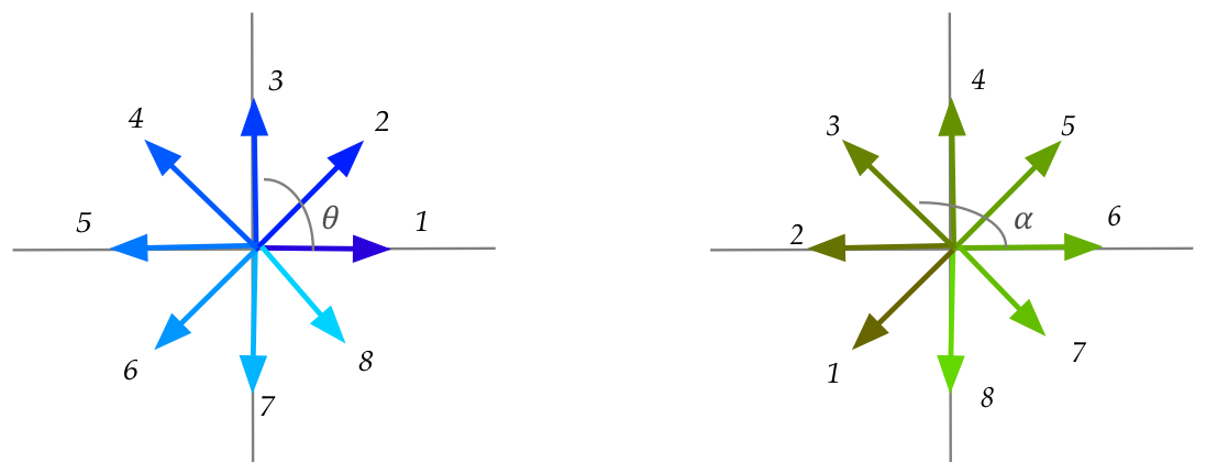
- The blue vectors on the left are generated in increments of
\(\frac{2\pi}{8}\).
- Let \(\theta_i\) be the angle of the i-th vector.
- Each blue vector is multiplied by an orthogonal matrix to produce
a corresponding green vector.
- The lengths are unchanged.
- Let \(\alpha_i\) be the angle of the i-th resulting vector.
- (All angles are measured from the rightward x-axis).
In-Class Exercise 9:
Draw a graph of \(\alpha_i\) vs. \(\theta_i\) for the above example.
In-Class Exercise 10:
Download SVDExplore.java
and compare the effect of transformation by
a random \({\bf A}\) and then its \({\bf U}\) and \({\bf V}\)
matrices when \({\bf A}={\bf U\Sigma V}^T\). In all three
cases, a graph of \(\alpha_i\) vs. \(\theta_i\) is plotted.
Execute a few different times for each case: each execution
creates a new random matrix.
You will also need lintool,
UniformRandom.java,
Function.java,
and SimplePlotPanel.java.
- Thus, we see that:
- The graph is complicated and non-linear for \({\bf A}\).
- There is a clear linear or inverse-linear relationship
when the matrix is orthogonal.
About the SVD:
- The SVD is one of the most powerful and practically useful results in
all of linear algebra.
- For example, we will see that SVD will give us something
called the pseudoinverse:
- Recall: not every matrix has an inverse.
- However, every matrix \({\bf A}\)
will turn out to have a pseudoinverse \({\bf A}^+\).
- To solve \({\bf Ax}={\bf b}\) approximately, compute
\({\bf A}^+\) and set \({\bf x} = {\bf A}^+ {\bf b}\).
- We will later see how to do this.
- The SVD is useful in applications:
- Image-search and topic identification in text.
- Compression.
- Low-rank approximations for the movie-rating problem.
- The SVD is a reliable way to determine the approximate rank
of a matrix.
- The RREF for very large matrices can result in compounding
errors (from lots or row transformations).
In-Class Exercise 11:
Create a 3x3 matrix with rank=1.
Download SVDRank.java
and enter your matrix to confirm the rank.
Observe that the remainder of the code generates random
matrices to compute the average rank. Increase the
number of such matrices. What is the intuition for why
it's hard to generate a random 3x3 matrix with rank less than 3?
[Hint: think about the columns, their independence, and use
a geometric interpretation].
One interpretation of the SVD:
- Recall: every matrix has a SVD:
$$
{\bf A} \eql
{\bf U}
{\bf \Sigma}
{\bf V}^T
$$
where \({\bf U}, {\bf V}\) are orthogonal and \({\bf \Sigma}\) is
diagonal.
- This means any transformation \({\bf Ax}\) of a vector \({\bf x}\)
by a matrix \({\bf A}\) can be decomposed into a sequence of
three transformations:
- An "almost" rotation/reflection (multiplication by \({\bf V}^T\)).
- A scaling (multiplication by \({\bf \Sigma}\)).
- A second "almost" rotation/reflection (multiplication by \({\bf U}\)).
- This is quite unexpected: every matrix transformation
is just really just three basic transformations applied sequentially!
8.6
Linear transformations
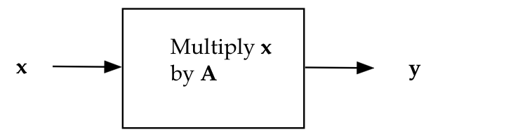
Consider what it means to transform a vector:
- So far, the only way we know is through multiplication by
a matrix.
- That is, we start with some vector \({\bf x}\), and multiply
by a matrix \({\bf A}\) to get a vector \({\bf y}\):
$$
{\bf y} \eql {\bf Ax}
$$
In-Class Exercise 12:
What is the relationship between the dimension of
\({\bf x}\) and the dimension of \({\bf y}\)?
- We can think of this as a general transformation that takes
in a vector and produces a vector:
- Let's use the notation
\({\bf y} = T({\bf x})\) for general vector-to-vector transformations.
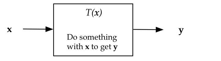
- We can imagine other ways of making a transformation.
In-Class Exercise 13:
Design a transformation, as weird as you would like,
that is obviously not related to matrix multiplication.
Linearity in transformations:
- Definition: A linear transformation \(T\) has
the property that for all vectors \({\bf x}, {\bf y}\) and
scalars \(\alpha, \beta\) the following is true:
$$
T(\alpha{\bf x} + \beta{\bf y}) \eql
\alpha T({\bf x}) + \beta T({\bf y})
$$
In-Class Exercise 14:
Is the transformation example you designed in an earlier exercise a
linear transformtion?
In-Class Exercise 15:
Show that:
- Matrix-vector multiplication \({\bf Ax}\) is a linear
transformation.
- If \(T\) is a linear transformation then
\(T({\bf 0}) = {\bf 0}\).
- Use the above result to show that a geometric
translation cannot be a linear transformation.
(Remember, in the second case, both the argument and result are
the zero vector).
And now for a fundamental, yet surprisingly easy to prove result:
- Theorem 8.9:
For every linear transformation \(T\) there is an equivalent matrix
\({\bf A}\) such that \(T({\bf x}) = {\bf Ax}\) for all \({\bf x}\).
- Before proving, let's understand what it's saying:
- In essence, a linear transformation can only be a matrix
multiplication, nothing else.
- Even if a linear transformation looks very not-matrix-like,
it is equivalent to a matrix.
- Proof of Theorem 8.9: Let's do this in steps.
Suppose the transformation \(T\) maps n-dimensional vectors into
m-dimensional vectors.
- Consider the n standard vectors of dimension n:
\({\bf e}_1, {\bf e}_2, \ldots, {\bf e}_n\).
In-Class Exercise 16:
What are the standard vectors for \(n=4\)?
- Define the vectors
$$
{\bf c}_1 \eql T({\bf e}_1),
\;\;\;\;\;\;
{\bf c}_2 \eql T({\bf e}_2),
\;\;\;\;\;\;
\ldots,
\;\;\;\;\;\;
{\bf c}_n \eql T({\bf e}_n),
$$
In-Class Exercise 17:
What is the dimension of each \(T({\bf e}_i)\)?
- Put the \(n\) \({\bf c}_i\)'s as columns of a matrix \({\bf A}\).
- Any vector \({\bf x}=(x_1,x_2,\ldots,x_n)\) can
be written as
$$
x_1 {\bf e}_1 + x_2 {\bf e}_2 + \ldots + x_n {\bf e}_n
$$
In-Class Exercise 18:
Why is this true? Give an example with \(n=4\).
- Now apply the transformation \(T\):
$$\eqb{
T({\bf x})
& \eql &
T(x_1 {\bf e}_1 + x_2 {\bf e}_2 + \ldots + x_n {\bf e}_n) \\
& \eql &
x_1 T({\bf e}_1) + x_2 T({\bf e}_2) + \ldots + x_n T({\bf e}_n)\\
& \eql &
x_1 {\bf c}_1 + x_2 {\bf c}_2 + \ldots + x_n {\bf c}_n\\
}$$
In-Class Exercise 19:
The third step is from the definition of the
\({\bf c}_i\)'s but what let's us conclude the second step from
the first?
- Finally, the last step above is a linear combination of the
columns of \({\bf A}\) using the elements of \({\bf
x}\).
- In other words:
$$
x_1 {\bf c}_1 + x_2 {\bf c}_2 + \ldots + x_n {\bf c}_n
\eql {\bf Ax}
$$
- And so, \(T({\bf x}) = {\bf Ax}\).
\(\;\;\;\;\;\Box\)
An interpretation of Theorem 8.9:
- Imposing linearity on a transformation is actually quite
restrictive.
- To see why, let's go back to the step where
$$\eqb{
T({\bf x})
& \eql &
T(x_1 {\bf e}_1 + x_2 {\bf e}_2 + \ldots + x_n {\bf e}_n) \\
& \eql &
x_1 T({\bf e}_1) + x_2 T({\bf e}_2) + \ldots + x_n T({\bf e}_n)\\
}$$
- Once a linear transformation has taken a linear combination
of the standard vectors, it is forced to produce the
same linear combination of the transformed standard vectors.
- Thus, a linear transformations actions on standard vectors
completely determine its action on any vector.
- It so happens, of course, that a linear combination of
vectors is written as a matrix-vector product
\(\rhd\)
This is how matrices were defined
- Thus, it is now perhaps not so surprising that linear
transformations and matrix-vector multiplications are the same thing.
8.7
Highlights and study tips
Highlights:
- The purpose of this module was to give you a high-level
overview of some of the major theoretical results in linear algebra.
- When \({\bf Ax}={\bf b}\) has a solution, many things are
simultaneously implied:
- \({\bf A}\) has an inverse.
- \({\bf A}\)'s rows and columns are linearly independent.
- The solution is unique.
- There are two obvious spaces related to a matrix
\({\bf A}\):
- Row space: the span of its rows.
- Column space: the span of its columns.
- The less apparent ones are the the nullspace and the
nullspace of the transpose.
- The Fundamental Theorem of Linear Algebra finds two
different relationships between these spaces:
- In terms of dimension: for example, the sum of
dimensions of the rowspace and nullspace is the number of columns.
- In terms of orthogonality: the rowspace and
nullspace are orthogonal complements.
- The orthogonality of spaces is useful in some proofs.
- The SVD should really be a called Second Fundamental Theorem of
Linear Algebra.
- The SVD's internals and uses are still to be described
(later modules).
- A linear transformation and a matrix are one and the same thing.
Study tips:
- The most important thing to learn in this module is how to
read and interpret the theorems.
- In general, in the future, learning to
understand what a result is saying is much more important
than learning to reproduce the proof.
- Start by breaking a theorem down into pieces. Are the pieces
understandable on their own?
- Create an example to go hand-in-hand with understanding a
theorem, as we did with Theorem 8.2.