Module objectives
By the end of this module, you should be able to
- Describe and implement the least-squares solution to
\({\bf Ax}={\bf b}\).
- Describe and compute vector projections.
- Demonstrate through code the Gram-Schmidt algorithm for
finding an orthogonal basis.
- Explain the QR decomposition.
- List and explain properties of orthogonal matrices.
7.0
Things to recall
Let's review a few ideas that will be useful:
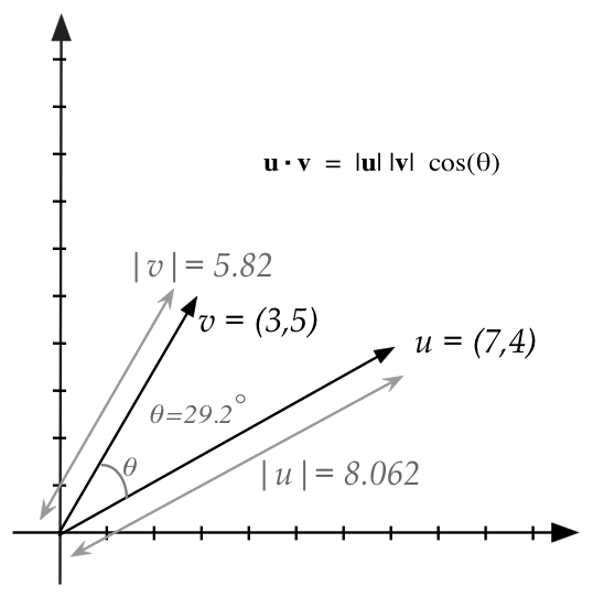
- Recall dot product:
- Example: \({\bf u} = (7,4)\) and \({\bf v} = (3,5)\)
$$
{\bf u} \cdot {\bf v} \eql (7,4) \cdot (3,5)
\eql 41
$$
- Vector length:
- Example: \({\bf u} = (7,4)\)
$$
|{\bf u}| \eql \sqrt{u_1^2 + u_2^2} \eql \sqrt{7^2 + 4^2} \eql 8.062
$$
- We can write this as
$$
|{\bf u}| \eql \sqrt{{\bf u} \cdot {\bf u}}
\eql \sqrt{(7,4)\cdot(7,4)} \;\;\;\;\;\;\mbox{ in the example above}
$$
- Relationship between dot-product and angle:
- For any two vectors:
$$
{\bf u} \cdot {\bf v}
\eql
|{\bf u}| |{\bf v}|
\cos(\theta)
$$
- Thus,
$$
\cos(\theta)
\eql
\frac{{\bf u} \cdot {\bf v}}{
|{\bf u}| |{\bf v}|}
$$
- Example: \({\bf u} = (7,4)\) and \({\bf v} = (3,5)\)
$$
\cos(\theta)
\eql
\frac{{\bf u} \cdot {\bf v}}{
|{\bf u}| |{\bf v}|}
\eql
\frac{41}{8.062 \times 5.83}
\eql 0.8721
$$
- So, \(\theta = \cos^{-1}(0.8721) = 0.511\mbox{ radians } = 29.2^\circ\)
- In a figure:
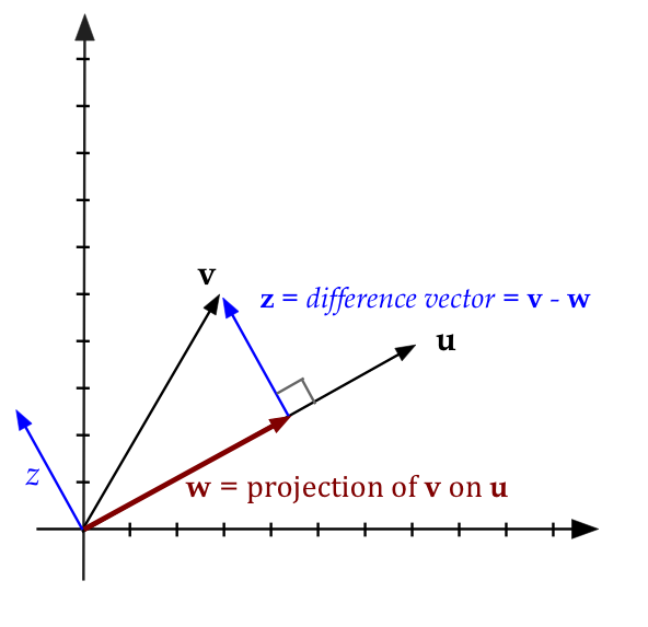
- The projection of one vector on another:
- Consider
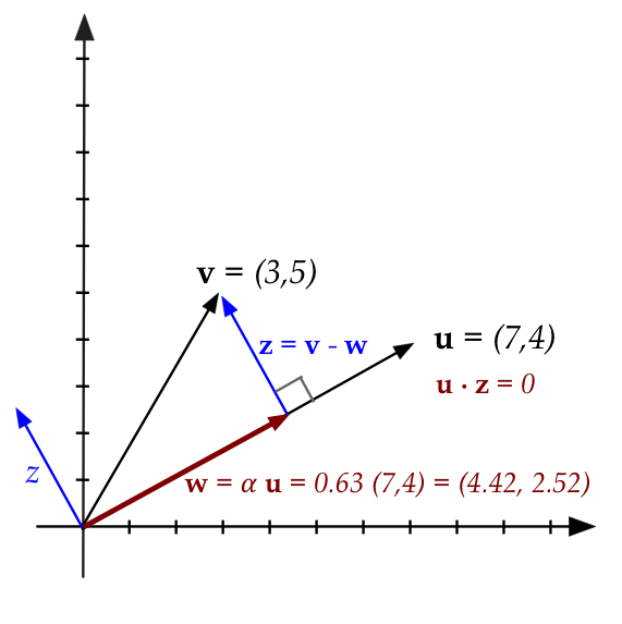
- Here, \({\bf w}\) is some stretch of \({\bf u}\)
$$
{\bf w} \eql \alpha {\bf u}
$$
- \({\bf z}\) is the difference vector with \({\bf v}\)
$$
{\bf z} \eql {\bf v} - {\bf w}
$$
- For some value of \(\alpha\)
\({\bf z}\) will be perpendicular to \({\bf u}\)
- This stretch we've shown in Module 4 is:
$$
\alpha \eql
\left(\frac{{\bf u}\cdot {\bf v}}{{\bf u}\cdot {\bf u}} \right)
$$
- The vector \({\bf w}\) is called the projection
of \({\bf v}\) on \({\bf u}\)
$$
{\bf w} \eql \mbox{proj}_{\bf u}({\bf v})
$$
- In the figure:
- The tranpose of a matrix:
- Example:
$$
{\bf A} \eql
\mat{6 & 4 & 8\\
2 & 3 & 1\\
0 & 0 & 0}
\;\;\;\;\;\;\;\;
{\bf A}^T \eql
\mat{6 & 2 & 0\\
4 & 3 & 0\\
8 & 1 & 0}
$$
- Thus, the i-th row of \({\bf A}^T\) is the i-th column of \({\bf A}\)
- One view of matrix-vector
multiplication: a linear combination of its columns:
$$
\mat{6 & 4 & 8\\
2 & 3 & 1\\
0 & 0 & 0}
\vecthree{x_1}{x_2}{x_3}
\eql
x_1 \vecthree{6}{2}{0}
+
x_2 \vecthree{4}{3}{0}
+
x_3 \vecthree{8}{1}{0}
$$
- Another view: dot products of the matrix's rows
$$
\mat{6 & 4 & 8\\
2 & 3 & 1\\
0 & 0 & 0}
\vecthree{x_1}{x_2}{x_3}
\eql
\mat{
\ldots & {\bf r}_1 & \ldots \\
\ldots & {\bf r}_2 & \ldots \\
\ldots & {\bf r}_3 & \ldots
}
{\bf x}
\eql
\mat{
{\bf r}_1 \cdot {\bf x} \\
{\bf r}_2 \cdot {\bf x} \\
{\bf r}_3 \cdot {\bf x}
}
$$
7.1
The problem with solving \({\bf Ax}={\bf b}\)
The difficulty with \({\bf Ax}={\bf b}\) is '\({\bf =}\)'
Consider the following \({\bf Ax}={\bf b}\) example:
$$
\mat{6 & 4 & 8\\
2 & 3 & 1\\
0 & 0 & 0}
\vecthree{x_1}{x_2}{x_3}
\eql
\vecthree{5}{6}{3}
$$
- Clearly, there is no solution.
- It might seem reasonable to expect no solution.
- However, the following also has no solution:
$$
\mat{6 & 4 & 8\\
2 & 3 & 1\\
0 & 0 & 0}
\vecthree{x_1}{x_2}{x_3}
\eql
\vecthree{5}{6}{0.001}
$$
while
$$
\mat{6 & 4 & 8\\
2 & 3 & 1\\
0 & 0 & 0}
\vecthree{x_1}{x_2}{x_3}
\eql
\vecthree{5}{6}{0}
$$
does have a solution \(x_1=-0.9, x_2=2.6, x_3=0\).
- The RREF approach only finds exact solutions.
\(\rhd\)
Even a tiny numerical error could result in a non-solution.
- What we really need: a way to find good approximate solutions.
Let's examine the geometry for some insight:
- Observe that if
$$
\mat{6 & 4 & 8\\
2 & 3 & 1\\
0 & 0 & 0}
\vecthree{x_1}{x_2}{x_3}
\eql
\vecthree{5}{6}{3}
$$
has no solution, this means that \({\bf b}=(5,6,3)\) is not in the
column space of \({\bf A}\).
\(\rhd\)
That is, no linear combination of the columns can give us
\({\bf b}\).
- Suppose we name the columns (column vectors)
\({\bf c}_1,{\bf c}_2, {\bf c}_3\).
In-Class Exercise 1:
Download EquationExample3D.java
and plot all three columns as vectors, and the
vector \({\bf b}=(5,6,3)\).
- Clearly, \({\bf b}\) does not lie in the span of the
columns \(\mbox{span}({\bf c}_1,{\bf c}_2,{\bf c}_3)\).
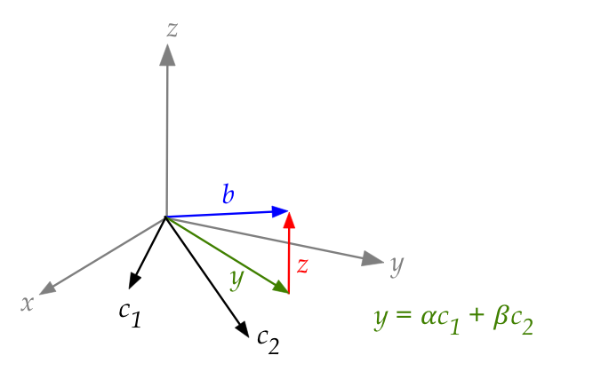
- We could then ask the question: which vector in the span
is closest to \({\bf b}\)?
In-Class Exercise 2:
Download SearchClosest3D.java
which tries various linear combinations \({\bf y}=\alpha{\bf c}_1 + \beta{\bf c}_2\)
to pick the one closest to \({\bf b}\).
- Why is \({\bf c}_3\) not included in the linear combination?
- Un-comment the code at the end to draw the vector from
\({\bf y}\) to \({\bf b}\).
- Draw by hand the three axes, vectors
\({\bf c}_1,{\bf c}_2, {\bf b}\) and your solution to the
closest \({\bf y}\).
- Change the range of search to see if you can get a closer \({\bf y}\).
Let's now explore an idea:
- Consider a point above a plane.
- Claim: the shortest distance from the point to the plane
is on the perpendicular to the plane.
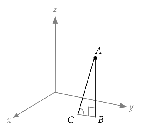
In-Class Exercise 3:
Prove that this is the case using the picture above.
- Now let's go back to the approximate solution for
$$
\mat{6 & 4 & 8\\
2 & 3 & 1\\
0 & 0 & 0}
\vecthree{x_1}{x_2}{x_3}
\eql
\vecthree{5}{6}{3}
$$
which we will write as
$$
\mat{\vdots & \vdots & \vdots\\
{\bf c}_1 & {\bf c}_2 & {\bf c}_3\\
\vdots & \vdots & \vdots}
\vecthree{\alpha}{\beta}{0}
\approx
{\bf b}
$$
- We'll write the LHS as
$$
\mat{\vdots & \vdots & \vdots\\
{\bf c}_1 & {\bf c}_2 & {\bf c}_3\\
\vdots & \vdots & \vdots}
\vecthree{\alpha}{\beta}{0}
\eql
{\bf y}
$$
where \({\bf y}\) is in the column space.
- Note: in this particular example, we've shown earlier
that we only need \({\bf c}_1\) and \({\bf
c}_2\) to form the linear combination
$$
{\bf y} \eql \alpha {\bf c}_1 + \beta {\bf c}_2
$$
- The goal: solve for \(\alpha, \beta\) to find the
closest \({\bf y}\) to \({\bf b}\).
- Let
$$
{\bf z} \defn {\bf b} - {\bf y}
$$
be the "error" or distance between the closest linear combination
\({\bf y}\) and \({\bf b}\):
In-Class Exercise 4:
Prove that \({\bf z}\) is orthogonal to
\({\bf c}_1\) and \({\bf c}_2\).
- We will now solve for \(\alpha, \beta\).
- First, since \({\bf y} = \alpha {\bf c}_1 + \beta {\bf c}_2\)
$$\eqb{
{\bf z} & \eql & {\bf b} - {\bf y} \\
& \eql & {\bf b} - \alpha {\bf c}_1 - \beta {\bf c}_2
}$$
- Next, since the vector \({\bf z}\) is orthogonal to
\({\bf c}_1\) and \({\bf c}_2\), the dot products below
must be zero:
$$\eqb{
{\bf c}_1 \cdot {\bf z} \eql 0 \\
{\bf c}_2 \cdot {\bf z} \eql 0 \\
}$$
In other words
$$\eqb{
{\bf c}_1 \cdot ({\bf b} - \alpha {\bf c}_1 - \beta {\bf c}_2) \eql 0 \\
{\bf c}_2 \cdot ({\bf b} - \alpha {\bf c}_1 - \beta {\bf c}_2) \eql 0 \\
}$$
Which gives us two equations for \(\alpha, \beta\).
In-Class Exercise 5:
Use the data in the example to above to write down the equations
for \(\alpha, \beta\). Then, solve the equations by hand or
by using the demo equation solver from Module 1.
After, enter the values of \(\alpha,\beta\) in
PlotClosest3D.java
to see both \({\bf y}\) and \({\bf z}\).
7.2
The Least-Squares Method
We will write the equations in matrix form:
The least squares algorithm:
- Recall our goal: to solve \({\bf Ax}={\bf b}\) approximately
when the RREF declares that \({\bf Ax}={\bf b}\) has no
exact solution.
- We know that the best approximate solution \(\hat{\bf x}\)
satifies
$$
{\bf A}^T ({\bf b} - {\bf A}\hat{\bf x}) \eql {\bf 0}
$$
- Interpretation:
- The term \({\bf A}\hat{\bf x}\) is the linear combination
that's closest to \({\bf b}\).
- \(({\bf b} - {\bf A}\hat{\bf x})\) is
the difference vector.
- The difference vector is orthogonal to each column of
\({\bf A}\).
- And therefore orthogonal to each row of \({\bf A}^T\).
- Which is what the equation is saying.
- Next, let's expand the expression
$$
{\bf A}^T {\bf b} - {\bf A}^T {\bf A}\hat{\bf x} \eql {\bf 0}
$$
Or
$$
{\bf A}^T {\bf A} \hat{\bf x}
\eql
{\bf A}^T {\bf b}
$$
Which we'll write as
$$
({\bf A}^T {\bf A}) \hat{\bf x}
\eql
{\bf A}^T {\bf b}
$$
- Finally, suppose the matrix \(({\bf A}^T {\bf A})\)
has an inverse \(({\bf A}^T {\bf A})^{-1}\).
- Then, multiplying both sides by this inverse:
$$
({\bf A}^T {\bf A})^{-1}
({\bf A}^T {\bf A}) \hat{\bf x}
\eql
({\bf A}^T {\bf A})^{-1}
{\bf A}^T {\bf b}
$$
- We now finally have a direct expression for the approximate
solution \(\hat{\bf x}\):
$$
\hat{\bf x}
\eql
({\bf A}^T {\bf A})^{-1}
{\bf A}^T {\bf b}
$$
(Provided of course the inverse exists).
- This is called the least-squares solution to \({\bf Ax}={\bf b}\).
- The method and terminology dates back to Gauss, who started
by minimizing \(({\bf Ax}-{\bf b})^2\).
\(\rhd\)
Which results in the same solution.
In-Class Exercise 8:
Why does this result in the same solution? That is, why
is our solution the solution to minimizing \(({\bf Ax}-{\bf b})^2\)?
(Hint: make a simple geometric argument)
- To see how significant this is, let's first do a "sanity
check" of the dimensions.
In-Class Exercise 9:
Suppose \({\bf A}_{m\times n}\) is a matrix with \(m\) rows
and \(n\) columns. What are the dimensions of \({\bf A}^T {\bf A}\)?
Verify that the dimensions all work out correctly
in the expression \(({\bf A}^T {\bf A})^{-1} {\bf A}^T {\bf b}\).
- Recall the earlier difficulties with solving \({\bf Ax}={\bf b}\):
- A unique solution exists only if both \({\bf A}\) is square,
and if \({\bf A}^{-1}\) exists.
- If \({\bf A}\) is not square, there typically is no
solution or multiple solutions exist.
(In rare cases, as we saw in Module 5, a non-square
matrix could result in a unique solution.)
- If there are too many equations (more rows than columns) it's
highly unlikely that a solution exists.
- Small numerical errors can result in a no-solution case.
- The least-squares solution neatly addresses all of these
issues:
- It applies to non-square matrices as well.
- The least-squares solution is unique.
\(\rhd\)
Because there's a unique closest vector to \({\bf b}\).
For least-squares to be truly useful, we'd have to address two questions
- If \({\bf A}\) is square and \({\bf Ax}={\bf b}\) does have
a solution \({\bf x}= {\bf A}^{-1}{\bf b}\), then
is that
solution the same as the least squares
solution \(\hat{\bf x} = ({\bf A}^T {\bf A})^{-1} {\bf A}^T {\bf b}\)?
- For any matrix \({\bf A}_{m\times n}\) how likely is it that
\(({\bf A}^T {\bf A})^{-1}\) exists?
Luckily:
- Theorem 7.1: If \({\bf A}^{-1}\) exists, then
\(({\bf A}^T {\bf A})^{-1} {\bf A}^T {\bf b} = {\bf A}^{-1}{\bf
b}\).
- This is good news: the least-squares solution is
the exact solution if the exact solution exists.
- Theorem 7.2: If the columns of \({\bf A}_{m\times n}\)
are linearly independent, then \(({\bf A}^T {\bf A})^{-1}\) exists.
- Let's understand what 7.2 is saying:
- If \(m < n\) then the column rank (which is the row rank)
is less than \(n\).
\(\rhd\)
The columns cannot be linearly independent.
- If \(m \geq n\) then it's possible that the columns are
independent.
\(\rhd\)
In which case, least-squares will work.
- Unfortunately, neither result is easy to prove. We'll need
to roll up our sleeves.
Let's start with the first result, which is the easier of the two:
- We will do this in steps.
- Suppose we could show that
$$
({\bf A}^T {\bf A})^{-1} \eql {\bf A}^{-1} ({\bf A}^T)^{-1}
$$
In-Class Exercise 10:
Use the above result to complete the proof of Theorem 7.1.
- Thus, what remains is to show that
$$
({\bf A}^T {\bf A})^{-1} \eql {\bf A}^{-1} ({\bf A}^T)^{-1}
$$
- We really need to show two things here:
- If \({\bf A}^{-1}\) exists, so does \(({\bf A}^T)^{-1}\).
- And that the inverse-transpose multiplication can be
switched as above.
In-Class Exercise 11:
If \({\bf A}^{-1}\) exists, what does this tell us about the
dimensions and column rank of \({\bf A}\)? And what does that tell us about the row
rank of \({\bf A}\), and therefore the column rank
of \({\bf A}^{T}\)? What can we conclude about whether
\(({\bf A}^T)^{-1}\) exists?
- Now consider any two matrices \({\bf A}\) and \({\bf B}\)
whose inverses exist.
- Consider the product \({\bf AB}\) and left multiply this
by the inverses in opposite order:
$$\eqb{
({\bf B}^{-1} {\bf A}^{-1}) {\bf A B}
& \eql &
{\bf B}^{-1} ({\bf A}^{-1} {\bf A}) {\bf B}\\
& \eql &
{\bf B}^{-1} ({\bf I}) {\bf B}\\
& \eql &
{\bf B}^{-1} ({\bf I} {\bf B})\\
& \eql &
{\bf B}^{-1} {\bf B}\\
& \eql &
{\bf I}
}$$
- Which means that
$$
({\bf A B})^{-1} \eql {\bf B}^{-1} {\bf A}^{-1}
$$
In-Class Exercise 12:
Use this to complete the proof of Theorem 7.1 and write out the whole
proof step by step.
The proof of 7.2 is more involved.
It will have to await the proof of an even more dramatic result
\(\rhd\)
The so-called fundamental theorem of linear algebra.
We will get to this later in Theory, Part II.
Let's now return to our running example and apply the least-squares
method:
- First consider the \({\bf Ax}={\bf b}\) example:
$$
\mat{6 & 4\\
2 & 3\\
0 & 0}
\vectwo{x_1}{x_2}
\eql
\vecthree{5}{6}{3}
$$
- The matrix \({\bf A}\) here consists of the two column
vectors
$$
{\bf c}_1 \eql \vecthree{6}{2}{0}
\;\;\;\;\;\;\;\;
\mbox{and}
\;\;\;\;\;\;\;\;
{\bf c}_2 \eql \vecthree{4}{3}{0}
$$
- Both are in the (x,y)-plane.
- Whereas \({\bf b}=(5,6,3)\) is not.
- Thus, no linear combination of the columns can give us \({\bf b}\).
- In other words the equation
$$
x_1 {\bf c}_1
+ x_2{\bf c}_2 \eql \vecthree{5}{6}{3}
$$
has no solution.
- That is, \({\bf Ax}={\bf b}\) has no exact solution.
- The two columns, however, are linearly independent (recall
the 3D drawing).
\(\rhd\)
Theorem 7.2 says that a least-squares solution is possible.
- Let's do this in steps with
- The transpose is
$$
{\bf A}^T \eql
\mat{6 & 2 & 0\\
4 & 3 & 0
}
$$
- The product \({\bf A}^T {\bf A}\) turns out to be
$$
{\bf A}^T {\bf A} \eql
\mat{40 & 30\\
30 & 25}
$$
- The inverse can be computed as
$$
({\bf A}^T {\bf A})^{-1} \eql
\mat{0.25 & -0.3\\
-0.3 & 0.4}
$$
- Finally, we compute the least squares solution
$$\eqb{
\hat{\bf x}
& \eql &
({\bf A}^T {\bf A})^{-1} {\bf A}^T {\bf b} \\
& \eql &
\mat{0.25 & -0.3\\
-0.3 & 0.4}
\mat{6 & 2 & 0\\
4 & 3 & 0}
\vecthree{5}{6}{3} \\
& \eql &
\vectwo{-0.9}{2.6}
}$$
In-Class Exercise 13:
Download LeastSquaresExample3D.java
to implement the above solution and confirm. You will
also need MatrixTool.class
(or your own MatrixTool.java).
Note: this will work only if lintool.jar is in your CLASSPATH.
In-Class Exercise 14:
Add the column \({\bf c}_3=(8,1,0)\) to the matrix \({\bf A}\)
in the above code.
- Explain why the columns are not linearly independent.
- What happens as a result?
7.3
Least squares application: linear regression
The (linear) regression problem:
- We'll consider the simplest form, with two variables.
- In this type of problem, we are given data
\((x_1,y_1), (x_2,y_2), (x_3,y_3), \ldots, (x_n,y_n)\).
- For example, here are \(n=8\) data points, with
potential measurement error:
| x |
y |
| 1 |
3.6 |
| 1.5 |
3.9 |
| 2 |
3.9 |
| 3.6 |
5.1 |
| 5.0 |
5.2 |
| 6.2 |
6.0 |
| 8.5 |
7.4 |
| 9.0 |
7.2 |
- We'd like to see if a line can approximately
explain the relationship between \(y\) and \(x\):
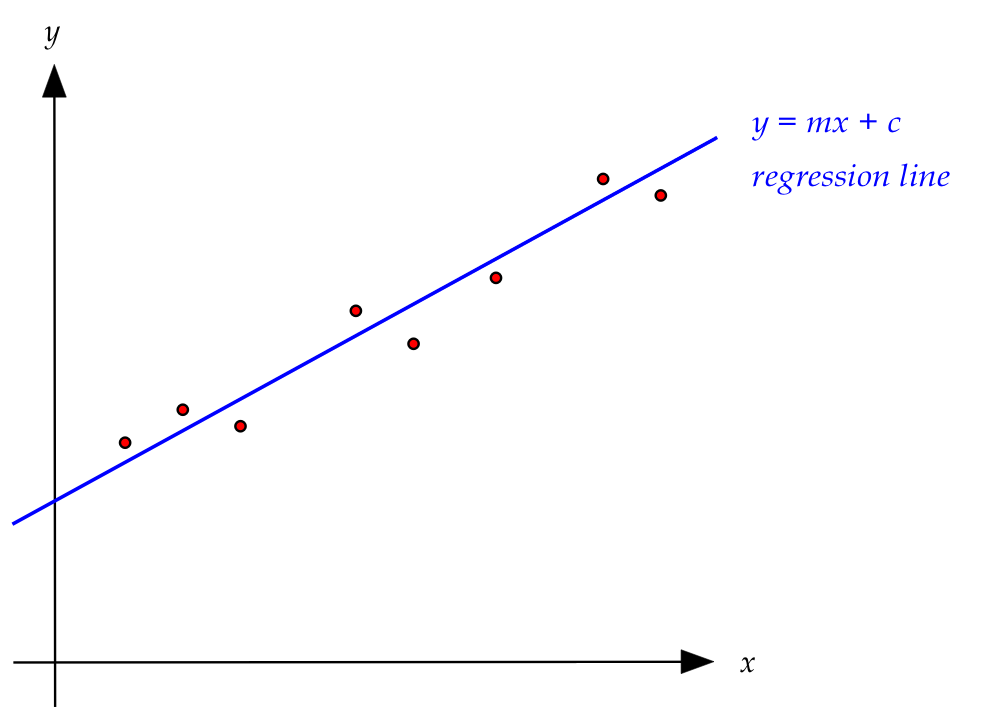
- In fact, we would like the best line that fits the
data.
- Suppose the equation of that line is \(y=mx + c\)
\(\rhd\)
That is, slope=\(m\) and y-intercept=\(c\).
- If a linear relationship existed and the data were perfect,
then for each data sample \((x_i,y_i)\) it would be true that
\(y_i = mx_i + c\).
- That is,
$$\eqb{
y_1 & \eql & mx_1 + c\\
y_2 & \eql & mx_2 + c\\
y_3 & \eql & mx_3 + c\\
\vdots & & \vdots \\
y_n & \eql & mx_n + c\\
}$$
which we will write as
$$\eqb{
x_1m + c & \eql & y_1 \\
x_2m + c & \eql & y_2 \\
x_3m + c & \eql & y_3 \\
\vdots & & \vdots \\
x_nm + c & \eql & y_n \\
}$$
- In matrix form:
$$
\mat{x_1 & 1\\
x_2 & 1\\
x_3 & 1\\
\vdots & \vdots\\
x_n & 1\\}
\vectwo{m}{c}
\eql
\mat{y_1\\ y_2 \\ y_3 \\ \vdots \\ y_n}
$$
- In our more familar notation of \({\bf Ax}={\bf b}\):
$$
{\bf A} \eql
\mat{x_1 & 1\\
x_2 & 1\\
x_3 & 1\\
\vdots & \vdots\\
x_n & 1\\}
\;\;\;\;\;\;\;\;\;\;
{\bf x} \eql
\vectwo{m}{c}
\;\;\;\;\;\;\;\;\;\;
{\bf b} \eql
\mat{y_1\\ y_2 \\ y_3 \\ \vdots \\ y_n}
$$
Note: the vector \({\bf x}\) and the data values \(x_i\) are
different things.
- Because the data has errors, an exact solution will be
impossible (too many equations).
- The least squares approximation is:
$$
\hat{\bf x}
\eql
({\bf A}^T {\bf A})^{-1} {\bf A}^T {\bf b}
$$
- Important: the "x" in the data has nothing to do with the "x"
in \(\hat{\bf x}\).
- Once we solve for \(\hat{\bf x}\), we will get
$$
\hat{\bf x} \eql \vectwo{\hat{m}}{\hat{c}}
$$
That is, an approximation for the two parameters
\(m\) and \(c\).
In-Class Exercise 15:
Download RegressionExample.java,
compile and execute to view the data. Then un-comment the
least-squares part of the code, add code to complete the least-squares
calculation. What are the values of \(\hat{m}\) and \(\hat{c}\)?
Fitting a plane:
- The same idea generalizes to any linear relationship between
variables of the kind
$$
a_1 x_1 + a_2 x_2 + \ldots + a_nx_n \eql \mbox{a constant}
$$
- For example, consider 3D points \((x_i,y_i,z_i)\) as data.
- Here, we want to find a plane \(ax + by + cz = d\)
that best fits the data.
- We'll divide by \(c\) and write the equation as:
$$
a^\prime x + b^\prime y - d^\prime = -z
$$
- Then, given the data,
$$
\mat{x_1 & y_1 & -1\\
x_2 & y_2 & -1\\
x_3 & y_3 & -1\\
\vdots & \vdots & \vdots\\
x_n & y_n & -1\\}
\mat{a^\prime \\ b^\prime \\ d^\prime}
\eql
\mat{-z_1 \\ -z_2 \\ -z_3 \\ \vdots \\ -z_n}
$$
Which we can solve using least squares.
In-Class Exercise 16:
Download RegressionExample3D.java,
compile and execute to view the data. Then un-comment the
least-squares part of the code, add code to complete the least-squares
calculation and plot a plane.
7.4
Least squares application: curve fitting
Let's examine how the least-squares approach can be used to
fit curves to data:
- We'll go back to Gauss' ellipse and find the best ellipse
to fit given data.
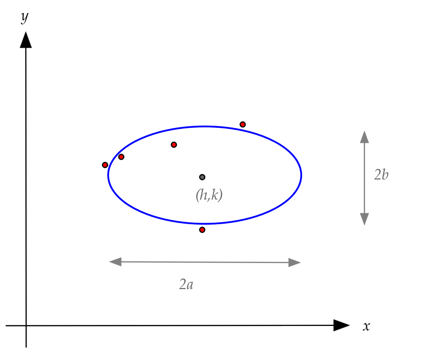
- We'll focus on an axis-parallel ellipse that's wider in the
x-direction.
- The equation for an ellipse centered at \((h,k)\) with
major axis \(2a\) and minor axis \(2b\) is
$$
\frac{(x-h)^2}{a^2} + \frac{(y-k)^2}{b^2} \eql 1
$$
- The data will consist of \(n\) points \((x_i,y_i)\).
- First, notice that the standard parameters \(h,k,a,b\) do not
appear in linear form.
- That is, when the expression is expanded, the standard
parameters will be squared, and multiply other parameters.
- There are many ways of making this work; we'll show one.
- Start by expanding the expression and rearranging to give:
$$
\frac{x^2}{a^2} - \frac{2hx}{a^2} + \frac{h^2}{a^2}
+ \frac{y^2}{b^2} - \frac{2ky}{b^2} + \frac{k^2}{b^2} - 1 \eql 0
$$
- Next, we'll multiply by \(b^2\) and move the \(y^2\) term
over to the right side
$$
\frac{b^2}{a^2}x^2 - \frac{2hb^2}{a^2} x -2ky +
\left( k^2 - b^2 + \frac{b^2h^2}{a^2} \right) \eql -y^2
$$
- Now write this as
$$
Ax^2 + Bx + Cy + D \eql -y^2
$$
where, defining \(e^2 = \frac{b^2}{a^2}\)
$$
A = e^2
\;\;\;\;\;\;\;
B = -2he^2
\;\;\;\;\;\;\;
C = -2k
\;\;\;\;\;\;\;
D = k^2 - b^2 + e^2h^2
$$
- If, through the data, we get estimates of \(A,B,C,D\) then
we can solve for the original parameters \(h,k,a,b\):
$$
e^2 = A
\;\;\;\;\;\;\;
h = \frac{B}{-2e^2}
\;\;\;\;\;\;\;
k = \frac{-C}{2}
\;\;\;\;\;\;\;
b^2 = k^2 + e^2h^2 - D
\;\;\;\;\;\;\;
a^2 = \frac{b^2}{e^2}
$$
- The actual data \((x_1,y_1), (x_2,y_2), \ldots, (x_n,y_n)\)
will give us multiple equations for \(A,B,C,D\)
$$\eqb{
Ax_1^2 + Bx_1 + Cy_1 + D & \eql & -y_1^2 \\
Ax_2^2 + Bx_2 + Cy_2 + D & \eql & -y_2^2 \\
Ax_3^2 + Bx_3 + Cy_3 + D & \eql & -y_3^2 \\
\vdots & & \vdots\\
Ax_n^2 + Bx_n + Cy_n + D & \eql & -y_n^2 \\
}$$
Or, in matrix form
$$
\mat{
x_1^2 & x_1 & y_1 & 1\\
x_2^2 & x_2 & y_2 & 1\\
x_3^2 & x_3 & y_3 & 1\\
\vdots & \vdots & \vdots & \vdots \\
x_n^2 & x_n & y_n & 1\\
}
\mat{A\\ B\\ C\\ D}
\eql
\mat{-y_1^2\\ -y_2^2\\ -y_3^2\\ \vdots\\ -y_n^2\\}
$$
- Let's name the matrices and the two vectors above:
$$
{\bf H} \eql
\mat{
x_1^2 & x_1 & y_1 & 1\\
x_2^2 & x_2 & y_2 & 1\\
x_3^2 & x_3 & y_3 & 1\\
\vdots & \vdots & \vdots & \vdots \\
x_n^2 & x_n & y_n & 1\\
}
\;\;\;\;\;\;\;
{\bf z} \eql
\mat{A\\ B\\ C\\ D}
\;\;\;\;\;\;\;
{\bf w}
\eql
\mat{-y_1^2\\ -y_2^2\\ -y_3^2\\ \vdots\\ -y_n^2\\}
$$
- Then, we seek an approximate (least-squares) solution to
\({\bf Hz}={\bf w}\).
In-Class Exercise 17:
Download Ellipse.java,
compile and execute to view the data.
You'll also need
DrawTool.java.
(You already have MatrixTool.class).
Then un-comment the
least-squares part of the code, and see the resulting ellipse.
About the least-squares method:
- It is one of the most useful function-estimation methods.
- When fitting a line or plane, it's called linear
regression (statistics jargon).
- When fitting a curve, it's sometimes called nonlinear
regression in statistics.
- Or just plain curve fitting.
- The most important thing with any new curve is to make sure
that it's properly set up as a matrix-vector equation.
- It's best to put data on both sides of \({\bf Ax}={\bf b}\).
- The fundamental equation for the curve often needs to be
rearranged algebraically to identify linear coefficients.
- It helps to group the original curve parameters into
linear coefficients.
- It's the newly introduced linear coefficients that are the
variables in \({\bf Ax}={\bf b}\).
\(\rhd\)
Which was renamed to \({\bf Hz}={\bf w}\) above.
- Then, the original curve parameters are expressed in terms
of the solved linear coefficients.
7.5
What's next: coordinates, projections, constructing orthogonal bases,
and the QR decomposition
We will now lead up to one of the most important results in
linear algebra, the QR decomposition, in steps:
- First, we'll examine what it means to change a basis.
- Then, we'll see that an orthogonal basis has two
advantages:
- Computations are simple.
- It helps extract important features in data.
- To build an orthogonal basis, we use projections,
which will turn out to be related to the least-squares method.
- The algorithm used to convert any basis to an orthogonal
basis: the Gram-Schmidt algorithm.
- A tweak to the Gram-Schmidt algorithm will give us the
QR decomposition.
7.6
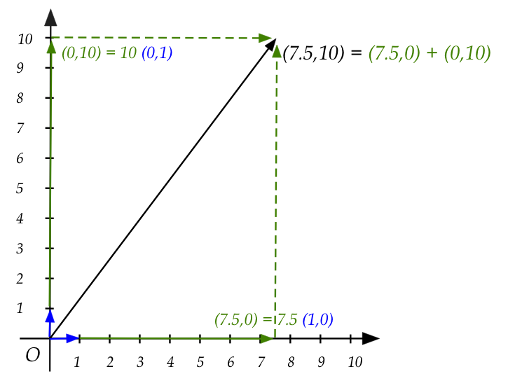
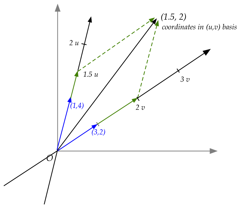
Coordinates
Let's review the meaning of coordinates in 2D:
To see how it can be useful, let's look at an example:
- Suppose we had the following data:
$$
\mat{1.1& 2.1& 2.8& 3.8& 5.1& 5.8& 7.2& 7.8\\
1.0& 1.9& 2.9& 4.1& 5.2& 6.1& 7.3& 8.1}
$$
- Think of the data as \((x_i,y_i)\) pairs, one per column.
- Let's now compute some stats
- The mean and variance of the first coordinate (of the \(x_i\)'s).
- The mean and variance of the second coordinate (of the \(y_i\)'s).
- The covariance.
In-Class Exercise 18:
Download ChangeOfBasisExample.java,
compile and execute to view the statistics before and after
a change-of-basis.
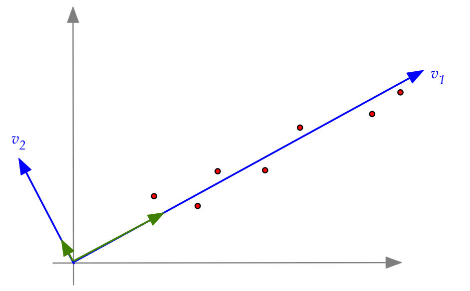
- Clearly, with the new basis, one can see that the
data is really "one dimensional."
\(\rhd\)
The new coordinates make that apparent
- The variance in the second coordinate is nearly zero.
- The new basis removes the correlation between the two coordinates.
- In this particular example, it's easy to see why by plotting
the data along with the new basis vectors.
In-Class Exercise 19:
Download DrawBasisExample.java,
compile and execute to view the points along with the new basis vectors.
Notice that the second coordinate is nearly zero.
- How do we choose a new basis and then compute coordinates in
that basis?
- We'll first (in this module) need to understand projections.
- Then, in a later module, we'll look at the PCA method for
creating a good basis.
7.7
Projection
Let's first examine a 2D example:
- Consider the vectors
$$\eqb{
{\bf w} & \eql & (4,3) \\
{\bf v} & \eql & (6,2)
}$$
and the shortest distance from the tip of \({\bf w}\) to the line
containing \({\bf v}\)
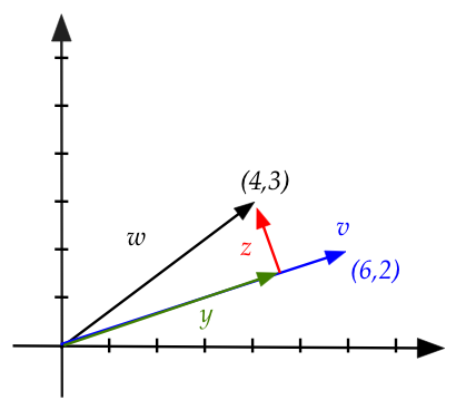
- This is the perpendicular from \({\bf w}\) to that line.
- There will be some scalar \(\alpha\) such that
\(\alpha{\bf v}\) ends at where the perpendicular meets the line.
- Define the vector
$$
{\bf z} \defn {\bf w} - \alpha{\bf v}
$$
- Since \({\bf z}\) is orthogonal to \({\bf v}\), the dot
product is zero:
$$
{\bf z} \cdot {\bf v} \eql 0\\
$$
Or
$$
({\bf w} - \alpha{\bf v}) \cdot {\bf v} \eql 0\\
$$
Which means
$$
\alpha \eql \frac{{\bf w} \cdot {\bf v}}{{\bf v} \cdot {\bf v}}
$$
- Note: \(\alpha\) is a scalar.
In-Class Exercise 20:
Calculate \(\alpha\) by hand for the example above.
Then, calculate \({\bf z}\) and verify that
\({\bf z} \cdot {\bf v} = 0\).
- Define the vector
$$\eqb{
{\bf y} & \eql & \mbox{projection of } {\bf w} \mbox{ on }
{\bf v}\\
& \eql & \alpha {\bf v}\\
& \eql & \left( \frac{{\bf w} \cdot {\bf v}}{{\bf v}
\cdot {\bf v}} \right) {\bf v}\\
}$$
- Sometimes we use the notation
$$
\mbox{proj}_{\bf v}({\bf w}) \eql \mbox{projection of } {\bf
w} \mbox{ on } {\bf v}
$$
In-Class Exercise 21:
For the same \({\bf w}\) as above but with \({\bf v}=(3,1)\)
use the code in
ProjectionExample.java
to compute \({\bf y}=\mbox{proj}_{\bf v}({\bf w})\).
What is the additional arrow (starting at the origin)?
A 3D example:
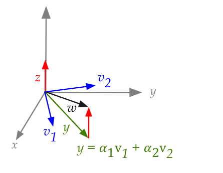
- Suppose that vectors \({\bf v}_1\) and \({\bf v}_2\) are
in the (x,y) plane and that they are orthogonal to each
other, i.e.,
$$
{\bf v}_1 \cdot {\bf v}_2 \eql 0
$$
- Note: \({\bf v}_1\) and \({\bf v}_2\) form a basis
for the plane.
- Next, let \({\bf w}\) be any 3D vector and let
$$
{\bf y} \eql \mbox{ projection of } {\bf w} \mbox{ on the (x,y)-plane}
$$
- This means the vector \({\bf y}\) is the closest in the
plane to \({\bf w}\).
- Since \({\bf y}\) is in the (x,y)-plane, it is a linear
combination of \({\bf v}_1\) and \({\bf v}_2\)
$$
{\bf y} \eql \alpha_1{\bf v}_1 + \alpha_2{\bf v}_2
$$
- Next,
$$\eqb{
{\bf z} & \eql & {\bf w} - {\bf y} \\
& \eql &
{\bf w} - \alpha_1{\bf v}_1 - \alpha_2{\bf v}_2
}$$
- Because \({\bf z}\) is orthogonal to the plane and therefore
to every vector in the plane,
$$\eqb{
{\bf z} \cdot {\bf v}_1 & \eql & 0\\
{\bf z} \cdot {\bf v}_2 & \eql & 0\\
}$$
- Substituting for \({\bf z}\)
$$\eqb{
({\bf w} - \alpha_1{\bf v}_1 - \alpha_2{\bf v}_2) \cdot
{\bf v}_1 & \eql & 0\\
({\bf w} - \alpha_1{\bf v}_1 - \alpha_2{\bf v}_2) \cdot
{\bf v}_2 & \eql & 0\\
}$$
- Which gives us
$$\eqb{
\alpha_1 & \eql & \frac{{\bf w} \cdot {\bf v}_1}{{\bf v}_1 \cdot {\bf v}_1}\\
\alpha_2 & \eql & \frac{{\bf w} \cdot {\bf v}_2}{{\bf v}_2 \cdot {\bf v}_2}\\
}$$
In-Class Exercise 22:
Fill in the key step in going from
\( ({\bf w} - \alpha_1{\bf v}_1 - \alpha_2{\bf v}_2) \cdot {\bf v}_1 = 0\)
to
\(\alpha_1 = \frac{{\bf w} \cdot {\bf v}_1}{{\bf v}_1 \cdot {\bf v}_1}\),
and show
why \({\bf v}_2\) disappears altogether
in the expression for \(\alpha_1\).
Download and execute Projection3D.java
to confirm that the code contains the above calculations. Change the
view to look down the z-axis and examine the stretched versions of
\({\bf v}_1\) and \({\bf v}_2\). What do these stretched versions add
up to?
- Thus, when \({\bf w}\) is NOT in the span of the \({\bf
v_i}\)'s, the scaled \({\bf v_i}\)'s add up to the projection
\({\bf y}\):
$$
{\bf y} \eql \alpha_1{\bf v}_1 + \alpha_2{\bf v}_2
$$
What happens when \({\bf w}\) IS in the span of the \({\bf v_i}\)'s?
- In the above 3D example, the vector \({\bf w}\) was outside
the span of \({\bf v}_1\) and \({\bf v}_2\) (which were in the x-y plane).
- In many cases, we have a vector \({\bf w}\) that's in the
span, whose coordinates we wish to compute with respect to
a different basis (like \({\bf v}_1\) and \({\bf v}_2\)).
- Consider
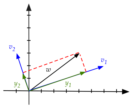
- Here, \({\bf w}\) is in the x-y plane along with
\({\bf v}_1\) and \({\bf v}_2\).
- Therefore we can write
$$
{\bf w} \eql \alpha_1{\bf v}_1 + \alpha_2{\bf v}_2
$$
- Since
$$
{\bf w}\cdot {\bf v}_1 \eql
(\alpha_1{\bf v}_1 + \alpha_2{\bf v}_2) \cdot {\bf v}_1 \eql
\alpha_1{\bf v}_1
$$
we can compute
$$
\alpha_1 \eql \frac{{\bf w} \cdot {\bf v}_1}{{\bf v}_1 \cdot {\bf v}_1}
$$
- Here, the projection vectors are
$$\eqb{
{\bf y}_1 & \eql & \mbox{proj}_{{\bf v}_1}({\bf w}) & \eql & \alpha_1 {\bf v}_1\\
{\bf y}_2 & \eql & \mbox{proj}_{{\bf v}_2}({\bf w}) & \eql & \alpha_2 {\bf v}_2\\
}$$
- Thus, the adding up of the stretched \({\bf v_i}\)'s
gives the original \({\bf w}\) and itself:
$$
{\bf w} \eql \alpha_1{\bf v}_1 + \alpha_2{\bf v}_2
$$
- Another way to remember this:
- Suppose \({\bf w}\)
is a vector in the span of an orthogonal basis (the \({\bf v_i}\)'s).
- Suppose we compute the projections \(\alpha_i {\bf v_i}\).
- Those projections are all we need to reconstruct \({\bf w}\)
by simple addition:
$$
{\bf w} \eql \sum_i \alpha_i {\bf v_i}
$$
This turns out to be useful in all kinds of applications
(example: Fourier transform).
Projection and coordinates:
- Now, the numbers \((\alpha_1,\alpha_2)\) above are the
coordinates of \({\bf w}\) with respect to the basis
\({\bf v}_1,{\bf v}_2\) because
$$
{\bf w} \eql \alpha_1{\bf v}_1 + \alpha_2{\bf v}_2
$$
- This can be generalized to any number of dimensions:
- Suppose \({\bf v}_1,{\bf v}_2,\ldots,{\bf v}_n\) is
an orthogonal basis for some space \({\bf W}\).
\(\rhd\)
Then, \({\bf v}_i \cdot {\bf v}_j = 0\).
- Let \({\bf w}\) be any vector in the space.
- Then, \({\bf w}\) can be expressed in terms of the \({\bf v}_i\)'s
$$
{\bf w} \eql \alpha_1 {\bf v}_1 + \alpha_2 {\bf v}_2
+ \ldots + \alpha_n {\bf v}_n
$$
where
$$
\alpha_i \eql \frac{{\bf w} \cdot {\bf v}_i}{{\bf v}_i \cdot {\bf v}_i}
$$
- If we did NOT have orthogonality, it would be more
complicated:
- Suppose the \({\bf v}_i\)'s are NOT orthogonal (but yet independent).
- Then suppose we want to express \({\bf w}\) in terms of the
\({\bf v}_i\)'s.
- Let
$$
{\bf w} \eql x_1 {\bf v}_1 + x_2 {\bf v}_2
+ \ldots + x_n {\bf v}_n
$$
- This is nothing but \({\bf Ax}={\bf b}\), or rather
\({\bf Ax}={\bf w}\).
- Which means the complicated
RREF algorithm, worrying about whether we get
a solution, and so on.
- But with an orthogonal collection of vectors, the
calculations are trivially easy. Each "stretch" is simply
$$
\alpha_i \eql \frac{{\bf w} \cdot {\bf v}_i}{{\bf v}_i \cdot {\bf v}_i}
$$
- The stretched vector along each \({\bf v}_i\) direction,
\(\alpha_i {\bf v}_i\) is the projection of \({\bf w}\)
in that direction:
$$\eqb{
\mbox{proj}_{{\bf v}_i}({\bf w})
& \eql & \alpha_i {\bf v}_i\\
& \eql & \left( \frac{{\bf w} \cdot {\bf v}_i}{{\bf v}_i
\cdot {\bf v}_i} \right) {\bf v}_i\\
}$$
- Two cases:
- If \({\bf w}\) is in the span of the \({\bf v}_i\)'s then
the sum of its projections along the \({\bf v}_i\)'s
is \({\bf w}\) itself:
$$
\mbox{proj}_{{\bf v}_1}({\bf w}) +
\mbox{proj}_{{\bf v}_2}({\bf w}) +
\ldots +
\mbox{proj}_{{\bf v}_n}({\bf w})
\eql
{\bf w}
$$
- Otherwise, if \({\bf w}\) is NOT in the
span of the \({\bf v}_i\)'s then the sum projections
gives us the closest vector in the span:
$$
\mbox{proj}_{{\bf v}_1}({\bf w}) +
\mbox{proj}_{{\bf v}_2}({\bf w}) +
\ldots +
\mbox{proj}_{{\bf v}_n}({\bf w})
\eql
{\bf y}
$$
where \({\bf y}\) is the projection of \({\bf w}\)
on the space spanned by \({\bf v}_1,\ldots,{\bf v}_n\).
In-Class Exercise 23:
Suppose \({\bf w}=(4,3)\),
\({\bf v}_1=(6,2)\) and \({\bf v}_2=(-1,3)\).
Do the following by hand:
- Show \({\bf v}_1\) and \({\bf v}_2\) form an orthogonal basis.
- Find the coordinates of \({\bf w}\) in the basis.
- Find the projection vectors.
- Add the projection vectors to get \({\bf w}\).
Confirm your calculations by adding code to
ProjectionExample2.java.
Let's summarize what we've learned (for the case
\({\bf w} \in \mbox{span}( {\bf v}_1,\ldots, {\bf v}_1)\)):
:
We will later address the question of finding a "good" orthogonal basis.
For now, we'll look at a more basic problem: given any collection
of vectors that span a space, how do we even find any
orthogonal basis?
\(\rhd\)
This is the famous Gram-Schmidt algorithm (next).
The algorithm will help us with something even more important:
the QR decomposition.
7.8
The Gram-Schmidt algorithm
The G-S algorithm tries to solve the following problem:
First, some intuition with \(n=2\)
- In this case we have two vectors \({\bf w}_1, {\bf w}_2\)
and the dimension is 2
\(\rhd\)
Our familiar 2D space.
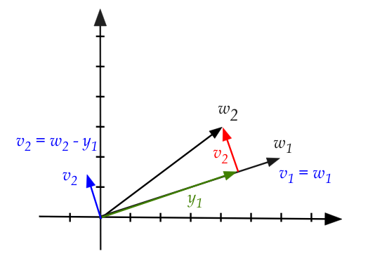
- First, observe that \({\bf w}_1, {\bf w}_2\) are not orthogonal.
- We need to find \({\bf v}_1, {\bf v}_2\) that are.
- We'll pick \({\bf v}_1\) to be \({\bf w}_1\).
- Therefore we need to find some \({\bf v}_2\) that's
orthogonal to \({\bf v}_1 = {\bf w}_1\).
- Observe that \(\mbox{proj}_{{\bf v}_1}({\bf w}_2)\)
goes along \({\bf v}_1\).
\(\rhd\)
That's what a projection is.
- Therefore
$$
{\bf w}_2 - \mbox{proj}_{{\bf v}_1}({\bf w}_2)
$$
is orthogonal to \({\bf v}_1\).
- We will define this to be \({\bf v}_2\):
$$
{\bf v}_2 \defn {\bf w}_2 - \mbox{proj}_{{\bf v}_1}({\bf w}_2)
$$
- We now have two orthogonal vectors that span the space.
In-Class Exercise 26:
Download, compile and execute
GramSchmidt.java
to first draw the vectors
\({\bf w}_1=(6,2), {\bf w}_2=(4,3)\).
Then, examine the section that performs the
projection-subtraction to compute \({\bf v}_2\).
To generalize, let's make this idea work for 3D:
- We are given three vectors \({\bf w}_1, {\bf w}_2,{\bf w}_3\)
that aren't necessarily orthogonal.
- We need find \({\bf v}_1, {\bf v}_2,{\bf v}_3\) so that
these are an orthogonal basis for the same space.
- Start by defining \({\bf v}_1 = {\bf w}_1\).
- As before, we'll compute \({\bf v}_2\) by subtracting
off the projection of \({\bf w}_2\) on \({\bf v}_1\)
$$
{\bf v}_2 \defn {\bf w}_2 - \mbox{proj}_{{\bf v}_1}({\bf w}_2)
$$
- The next vector, \({\bf v}_3\), needs to be orthogonal to
both \({\bf v}_1\) and \({\bf v}_2\).
- Therefore it will be orthogonal to any linear combination
of \({\bf v}_1\) and \({\bf v}_2\).
\(\rhd\)
That is, orthogonal to any vector in \(\mbox{span}({\bf v}_1,{\bf v}_2)\).
- We need a name for this subspace. We'll call it
$$
{\bf V}_2 \eql \mbox{span}({\bf v}_1,{\bf v}_2)
$$
- How do we find a vector \({\bf v}_3\) orthogonal to \({\bf V}_2\)?
- Consider \({\bf w}_3\)'s projection onto the plane
\({\bf V}_2\):
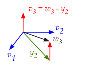
- Call the projection \({\bf y}_2\).
- Since \({\bf y}_2\) is directly below, the
subtraction \({\bf w}_3 - {\bf y}_2\) is orthogonal to the plane.
- This is our \({\bf v}_3\)!
- How did we compute \({\bf y}_2\) earlier?
$$\eqb{
{\bf y}_2 & \eql & \mbox{ sum of projections of } {\bf w}_3
\mbox{ on } {\bf v}_1
\mbox{ and } {\bf v}_2\\
& \eql &
\mbox{proj}_{{\bf v}_1}({\bf w}_3)
+
\mbox{proj}_{{\bf v}_2}({\bf w}_3)\\
& \eql &
\left( \frac{{\bf w}_3 \cdot {\bf v}_1}{{\bf v}_1
\cdot {\bf v}_1} \right) {\bf v}_1
+
\left( \frac{{\bf w}_3 \cdot {\bf v}_2}{{\bf v}_2
\cdot {\bf v}_2} \right) {\bf v}_2
}$$
Recall: this is from the case where \({\bf w}_3\) is not
in the span of \({\bf v}_1, {\bf v}_2\).
- Thus,
$$\eqb{
{\bf v}_3 & \eql & {\bf w}_3 - {\bf y}_2 \\
& \eql &
{\bf w}_3 -
\left( \frac{{\bf w}_3 \cdot {\bf v}_1}{{\bf v}_1
\cdot {\bf v}_1} \right) {\bf v}_1
-
\left( \frac{{\bf w}_3 \cdot {\bf v}_2}{{\bf v}_2
\cdot {\bf v}_2} \right) {\bf v}_2
}$$
- A useful interpretation:
- Each amount being subtracted above is a projection.
- The first is a projection on \({\bf v}_1\).
- The second is a projection on \({\bf v}_2\).
- Thus, each successive \({\bf v}_i\) is obtained by
subtracting off the projections on all previous \({\bf v}_j\)'s.
- Why does this work?
- The real projection that needs to be subtracted is the
projection on to the subspace of all previous \({\bf v}_j\)'s.
- This projection is the sum of projections on each
individual \({\bf v}_j\).
\(\rhd\)
This is the convenience we get from terms that "disappear"
because of orthogonality.
In-Class Exercise 27:
Download, compile and execute
GramSchmidt3D.java
to first draw three vectors
\({\bf w}_1=(6,2,4), {\bf w}_2=(4,3,1),{\bf w}_3=(1,2,6)\).
Then, un-comment the section that performs the
sequence of projection-subtractions to compute
orthogonal vectors \({\bf v}_2,{\bf v}_3\).
We now have an algorithm (Gram-Schmidt) for the general case:
- The input is a linearly independent collection
\({\bf w}_1, {\bf w}_2, \ldots, {\bf w}_n\).
- We need an orthogonal basis
\({\bf v}_1, {\bf v}_2, \ldots, {\bf v}_n\).
- We'll use the notation \({\bf V}_k\) to denote the subspace
$$
{\bf V}_k \eql \mbox{span}({\bf v}_1, {\bf v}_2, \ldots, {\bf v}_k)
$$
- Start with
$$
{\bf v}_1 \defn {\bf w}_1
$$
- Then,
$$\eqb{
{\bf v}_k & \defn & {\bf w}_k -
\mbox{proj}_{{\bf V}_{k-1}}({\bf w}_k)\\
& \eql &
{\bf w}_k -
\left( \frac{{\bf w}_k \cdot {\bf v}_1}{{\bf v}_1
\cdot {\bf v}_1} \right) {\bf v}_1
-
\left( \frac{{\bf w}_k \cdot {\bf v}_1}{{\bf v}_2
\cdot {\bf v}_2} \right) {\bf v}_2
- \ldots -
\left( \frac{{\bf w}_k \cdot {\bf v}_{k-1}}{{\bf v}_{k-1}
\cdot {\bf v}_{k-1}} \right) {\bf v}_{k-1}
}$$
- Let's define the notation
$$
c_{jk} \defn \left( \frac{{\bf w}_k \cdot {\bf v}_j}{{\bf v}_j
\cdot {\bf v}_j} \right)
$$
- Then
$$\eqb{
{\bf v}_k
& \eql &
{\bf w}_k -
\left( \frac{{\bf w}_k \cdot {\bf v}_1}{{\bf v}_1
\cdot {\bf v}_1} \right) {\bf v}_1
-
\left( \frac{{\bf w}_k \cdot {\bf v}_2}{{\bf v}_2
\cdot {\bf v}_2} \right) {\bf v}_2
- \ldots -
\left( \frac{{\bf w}_k \cdot {\bf v}_{k-1}}{{\bf v}_{k-1}
\cdot {\bf v}_{k-1}} \right) {\bf v}_{k-1}\\
& \eql &
{\bf w}_k -
c_{1k} {\bf v}_1
-
c_{2k} {\bf v}_2
- \ldots -
c_{k-1,k} {\bf v}_{k-1}\\
& \eql &
{\bf w}_k - \sum_{j=1}^{k-1} c_{jk} {\bf v}_j
}$$
- In pseudocode:
     Algorithm: gramSchmidt (A)
     Input: n vectors w1,..., wn as columns of matrix A
     1.   v1 = w1
     2.   for k=2 to n
     3.       s = 0
     4.       for j=1 to k-1
     5.           cjk = (wk  · vj) / vj · vj)
     6.           sj = cjk vj
     7.           s = s + sj
     8.       endfor
     9.       vk = wk - s
     10.  endfor

     11.  return v1,..., vn
When do we use Gram-Schmidt?
- Numerical computations tend to be more stable if orthogonal
bases are used.
- There are modifications that improve the G-S algorithm,
in the province of a course on numerical linear algebra.
- For our purposes in this course, the G-S algorithm leads
to the QR decomposition.
- Which is the foundation for algorithms that find eigenvectors.
7.9
The QR decomposition
In this and the remaining sections we will touch upon some advanced
topics, included here for completeness and awareness.
Orthogonal vs orthonormal:
A small twist:
The QR Decomposition:
About the matrix \({\bf Q}\):
- The term orthogonal matrix is used when the columns
are orthonormal.
- Since the columns of \({\bf Q}\) are the normalized
\({\bf u}_i\)'s, \({\bf Q}\) is an orthogonal matrix.
- Recall that for any orthogonal matrix \({\bf Q}\):
$$
{\bf Q}^T {\bf Q} \eql {\bf I}
$$
and therefore
$$
{\bf Q}^{-1} \eql {\bf Q}^T
$$
(another reason orthogonal matrices are convenient).
- So, multiplying both sides of \({\bf A} = {\bf QR}\) by
\({\bf Q}^T\)
$$
{\bf R} \eql {\bf Q}^T {\bf A}
$$
which is another way of computing \({\bf R}\), after Gram-Schmidt.
An important property about \({\bf R}\):
Let's summarize the QR factorization with a theorem statement:
- Theorem 7.3:
Any matrix \({\bf A}\) with linearly independent columns can be factored into
a product \({\bf A}={\bf QR}\) where:
- \({\bf Q}\) is orthogonal.
- The columns of \({\bf Q}\) are an orthonormal basis for
the column space of \({\bf A}\).
- The matrix \({\bf R}\) is upper-triangular, invertible, and
has positive diagonal entries.
Lastly, we point out that it is possible to QR-factorize a matrix
whose columns aren't all necessarily independent:
- Suppose \({\bf A}\) is any matrix with \(m \geq n\).
- Identify the independent columns using the 2nd (column) method
with the RREF.
- Replace the dependent columns with new columns so that all
columns are independent. Call this matrix \({\bf A}^\prime\)
- Find the \({\bf Q}\) for \({\bf A}^\prime\) using Gram-Schmidt.
- Define \({\bf R}={\bf Q}^T {\bf A}\) so that
\({\bf A}={\bf QR}\).
- It can be shown that the \({\bf R}\) so obtained is
partly upper-triangular.
7.10
Least squares revisited
Recall the least squares equation:
$$
\hat{\bf x}
\eql
({\bf A}^T {\bf A})^{-1}
{\bf A}^T {\bf b}
$$
The computation involves transposes, matrix multiplications,
and computing the inverse of \({\bf A}^T {\bf A}\).
Using QR for least squares:
7.11
Properties of orthogonal matrices
We close this module with a few observations about orthogonal
matrices.
First, let's revisit the unfortunate nomenclature and clarify:
- An orthogonal matrix has orthonormal columns.
- Why isn't this called an orthonormal matrix?
It probably should, but the terminology has stuck.
- We'll break with tradition and use orthonormal matrix just to clarify.
- What do you call a matrix whose columns are orthogonal
but not necessarily orthonormal (i.e., non-unit-length)?
Since there's no special name, we'll just say "orthogonal columns".
Perhaps the most useful is one we've seen before: if \({\bf Q}\)
is an orthonormal matrix, \({\bf Q}^{-1} = {\bf Q}^T\).
Length and dot-product preservation:
- Recall from Module 4:
- Reflection and rotation are orthonormal
- We generated random orthonormal matrices and applied them to vectors.
- The transformed vector's length was unchanged.
Theorem 7.4: The following are equivalent:
- \({\bf Q}\) has orthonormal columns.
- \(|{\bf Qx}| \eql |{\bf x}|\)
\(\rhd\)
Transformation by \({\bf Q}\) preserves lengths.
- \(({\bf Qx}) \cdot ({\bf Qy}) \eql
{\bf x}\cdot{\bf y}\)
\(\rhd\)
Transformation by \({\bf Q}\) preserves dot-products
- Before the proof, we'll first need to clarify something
about transposes and vectors:
- Proof of Theorem 7.4: We'll show this in three parts: \(1 \Rightarrow 2 \Rightarrow 3
\Rightarrow 1\).
- \((1\;\Rightarrow\; 2)\) Here, we start with the assumption
that \({\bf Q}\) has orthonormal columns and want to show that
transformation by \({\bf Q}\) preserves length.
Observe that \(|{\bf u}|^2 = {\bf u}^T {\bf u}\) for any vector
\({\bf u}\). Thus
$$\eqb{
|{\bf Qx}|^2 & \eql & ({\bf Qx})^T ({\bf Qx}) \\
& \eql &
{\bf x}^T {\bf Q}^T {\bf Q} {\bf x} \\
& \eql &
{\bf x}^T {\bf I} {\bf x} \\
& \eql &
{\bf x}^T {\bf x} \\
& \eql &
|{\bf x}|^2
}$$
- \((2\;\Rightarrow\; 3)\) For this, we start with the
assumption that \({\bf Q}\) preserves lengths and wish to
show that it preserves dot products. This turns out to be
surprisingly tricky. We will show this in two steps
- Step 1: \(|{\bf Q}({\bf x}+{\bf y})|^2 = |{\bf x}+{\bf
y}|^2 \).
- Step 2: Use Step 1 and Part(1) above to prove
\(({\bf Qx}) \cdot ({\bf Qy}) \eql
{\bf Q}({\bf x}\cdot{\bf y})\)
Let's start with Step 1. Note that
$$\eqb{
|{\bf x}+{\bf y}|^2
& \eql &
({\bf x}+{\bf y})^T ({\bf x}+{\bf y}) \\
& \eql &
({\bf x}^T +{\bf y}^T) ({\bf x}+{\bf y}) \\
& \eql &
|{\bf x}|^2 + 2 {\bf x}^T {\bf y}
+ |{\bf y}|^2\\
}$$
We can similarly expand
$$\eqb{
|{\bf Q}({\bf x}+{\bf y})|^2
& \eql &
|{\bf Qx}|^2 + 2 ({\bf Qx})^T ({\bf Qy})
+ |{\bf Qy}|^2\\
& \eql &
|{\bf x}|^2 + 2 ({\bf Qx})^T ({\bf Qy})
+ |{\bf y}|^2 \\
& \eql &
|{\bf x}|^2 + 2 {\bf x}^T {\bf Q}^T {\bf Qy}
+ |{\bf y}|^2 \\
& \eql &
|{\bf x}|^2 + 2 {\bf x}^T {\bf y}
+ |{\bf y}|^2 \\
}$$
which is the same as the last line in the expansion
of \(|{\bf x}+{\bf y}|^2\).
Now for Step 2. First, observe that for any two
vectors \({\bf u}\) and \({\bf v}\)
$$\eqb{
({\bf u} + {\bf v})^2
& \eql &
({\bf u} + {\bf v}) \cdot ({\bf u} + {\bf v})
& \eql &
{\bf u}\cdot{\bf u} + 2{\bf u}\cdot{\bf v}
+ {\bf v}\cdot{\bf v} \\
({\bf u} - {\bf v})^2
& \eql &
({\bf u} - {\bf v}) \cdot ({\bf u} - {\bf v})
& \eql &
{\bf u}\cdot{\bf u} - 2{\bf u}\cdot{\bf v}
+ {\bf v}\cdot{\bf v}
}$$
Therefore,
$$\eqb{
{\bf u}\cdot{\bf v}
& \eql &
\frac{1}{4} \left( ({\bf u} + {\bf v})^2 - ({\bf u} - {\bf v})^2 \right)\\
& \eql &
\frac{1}{4} \left( |{\bf u} + {\bf v}|^2 - |{\bf u} - {\bf
v}|^2 \right) \\
}$$
And so, with \({\bf u}={\bf Qx}\) and \({\bf v}={\bf Qy}\)
$$\eqb{
({\bf Q}{\bf x})\cdot ({\bf Q}{\bf y})
& \eql &
\frac{1}{4} (|{\bf Q}{\bf x} + {\bf Q}{\bf y}|^2 - |{\bf Q}{\bf x} - {\bf Q}{\bf y}|^2)\\
& \eql &
\frac{1}{4} (|{\bf Q}({\bf x} + {\bf y})|^2 - |{\bf Q}({\bf x} - {\bf y})|^2)\\
& \eql &
\frac{1}{4} (|{\bf x} + {\bf y}|^2 - |{\bf x} - {\bf y}|^2)\\
}$$
using Step 1. The last expression above is equal to
\({\bf x}\cdot{\bf y}\)
and so
\(({\bf Qx}) \cdot ({\bf Qy}) \eql
{\bf Q}({\bf x}\cdot{\bf y})\)
- \((3\;\Rightarrow\; 1)\) For this part, we want to show
that if \({\bf Q}\) preserves dot-products, it must be
orthonormal.
Let \({\bf e}_i=(0,\ldots,0, 1, 0,\ldots,0) \) be the i-th
standard basis vector (with a 1 in the i-th place).
Notice that \({\bf Q} {\bf e}_i\) is the i-th column of \({\bf Q}\).
Thus,
$$
({\bf Q} {\bf e}_i) \cdot ({\bf Q} {\bf e}_j)
\eql \left\{
\begin{array}{ll}
1 & \;\;\;\;\;\; \mbox{if } i=j\\
0 & \;\;\;\;\;\; \mbox{if } i\neq j\\
\end{array}
\right.
$$
In-Class Exercise 33:
Fill in the few steps left out:
- Show that \({\bf Q} {\bf e}_i\) is the i-th column of \({\bf Q}\).
- Show why \(({\bf Q} {\bf e}_i) \cdot ({\bf Q} {\bf e}_j)\)
is either 1 or 0, depending on whether \(i=j\).
- Corollary 7.5:
Multiplication of two vectors separately by an orthonormal matrix
preserves the angle between them.
In-Class Exercise 34:
Use Theorem 7.4 to prove Corollary 7.5. Hint:
express the angle in terms of the dot product and lengths.
- An orthonormal matrix is sometimes called a generalized
rotation or reflection matrix because it preserves lengths and angles.
- A theoretical result that aligns with this notion is the
following, which we will state without proof.
- Proposition 7.6:
An \(n\times n\) orthonormal matrix can be written as the product
of \(k\) reflection matrices where \(k\leq n\).
- Another nice property concerns the product of orthonormal matrices.
- Proposition 7.7:
The product of two orthonormal matrices is orthonormal.
Proof: If \({\bf A}\) and \({\bf B}\) are
orthonormal then
\(({\bf A} {\bf B})^T ({\bf A} {\bf B}) =
{\bf B}^T {\bf A}^T {\bf A} {\bf B} =
{\bf B}^T {\bf B} = {\bf I}\)
which makes \({\bf A} {\bf B}\) orthonormal.
- The earlier result about projections can be elegantly stated
in matrix form.
- Proposition 7.8:
Let \({\bf b}\) be a vector in \(\mathbb{R}^n\) and
\({\bf W}\) be a subspace with an orthonormal basis
\({\bf u}_1, {\bf u}_2, \ldots, {\bf u}_k\) forming
the columns of \({\bf Q}\). Then the projection of the
vector \({\bf b}\) on the subspace \({\bf W}\) is
$$
{\bf y} \eql \mbox{proj}_{{\bf W}} ({\bf b}) \eql {\bf QQ}^T {\bf b}
$$
Proof:
Since \({\bf y}\) is in the subspace, it can be expressed as a
linear combination of the basis vectors:
$$\eqb{
{\bf y}
& \eql &
x_1 {\bf u}_1 + x_2 {\bf u}_2 + \ldots + x_k {\bf u}_k\\
& \eql &
{\bf Qx}
}$$
where \({\bf x}=(x_1,\ldots,x_n)\). In developing the Gram-Schmidt
algorithm, we showed that
$$\eqb{
{\bf y}
& \eql &
\frac{{\bf b} \cdot {\bf u}_1}{{\bf u}_1\cdot {\bf u}_1}
{\bf u}_1
+
\frac{{\bf b} \cdot {\bf u}_2}{{\bf u}_2\cdot {\bf u}_2}
{\bf u}_2
+ \ldots +
\frac{{\bf b} \cdot {\bf u}_k}{{\bf u}_k\cdot {\bf u}_k}
{\bf u}_k \\
& \eql &
({\bf b} \cdot {\bf u}_1) {\bf u}_1
+
({\bf b} \cdot {\bf u}_2) {\bf u}_2
+ \ldots +
({\bf b} \cdot {\bf u}_k) {\bf u}_k \\
& \eql &
({\bf u}^T_1 \cdot {\bf b} ) {\bf u}_1
+
({\bf u}^T_2 \cdot {\bf b} ) {\bf u}_2
+ \ldots +
({\bf u}^T_k \cdot {\bf b} ) {\bf u}_k
}$$
Which means
$$
{\bf x} \eql
\mat{x_1 \\ x_2 \\ \vdots \\ x_k}
\eql
\mat{
{\bf u}^T_1 \cdot {\bf b} \\
{\bf u}^T_2 \cdot {\bf b} \\
\vdots\\
{\bf u}^T_k \cdot {\bf b}
}
\eql
{\bf Q}^T {\bf b}
$$
Substituting for \({\bf x}\) in \({\bf y}={\bf Qx}\) completes
the proof. \(\;\;\;\;\Box\).
7.12
Highlights and study tips
This module was a little more abstract and went deeper into
linear algebra.
Some highlights:
- There were several aspects of orthogonality:
- Two vectors can be orthogonal to each other.
- A vector can be orthogonal to an entire subspace
\(\rhd\)
That is, to all the vectors in the subspace.
- A collection of vectors can be mutually orthogonal.
- A matrix can be orthogonal (if it's columns are).
- An approximate solution to \({\bf Ax}={\bf b}\) was
cast as follows:
- Since there's no solution, \({\bf b}\) is not
in the column space of \({\bf A}\)
- We sought the linear combination of columns \({\bf A}\hat{x}\)
that's closest to \({\bf b}\).
- This is the projection of \({\bf b}\) onto the subspace
defined by the columns.
- This is the popular and extremely use least-squares
approach whose discoverer, Gauss, showed how powerful it was.
- In a curve or line-fitting problem, there are usually
too many points.
- Which means too many equations (and no exact solution).
- The "best" approximate solution is the one closest to the "target"
- By using the actual data to set up the "target" we reframe
curve-fitting as an equation-solution problem.
- We then saw that a projection onto a subspace is easily
computed if we have an orthogonal basis.
\(\rhd\)
Using simple dot-products (because the other terms vanish).
- This led to the Gram-Schmidt algorithm for finding an
orthonormal basis.
- Along the way, we compute the scalars to express the
the non-orthonormal basis
\(\rhd\)
This turned out to be the QR factorization.
- The QR factorization resulted in another way to solve
least squares that's more efficient. And has better numerical
properties, it turns out.
- Finally, orthonormal matrices have some nice properties that
will turn out to be useful in various occasions.
Study tips:
- This was a challenging module with some hairy expressions.
- Start with reviewing the arguments leading to the
least-squares method.
- The actual final expression is less important.
- To understand how to apply it, work through the
application to fitting a plane. See if you can eventually do this
without referring to the notes.
- Skip the details of the ellipse if that's too complicated.
- The notion of coordinates with respect to a basis is
important. Worth re-reading a few times.
- Work through the 2D and 3D projection examples carefully.
- The ideas leading up to Gram-Schmidt are more important than
the algorithm itself.
- The details of the QR factorization are challenging, but
it's a good idea to remember that such a factorization exists.
- The properties of orthonormal matrices are worth remembering
because they show up in other places.