Module objectives
By the end of this module, you should be able to
- Explain the terms linear independence (LI), rank, basis.
- Describe the connection between LI as defined for vectors
and matrix rank.
- Explain the significance of pivot rows and columns in the RREF.
- Construct a basis given a set of vectors.
- Prove many of the key results by yourself.
6.0
A matrix as data
Multivariate data:
- In many applications, one measures a number of variables
simultaneously.
- For example: a weather measurement at a location could
include these 6 variables: temperature, pressure, wind, humidity, cloud cover, precipitation.
- Assuming all the measurements can be converted to numeric
form, each measurement of a set of variables can be treated as a vector.
- For example, suppose the following six measurements
of some 6-variable system
were made at a certain time: \(12.5, 13.5, 15.25, 12.55, 13, 11.5\).
- This is a single, multivariate data sample.
- Then, we might get another sample of the six quantities, such as
\(13.2, 13.5, 16.65, 12.69, 14.4, 11.85\).
- We will place each sample as a column in a matrix.
- Thus, the above two samples would look like:
$$
\mat{
12.5 & 13.2 \\
13.5 & 13.5 \\
15.25 & 16.65 \\
12.55 & 12.69 \\
13 & 14.4 \\
11.5 & 11.85 \\
}
$$
- Here is an example with 8 samples, each as one column
in the data matrix we're calling \({\bf X}\):
$$
{\bf X} \eql
\mat{
12.500 & 13.200 & 12.270 & 13.710 & 14.781 & 12.299 & 10.134 & 8.962\\
13.500 & 13.500 & 12.600 & 14.400 & 16.080 & 12.384 & 9.197 & 7.488\\
15.250 & 16.650 & 13.440 & 19.020 & 23.682 & 13.174 & 4.063 & -0.845\\
12.550 & 12.690 & 12.234 & 13.062 & 13.780 & 12.175 & 10.786 & 10.039\\
13.000 & 14.400 & 12.540 & 15.420 & 17.562 & 12.598 & 8.268 & 5.923\\
11.500 & 11.850 & 11.835 & 11.655 & 11.351 & 11.957 & 12.468 & 12.737
}
$$
- We'll use this notation:
- Let \({\bf x}_i = \) the i-th column.
- \({\bf x}_i(j) = \) the j-th entry in the i-th column.
- For example:
$$
{\bf x}_3 \eql
\mat{12.270\\ 12.600\\ 13.440\\ 12.234\\ 12.540\\ 11.835}
$$
and
\({\bf x}_3(5) \eql 12.540\).
- Thus, the data matrix \({\bf X}\) consisting of
\(n\) samples, each of dimenion \(m\) can be viewed as
$$
{\bf X} \eql
\mat{
& & & \\
\vdots & \vdots & \ldots & \vdots \\
{\bf x}_1 & {\bf x}_2 & \ldots & {\bf x}_n\\
\vdots & \vdots & \ldots & \vdots \\
& & &
}
$$
where each column vector has \(m\) elements (numbers)
$$
{\bf x}_i = ({\bf x}_i(1), {\bf x}_i(2), \ldots, {\bf x}_i(m))
$$
Why place data into a matrix?
- We will later, when studying the singular value decomposition (SVD),
see that linear algebra techniques are the key to applications
like latent semantic analysis, recommendation engines, and image search.
- As an example, let's apply the RREF algorithm to the above
\(6 \times 8\) matrix to get:
$$
RREF({\bf X}) \eql
\mat{
1 & 0 & 0 & 0.60 & 1.55 & -0.36 & -1.97 & -2.82\\
0 & 1 & 0 & 1.40 & 2.32 & 0.12 & -1.81 & -2.86 \\
0 & 0 & 1 & -1 & -2.87 & 1.24 & 4.78 & 6.68 \\
0 & 0 & 0 & 0 & 0 & 0 & 0 & 0 \\
0 & 0 & 0 & 0 & 0 & 0 & 0 & 0 \\
0 & 0 & 0 & 0 & 0 & 0 & 0 & 0 }
$$
We see that some rows have "disappeared".
That is, the data appears reduced to three rows.
- The matrix is what we'd call a low rank matrix,
as opposed to a full rank matrix.
- Later, we will apply the SVD to the matrix to get
transformed data \({\bf Y}\):
$$
{\bf Y} \eql
\mat{
32.08 & 33.77 & 30.59 & 35.94 & 40.26 & 30.44 & 21.91 & 17.31\\
0.49 & 1.36 & -0.95 & 3.15 & 6.64 & -1.2 & -7.98 & -11.63\\
-0.66 & 0.31 & -0.14 & 0.17 & 0.09 & 0.1 & 0.08 & 0.05\\
0 & 0 & 0 & 0 & 0 & 0 & 0 & 0 \\
0 & 0 & 0 & 0 & 0 & 0 & 0 & 0 \\
0 & 0 & 0 & 0 & 0 & 0 & 0 & 0 }
$$
We see that the magnitudes of the numbers in the first row
dwarf the others, suggesting some type of importance.
This will turn out to be an effective way
to reduce the dimension of data sets.
- But as background to understanding the SVD, we'll first
need to understand the concepts of linear independence,
rank and basis.
6.1
Linearly independent vectors
Consider this example:
- Suppose we have three vectors
$$
{\bf u} \eql \vecthree{2}{-1}{1}
\;\;\;\;\;\;\;\;\;\;\;\;\;\;\;\;\;\;
{\bf v} \eql \vecthree{0}{1}{1}
\;\;\;\;\;\;\;\;\;\;\;\;\;\;\;\;\;\;
{\bf w} \eql \vecthree{6}{1}{7}
$$
and ask the question are there scalars \(\alpha, \beta\) such
that
$$
{\bf w} \eql \alpha {\bf u} + \beta {\bf v}?
$$
That is, can \({\bf w}\) be expressed as a linear combination of
\({\bf u}\) and \({\bf v}\)?
In-Class Exercise 1:
How does one address the question for the above example?
- With the above exercise, you saw that,
\({\bf w}\) can indeed be expressed as a linear combination of
\({\bf u}\) and \({\bf v}\):
$$
{\bf w} \eql 3 {\bf u} + 4 {\bf v}?
$$
Here, \(\alpha = 3, \beta=4\).
In-Class Exercise 2:
Can \({\bf u}\) be expressed in terms of \({\bf v}\)
and \({\bf w}\)?
- On the other hand \({\bf z}=(6,1,8)\) cannot be
expressed as a linear combination of
\({\bf u}\) and \({\bf v}\).
In-Class Exercise 3:
Show that this is the case.
In-Class Exercise 4:
Can \({\bf u}\) above be expressed as a linear combination
of \({\bf v}\) and \({\bf z}\)? Or
\({\bf v}\) as a linear combination
of \({\bf u}\) and \({\bf z}\)?
- One could say \({\bf w}\) depends in a linear
fashion on \({\bf u}\) and \({\bf v}\).
- Similarly, there is no way that
\({\bf z}\) is linearly dependent on \({\bf u}\) and \({\bf v}\).
We are led to a definition of linear independence:
- One way to define linear independence is to first
define dependence for a particular vector, along the lines of:
\({\bf w}\) is linearly dependent on
\({\bf v}_1, {\bf v}_2, \ldots, {\bf v}_n\)
if there exist scalars \(\alpha_1,\alpha_2,\ldots,\alpha_n\)
such that
$$
{\bf w} \eql \alpha_1 {\bf v}_1 + \alpha_2 {\bf v}_2
+ \ldots + \alpha_n {\bf v}_n
$$
- Observe:
we can algebraically rearrange to see that
$$
{\bf v}_2 \eql \beta_1 {\bf v}_1 + \beta_2 {\bf w}
+ \ldots + \beta_n {\bf v}_n
$$
(for a different set of coefficients)
- That is, there's nothing one-directional about
\({\bf w}\)'s dependence.
- Once one variable is dependent on others, they all are.
- Therefore, it's often more useful to define linear
independence directly, and for a collection of vectors.
- Definition:
Vectors \({\bf v}_1, {\bf v}_2, \ldots, {\bf v}_n\)
are linearly independent if the only
solution to the equation
$$
\alpha_1 {\bf v}_1 + \alpha_2 {\bf v}_2 + \ldots + \alpha_n {\bf v}_n
\eql {\bf 0}
$$
is \(\alpha_1 = \alpha_2 = \ldots = \alpha_n = 0\).
- Let's see how this works for an individual vector in
the collection:
- Suppose \({\bf v}_1\) were linearly dependent on the others.
- Then, we'd be able to write
$$
{\bf v}_1 = \beta_2 {\bf v}_2 + \ldots + \beta_n {\bf v}_n
$$
- Then,
$$
- {\bf v}_1 + \beta_2 {\bf v}_2 + \ldots + \beta_n {\bf v}_n
\eql {\bf 0}
$$
implies that at least one coefficient (that of \({\bf v}_1\))
is not zero.
- This is consistent with the definition.
- Another way of thinking about it:
- Suppose we have
$$
\alpha_1 {\bf v}_1 + \alpha_2 {\bf v}_2 + \ldots + \alpha_n {\bf v}_n
\eql {\bf 0}
$$
where at least one \(\alpha_i \neq 0\).
- Suppose, for example, \(\alpha_2 \neq 0\) (among possibly
other non-zero scalars).
- Then, we could write
$$
- \alpha_2 {\bf v}_2 \eql \alpha_1 {\bf v}_1 + \ldots + \alpha_n {\bf v}_n
$$
- Which, because \(\alpha_2 \neq 0\), means that we can divide:
$$
{\bf v}_2 \eql \frac{\alpha_1}{-\alpha_2} {\bf v}_1 + \ldots + \frac{\alpha_n}{-\alpha_2} {\bf v}_n
$$
- That is, \({\bf v}_2\) is dependent on the other vectors.
- The weirdness of the zero vector:
- Suppose \({\bf v}_1 = {\bf 0} = (0,0,...,0)\).
- Then, consider
$$
{\bf v}_1 = \beta_2 {\bf v}_2 + \ldots + \beta_n {\bf v}_n
$$
- Here, we can make \(\beta_2 = \beta_3 = ... = \beta_n = 0\) so that
$$
{\bf 0} = 0 {\bf v}_2 + \ldots + 0 {\bf v}_n
$$
- That is, the zero vector is can always be interpreted
as "dependent" on any other collection of vectors.
- If we were to use the definition, we would write:
$$
(-1) {\bf 0} + 0 {\bf v}_2 + \ldots + 0 {\bf v}_n
\eql {\bf 0}
$$
- Thus, no collection of vectors that includes the zero vector
can be linearly independent.
- If that seems strange, it is because we read more than
mathematically necessary into the word "dependent".
Another example:
- Consider the vectors
$$
{\bf v}_1 \eql \vecthree{2}{-1}{1}
\;\;\;\;\;\;\;\;\;\;\;\;\;\;\;\;\;\;
{\bf v}_2 \eql \vecthree{0}{1}{1}
\;\;\;\;\;\;\;\;\;\;\;\;\;\;\;\;\;\;
{\bf v}_3 \eql \vecthree{6}{1}{8}
$$
- By the definition, they would be independent if
$$
\alpha_1 {\bf v}_1 + \alpha_2 {\bf v}_2 + \alpha_3 {\bf v}_3
\eql {\bf 0}
$$
implies \(\alpha_1 = \alpha_2 = \alpha_3 = 0\).
- Let's write this in column form:
$$
\alpha_1 \vecthree{2}{-1}{1}
\plss
\alpha_2 \vecthree{0}{1}{1}
\plss
\alpha_3 \vecthree{6}{1}{8}
\eql
{\bf 0}
$$
- But this can be written in matrix form with the vectors
as columns:
$$
\mat{2 & 0 & 6\\
-1 & 1 & 1\\
1 & 1 & 8}
\vecthree{\alpha_1}{\alpha_2}{\alpha_3}
\eql
\vecthree{0}{0}{0}
$$
- We've now reduced the independence question to
the familiar \({\bf A x}= {\bf b}\)!
- In general, for \(n\) vectors \({\bf v}_1, {\bf v}_2,
\ldots, {\bf v}_n\), we'd put the vectors in columns
$$
\mat{
& & & \\
\vdots & \vdots & \ldots & \vdots \\
{\bf v}_1 & {\bf v}_2 & \ldots & {\bf v}_n\\
\vdots & \vdots & \ldots & \vdots \\
& & &
}
\mat{\alpha_1\\
\alpha_2\\
\alpha_3\\
\vdots\\
\alpha_n}
\eql
\mat{0\\ 0\\ 0\\ \vdots\\ 0}
$$
The vectors will be a linearly independent collection
if the only solution to the above equation is the zero solution:
\({\bf\alpha} = {\bf 0}\).
- At this point, several interesting questions arise:
- What would happen if we computed the RREF of the matrix?
- What do we know about the solution to
\({\bf A x}= {\bf 0}\)?
(In this case: \({\bf A \alpha}= {\bf 0}\))
Recall (Proposition 5.7):
- When \(RREF({\bf A}) = {\bf I}\), the only
solution to \({\bf A x}= {\bf 0}\) is \({\bf x}= {\bf 0}\)
- That is, when every row and column has a single pivot.
- Just as importantly, it goes the other way too:
if \({\bf x}= {\bf 0}\) is the only solution, then
\(RREF({\bf A}) = {\bf I}\).
Now we can connect the two:
- Thus, vectors \({\bf v}_1, {\bf v}_2, \ldots, {\bf v}_n\)
are linearly independent if and only if
the RREF of the matrix
$$
\mat{
& & & \\
\vdots & \vdots & \ldots & \vdots \\
{\bf v}_1 & {\bf v}_2 & \ldots & {\bf v}_n\\
\vdots & \vdots & \ldots & \vdots \\
& & &
}
$$
is the identity matrix.
- Note that we haven't proved anything new. That hard work
was done earlier when we showed that
\(RREF({\bf A}) = {\bf I}\) if and only it
the only solution to \({\bf A x}= {\bf 0}\) is
\({\bf x}= {\bf 0}\).
- Instead, we've just reinterpreted the definition.
- That is, we write the condition
$$
\alpha_1 {\bf v}_1 + \alpha_2 {\bf v}_2 + \ldots + \alpha_n {\bf v}_n
\eql
{\bf 0}
$$
as
$$
\mat{
& & & \\
\vdots & \vdots & \ldots & \vdots \\
{\bf v}_1 & {\bf v}_2 & \ldots & {\bf v}_n\\
\vdots & \vdots & \ldots & \vdots \\
& & &
}
\mat{\alpha_1\\
\alpha_2\\
\alpha_3\\
\vdots\\
\alpha_n}
\eql
\mat{0\\ 0\\ 0\\ \vdots\\ 0}
$$
and use the fact proved earlier that
\({\bf \alpha}={\bf 0}\) if and only if
the RREF is the identity matrix.
- The interpretation in terms of the RREF gives us
a method to determine whether a collection of
vectors is linearly independent.
- Put the vectors in a matrix.
- Compute the RREF.
- See if the RREF = \({\bf I}\).
What does this tell us when there is dependence among
the vectors?
- So far, it would appear, all the RREF will do is tell
us whether or not there is dependence.
- But with a little more work, as we will see, the RREF
will identify independent vectors.
6.2
RREF and independent vectors
As a preliminary step, let's prove the following about any RREF's
rows and columns:
- Proposition 6.1: Treating each row of any RREF as
a vector, the pivot rows are independent. All other rows
are dependent on the pivot rows.
- Proposition 6.2: Treating each column of an RREF as
a vector, the pivot columns are independent. All other columns
are dependent on the pivot columns.
- To understand the statements, let's look at an example:
$$
\mat{ 1 & 0 & -1 & 3 & 0\\
0 & 1 & 2 & 1 & 4\\
0 & 0 & 0 & 0 & 0\\
0 & 0 & 0 & 0 & 0}
$$
- First, let's look at the rows:
- There are four row vectors:
$$\eqb{
{\bf r}_1 & \eql & (1,0,-1,3,0)\\
{\bf r}_2 & \eql & (0,1,2,1,4)\\
{\bf r}_3 & \eql & (0,0,0,0,0)\\
{\bf r}_4 & \eql & (0,0,0,0,0)
}$$
- Proposition 6.1 says that \({\bf r}_1, {\bf r}_2\) are
independent (as a group).
- And that \({\bf r}_3, {\bf r}_4\) are each dependent on \({\bf r}_1, {\bf r}_2\).
In-Class Exercise 5:
Use the definition of linear independence to
show both parts of Proposition 6.1 are true for this example, and
then generalize to prove 6.1 for all RREFs.
- Recall:
- We usually think of dependence as a direct
relationship.
- But a zero vector as one of vectors allows its coefficient
be nonzero.
- That is, no collection with the zero vector can be independent.
- Now let's understand what Proposition 6.2 is saying (about the columns):
- The RREF's columns form 5 vectors:
$$
{\bf c}_1 \eql \vecfour{1}{0}{0}{0}
\;\;\;\;\;\;\;\;\;
{\bf c}_2 \eql \vecfour{0}{1}{0}{0}
\;\;\;\;\;\;\;\;\;
{\bf c}_3 \eql \vecfour{-1}{2}{0}{0}
\;\;\;\;\;\;\;\;\;
{\bf c}_4 \eql \vecfour{3}{1}{0}{0}
\;\;\;\;\;\;\;\;\;
{\bf c}_5 \eql \vecfour{0}{4}{0}{0}
$$
- Proposition 6.2 says that vectors \({\bf c}_1, {\bf c}_2\)
are independent.
- And that any of \({\bf c}_3, {\bf c}_3, {\bf c}_5\) can
be expressed as a linear combination of \({\bf c}_1, {\bf c}_2\).
In-Class Exercise 6:
Use the definition of linear independence to show
both parts of Proposition 6.2 are true for this example, and
then generalize to prove 6.2 for all RREFs.
Next, let's look at an important idea: rank
- Suppose we have the following vectors
$$
{\bf v}_1 \eql \vecfour{1}{-1}{0}{0}
\;\;\;\;\;\;\;\;\;
{\bf v}_2 \eql \vecfour{1}{0}{1}{0}
\;\;\;\;\;\;\;\;\;
{\bf v}_3 \eql \vecfour{1}{1}{2}{0}
\;\;\;\;\;\;\;\;\;
{\bf v}_4 \eql \vecfour{0}{1}{1}{0}
\;\;\;\;\;\;\;\;\;
{\bf v}_5 \eql \vecfour{3}{-1}{2}{0}
$$
- Consider \({\bf v}_2\) and \({\bf v}_4\). Then, it's easy to
see that
- \({\bf v}_2\) and \({\bf v}_4\) are independent.
- \({\bf v}_1 = {\bf v}_2 - {\bf v}_4\)
- \({\bf v}_3 = {\bf v}_2 + {\bf v}_4\)
- \({\bf v}_5 = 3{\bf v}_2 - {\bf v}_4\)
This suggests that we need at least two of these vectors to
express the others.
- Similarly, it's easy to show that
- \({\bf v}_1\) and \({\bf v}_2\) are independent.
- \({\bf v}_3 = -{\bf v}_1 + 2{\bf v}_2\)
- \({\bf v}_4 = -{\bf v}_1 + {\bf v}_2\)
- \({\bf v}_5 = {\bf v}_1 + 2{\bf v}_2\)
In-Class Exercise 7:
Show that the above is true given what was shown earlier
for \({\bf v}_2\) and \({\bf v}_4\).
- More such tedious calculations with these vectors
reveal that the largest independent subset possible from
the vectors above is of size 2.
- No subset of size 1 is enough to express the others.
- Any subset of size 3 or larger will have dependence.
- Now, any subset of a linearly independent collection
is linearly independent.
In-Class Exercise 8:
Prove the following: if the vectors
\({\bf v}_1, {\bf v}_2, \ldots, {\bf v}_n\) are independent,
then so is any subset of these vectors.
- Thus, for any general collection of vectors,
what we need to do is identify the largest
subset that's independent.
- In some ways this characterizes the amount
of independence present in a collection.
- Definition: The rank of a collection
of vectors is the size of the largest subset of independent
vectors.
And now for two remarkable results:
- Suppose that
\({\bf v}_1, {\bf v}_2, \ldots, {\bf v}_n\) is a collection
of vectors and
\({\bf A}\) is a matrix that has these vectors as columns.
- Proposition 6.3:.
If columns \(i_1,i_2, \ldots, i_k\) are the pivot
columns of \(RREF({\bf A})\),
then \({\bf v}_{i_1}, {\bf v}_{i_2}, \ldots, {\bf v}_{i_k}\)
are independent vectors amongst the set.
- Proposition 6.4: The rank of the collection
\({\bf v}_1, {\bf v}_2, \ldots, {\bf v}_n\)
is the number of pivot columns of \(RREF({\bf A})\).
- The statements are a bit complicated,
with double subscripts, so let's
understand what they're saying through an example:
- Consider the vectors
$$
{\bf v}_1 \eql \vecfour{1}{-1}{0}{0}
\;\;\;\;\;\;\;\;\;
{\bf v}_2 \eql \vecfour{1}{0}{1}{0}
\;\;\;\;\;\;\;\;\;
{\bf v}_3 \eql \vecfour{1}{1}{2}{0}
\;\;\;\;\;\;\;\;\;
{\bf v}_4 \eql \vecfour{0}{1}{1}{0}
\;\;\;\;\;\;\;\;\;
{\bf v}_5 \eql \vecfour{3}{-1}{2}{0}
$$
- Let's put them in a matrix as columns:
$$
\mat{1 & 1 & 1 & 0 & 3\\
-1 & 0 & 1 & 1 & -1\\
0 & 1 & 2 & 1 & 2\\
0 & 0 & 0 & 0 & 0}
$$
- The RREF turns out to be:
$$
\mat{{\bf 1} & 0 & -1 & -1 & 1\\
0 & {\bf 1} & 2 & 1 & 2\\
0 & 0 & 0 & 0 & 0\\
0 & 0 & 0 & 0 & 0}
$$
- Then, \({\bf v}_1, {\bf v}_2\) are a linearly independent
subset, from Proposition 6.3.
- Note: \({\bf v}_1, {\bf v}_2\) are not columns of the
RREF: they are columns of \({\bf A}\).
- Proposition 6.4 says that
no other linearly independent subset is larger.
- That is, the rank of the set is 2.
- We will prove 6.3 in two parts:
- Part I: any vector corresponding to a non-pivot
column can be expressed in terms of the
vectors corresponding to the pivot columns, i.e.,
\({\bf v}_{i_1}, {\bf v}_{i_2}, \ldots, {\bf v}_{i_k}\)
- Part II:
\({\bf v}_{i_1}, {\bf v}_{i_2}, \ldots, {\bf v}_{i_k}\)
are linearly independent.
- Proposition 6.3:.
If columns \(i_1,i_2, \ldots, i_k\) are the pivot
columns of \(RREF({\bf A})\), where \({\bf A}\)
is formed with vectors \({\bf v}_1, {\bf v}_2, \ldots, {\bf v}_n\)
as a columns,
then \({\bf v}_{i_1}, {\bf v}_{i_2}, \ldots, {\bf v}_{i_k}\)
are independent vectors amongst the set.
- Proof of Part I:
Suppose each vector has \(m\) dimensions.
Now consider the solution to \({\bf Ax}={\bf 0}\), where
\({\bf A}\) has \(m\) rows and \(n\) columns.
First, let's look at the case when
\({\bf Ax}={\bf 0}\) has \({\bf x}={\bf 0}\)
as the only solution:
- In this case, all the columns are pivot columns.
- And therefore \({\bf x}={\bf 0}\) is the only solution
to \(x_1{\bf v}_1 + x_2{\bf v}_2 + \ldots + x_n{\bf v}_n =
{\bf 0}\), because this is just a restatement of \({\bf Ax}={\bf 0}\).
- This means all of \({\bf v}_1, {\bf v}_2, \ldots, {\bf
v}_n\) are independent, and the proposition is true.
Now suppose \({\bf Ax}={\bf 0}\) has a solution \({\bf x}\neq {\bf 0}\):
- In this case, the pivot columns \(i_1,i_2, \ldots, i_k\)
correspond to basic variables.
- Now let \(x_j\) be any free variable in the (non-zero) solution
of \({\bf Ax}={\bf 0}\).
- We'll write the solution as:
$$
x_1{\bf v}_1 + x_2{\bf v}_2 + \ldots + x_n{\bf v}_n =
{\bf 0}
$$
and express
$$
x_j{\bf v}_j = -x_1{\bf v}_1 - x_2{\bf v}_2 - \ldots -
x_{j-1}{\bf v}_{j-1} - x_{j+1}{\bf v}_{j+1} - \ldots
- x_n{\bf v}_n
$$
- Set \(x_j=1\) and all the other free variables to \(0\).
- This results in
$$
{\bf v}_j = -x_{i_1}{\bf v}_{i_1} - x_{i_2}{\bf v}_{i_2} -
\ldots - x_{i_k}{\bf v}_{i_k}
$$
- That is, \({\bf v}_j\) is expressed as a linear combination
of \({\bf v}_{i_1}, {\bf v}_{i_2}, \ldots, {\bf v}_{i_k}\).
- In this way, any vector corresponding to a non-pivot column
can be expressed in terms
of \({\bf v}_{i_1}, {\bf v}_{i_2}, \ldots, {\bf v}_{i_k}\).
- Before proving Part II, let's see why it's needed at all:
- We know that the pivot columns of the RREF are independent
\(\rhd\)
You proved this earlier in Proposition 6.1.
- But this doesn't mean that the original columns
corresponding to these in \({\bf A}\) are independent.
- Also, just because we expressed the other vectors in
terms of these doesn't mean they (the columns of \({\bf A}\)
corresponding to pivots) are independent.
- That is, there could be dependence between them.
- The proof of Part II is a bit subtle.
- Let's first illustrate the idea through an example:
- Suppose we have \(n=5\) vectors, and that
the first three columns while the next two are non-pivot columns.
- Now consider \({\bf Ax} = {\bf 0}\). That is,
$$
x_1{\bf v}_1 + x_2{\bf v}_2 + x_3{\bf v}_3 + x_4{\bf v}_4 +
x_5{\bf v}_5 =
{\bf 0}
$$
- We're interested in the case \({\bf x}\neq{\bf 0}\) (because
the case \({\bf x}={\bf 0}\) is covered above).
- The first three in \({\bf x}=(x_1,x_2,x_3,x_4,x_5)\) are
basic variables, whereas \(x_4,x_5\) are free variables.
- Suppose now that we set \(x_4=x_5=0\).
Does this imply that \(x_1=x_2=x_3=0\)? If it did,
then it means that the solution to
$$
x_1{\bf v}_1 + x_2{\bf v}_2 + x_3{\bf v}_3 \eql {\bf 0}
$$
is \(x_1=x_2=x_3=0\), meaning they are independent.
How do we argue that it it implies that \(x_1=x_2=x_3=0\)?
Here's where the insight comes in.
- Suppose we found a solution where \(x_1\neq 0\). Then, \({\bf Ax}={\bf 0}\) has a nonzero solution with
\(x_4=x_5=0\).
- Which means \(RREF({\bf A}){\bf x}={\bf 0}\) has the same
solution (with \(x_1\neq 0\)),
which contradicts the fact that the RREF's pivot columns are independent.
- The last step in reasoning above was a bit complicated so
let's illustrate that with our running example:
- Suppose with free variables set to 0, there is a non-zero
solution with \(x_1 \neq 0\), then it would look like this:
$$
\mat{1 & 1 & 1 & 0 & 3\\
-1 & 0 & 1 & 1 & -1\\
0 & 1 & 2 & 1 & 2\\
0 & 0 & 0 & 0 & 0}
\mat{x_1\neq 0\\ x_2 \\ x_3=0\\ x_4=0\\ x_5=0}
\eql
\mat{0\\ 0\\ 0\\ 0\\ 0}
$$
- But this would imply the same solution for the RREF (because
the free variables are set to 0):
$$
\mat{{\bf 1} & 0 & -1 & -1 & 1\\
0 & {\bf 1} & 2 & 1 & 2\\
0 & 0 & 0 & 0 & 0\\
0 & 0 & 0 & 0 & 0}
\mat{x_1\neq 0\\ x_2 \\ x_3=0\\ x_4=0\\ x_5=0}
\eql
\mat{0\\ 0\\ 0\\ 0\\ 0}
$$
But this is not possible, since the RREF's pivot columns are
independent.
- Proof of Part II:
Let's formalize the above argument (in steps):
- Let \(j_1, j_2, \ldots, j_{n-k}\) be the indices
of the non-pivot columns. Thus,
\(x_{j_1},x_{j_2},x_{j_{n-k}}\) are free variables.
- The indices \(i_1, i_2, \ldots, i_k\) are the pivot columns
and so
\(x_{i_1},x_{i_2},x_{i_k}\) are basic variables.
- Let \({\bf x}\) be a vector where the free variables are
set to zero and then consider \({\bf Ax}={\bf 0}\).
- If there's a non-zero solution, this means there's some
variable \(x_{i_p}\neq 0\) amongst the basic variables.
- Now for the key insight: this same solution must work for
the equations \(RREF({\bf A}){\bf x}={\bf 0}\) since
row reductions do not change the set of solutions.
- Thus, we will have found a linear combination of the RREF
columns with one nonzero coefficient that equals the zero vector
(remembering that the coefficients of the non-pivot columns
are already zero by construction). But this is a contradiction
since the RREF's pivot columns are independent.
- Phew!
- What about Proposition 6.4?
- We can see that because
\({\bf v}_{i_1}, {\bf v}_{i_2}, \ldots, {\bf v}_{i_k}\)
are linearly independent, the rank of the collection
\({\bf v}_{1}, {\bf v}_{2}, \ldots, {\bf v}_{n}\)
is at least \(k\).
- But could it be larger than \(k\)?
- That is, what if there is some subset other than
\({\bf v}_{i_1}, {\bf v}_{i_2}, \ldots, {\bf v}_{i_k}\)
that's independent and larger than \(k\)?
- To make this more concrete: suppose the first three
vectors correspond to the pivot columns, could it be that
the next four vectors are independent amongst themselves even though each
of those depend on the first three?
- Unfortunately, as it turns out, the proof is not that simple and will have to await a more dramatic result.
6.3
Span, space and dimension
Let us revisit an idea we've seen before: span
- Recall: the span of two vectors \({\bf u}\) and
\({\bf v}\) is the set
$$\mbox{span}({\bf u},{\bf v}) \eql \{ {\bf w}: {\bf w}= \alpha{\bf u} +
\beta{\bf v} \}$$
- That is, all vectors you can get by linearly combining
\({\bf u}\) and \({\bf v}\).
- The same definition can be extended to any collection
of vectors.
- Definition: The span of a collection
of vectors
\({\bf v}_1, {\bf v}_2, \ldots, {\bf v}_n\)
is the set of all vectors
\({\bf z} = \alpha_1{\bf v}_1 + \alpha_2 {\bf v}_2 +
\ldots + \alpha_n{\bf v}_n\)
for any choice of scalars \(\alpha_1,\ldots, \alpha_n\).
- We could write this as
$$
\mbox{span}({\bf v}_1, {\bf v}_2, \ldots, {\bf v}_n)
\eql
\{{\bf z}: \exists \alpha_1,\ldots,\alpha_n \mbox{ such that }
{\bf z}= \alpha_1{\bf v}_1 + \alpha_2 {\bf v}_2 +
\ldots + \alpha_n{\bf v}_n\}
$$
In-Class Exercise 9:
In 3D, explore the span of
\({\bf u}=(1,1,2), {\bf v}=(2,1,3), {\bf w}=(3,1,4)\)
in Span3DExample.java.
You will need your MatrixTool.java from earlier, or you can
use your implementation of LinTool to compute
scalar multiplication and addition of vectors.
In-Class Exercise 10:
We'll now explore the span of just two of the above
vectors:
\({\bf u}=(1,1,2), {\bf v}=(2,1,3)\)
in Span3DExample2.java.
Is the span of the two the same as the span of the three?
Try different bounds for the scalars.
What is the span of just \({\bf u}=(1,1,2)\) all by itself,
and is that the same as any of the other spans?
In-Class Exercise 11:
On paper, draw the vectors
\({\bf u}=(1,1,0), {\bf v}=(-1,1,0), {\bf w}=(0,-1,0)\).
What is the set of vectors spanned by these three vectors? What two
obvious vectors should one use to span the same set?
We will now define an accompanying term: subspace
- Definition: a subspace is a set of vectors
closed under linear combinations.
- Typically we use boldface capitals for notating subspaces.
- What this means:
- Suppose the set \({\bf W}\) is a subspace.
- Pick any two vectors \({\bf u}, {\bf v} \in {\bf W}\).
- Every linear combination \(\alpha {\bf u} +\beta {\bf v}\)
is in \({\bf W}\).
- At first, this sounds endless:
- You pick two vectors and put all its linear combinations
in \({\bf W}\).
- Then you pick any of those linear combinations and put
their linear combinations in \({\bf W}\).
- And so on.
- It is true that the set is infinite, but there are boundaries.
- For example, we saw that \({\bf u}=(1,1,0), {\bf
v}=(-1,1,0), {\bf w}=(0,-1,0)\)
generates any vector in the (x,y)-plane through linear combinations.
- You can't generate anything outside the plane from these three.
- At the same time, the (x,y)-plane is a subspace.
- Even more importantly, just two of them are enough to
generate the subspace (for the plane example).
This leads to the next important concept: dimension of a subspace
- Definition: The dimension of a subspace is
the minimum number of vectors needed to generate
the subspace via linear combinations.
- We saw earlier that for the subspace generated by
\({\bf u}=(1,1,0), {\bf v}=(-1,1,0), {\bf w}=(0,-1,0)\)
- Thus, the dimension of the (x,y)-plane is 2.
\(\rhd\)
Exactly 2 vectors are needed and sufficient.
- Notation: dim(\({\bf W}\)) = the dimension of
subspace \({\bf W}\).
- Note: the word dimension has two meanings:
- The dimension of a vector: the number of
elements (size) of the vector, as in \({\bf v}=(1,3,2,0,0,9)\)
has 6 dimensions.
- The dimension of a space: the minimum number of
vectors needed to span the space.
- To better understand what a subspace is, let's also consider an example of an infinite collection
of vectors that's not a subspace:
- Consider all the 3D vectors in the positive quadrant of the (x,y)-plane.
- Thus, all vectors of the form \((x,y,0)\) where \(x\geq 0,
y\geq 0\).
- If we pick \({\bf u}=(1,2,0)\) and \({\bf v}=(1,1,0)\) as two vectors
from this set, are all their linear combinations in the set (the
positive quadrant)?
- Clearly not: \(-3{\bf u} + 1{\bf v} = (-2,-5,0)\) is not
in the positive quadrant.
Now for an interesting result:
- Proposition 6.5: If
\(\mbox{span}({\bf v}_1, {\bf v}_2, \ldots, {\bf v}_n)\) has
dimension \(n\), the vectors \({\bf v}_1, {\bf v}_2, \ldots, {\bf v}_n\)
are linearly independent.
- Let's first see what this means through an example.
- Consider \({\bf W}=\mbox{span}({\bf u}, {\bf v}, {\bf w})\)
where \({\bf u}=(1,1,0), {\bf v}=(-1,1,0), {\bf w}=(0,-1,0)\).
- We saw earlier that \(\mbox{dim}({\bf W})=2\).
- By Proposition 6.5,
\({\bf u}, {\bf v}, {\bf w}\) should not be independent.
- Which is indeed the case.
In-Class Exercise 13:
Show that \({\bf u}, {\bf v}\) are independent and that
\({\bf w}\) is a linear combination of \({\bf u}\) and \({\bf v}\).
In-Class Exercise 14:
Prove Proposition 6.5. Hint: start by assuming that
one vector among \({\bf v}_1, {\bf v}_2, \ldots, {\bf v}_n\)
is dependent on the others. Can the span be generated by the
others?
- What 6.5 is really saying: if you have a bunch of vectors
that span a space and if there's dependence between them,
you need fewer of them (the independent ones) to achieve the same span.
With this background, we are in a position to prove a remarkable
result.
6.4
Row space and column space of a matrix
First, some definitions:
- Definition: The rowspace of a matrix
is the span of its rows, with the rows treated as vectors.
- Definition: The column space of a matrix, abbreviated as
colspace,
is the span of its columns, with the columns treated as vectors.
- Thus, \(\mbox{dim}(\mbox{rowspace}({\bf A}))\) is
the minimum number of vectors needed to span the rowspace.
- Similarly, \(\mbox{dim}(\mbox{colspace}({\bf A}))\) is
the minimum number of vectors needed to span the column space.
Now for a surprising and powerful result:
- Theorem 6.6:
\(\mbox{dim}(\mbox{rowspace}({\bf A}))
= \mbox{dim}(\mbox{colspace}({\bf A}))
\)
- Let's pause for a moment and understand what it's saying,
via an example:
$$
{\bf A}
\eql
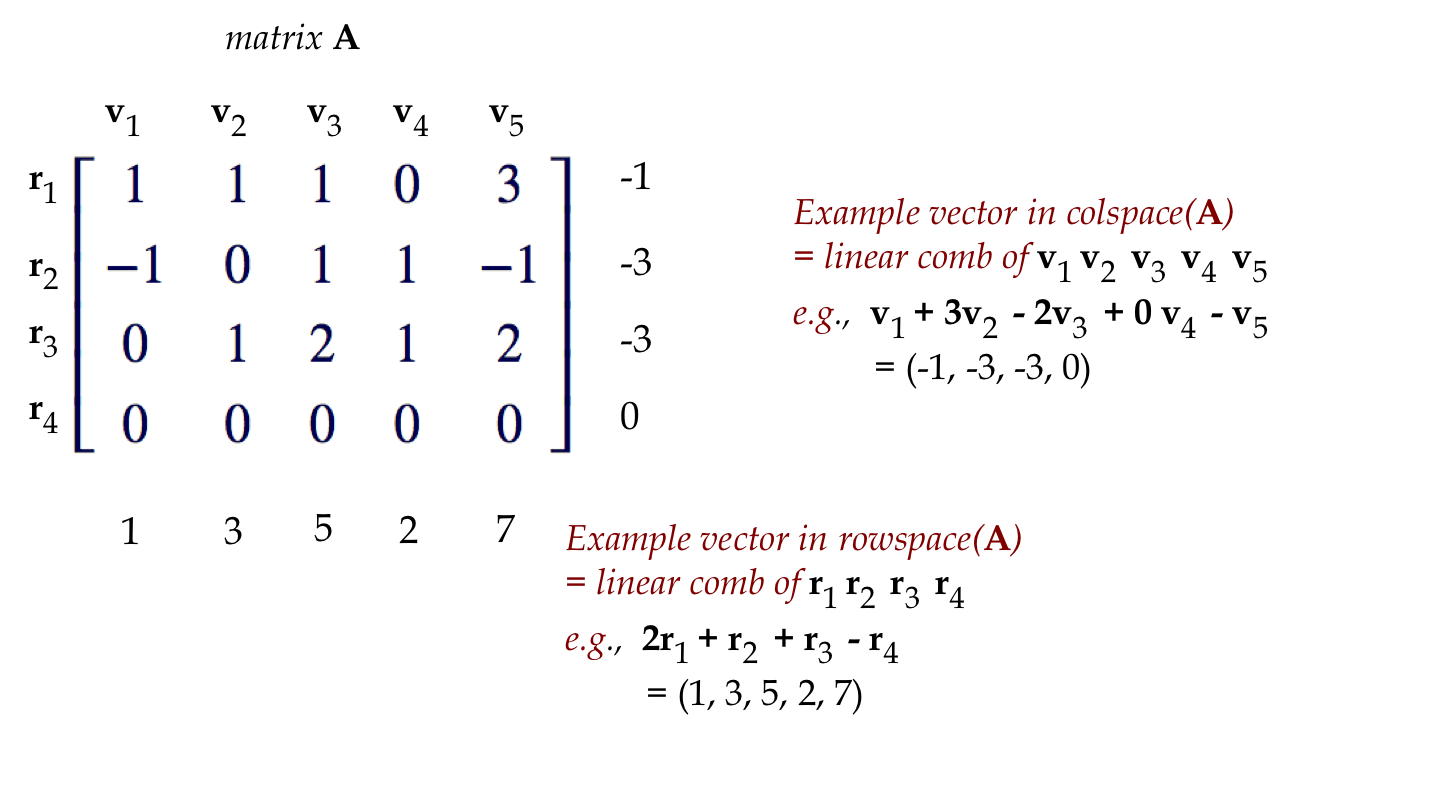
\mat{1 & 1 & 1 & 0 & 3\\
-1 & 0 & 1 & 1 & -1\\
0 & 1 & 2 & 1 & 2\\
0 & 0 & 0 & 0 & 0}
$$
- Here, the rowspace is the set of all vectors that can be
generated by
$$\eqb{
{\bf r}_1 & \eql & (1,1,1,0,3)\\
{\bf r}_2 & \eql & (-1,0,1,1,-1)\\
{\bf r}_3 & \eql & (0,1,2,1,2)
}$$
- Since \({\bf r}_4 = (0,0,0,0,0)\) doesn't add anything
to a linear combination, it's not needed.
- Notice the row space is in 5D (the vectors are 5-dimensional).
- It will turn out that \(\mbox{dim}(\mbox{rowspace}({\bf A}))=2\).
- Thus, even though the vectors are in 5D, fewer are needed
to span the rowspace.
- This is like the 3D examples where two vectors were enough
for the plane.
- The colspace is the span of
$$\eqb{
{\bf c}_1 & \eql & (1,-1,0,0)\\
{\bf c}_2 & \eql & (1,0,1,0)\\
{\bf c}_3 & \eql & (1,1,2,0)\\
{\bf c}_4 & \eql & (0,1,1,0)\\
{\bf c}_5 & \eql & (3,-1,2,0)
}$$
- Here, the colspace is in 4D (the vectors in it are 4-dimensional).
- It will turn out that \(\mbox{dim}(\mbox{colspace}({\bf A}))=2\).
- Thus, even though the vectors are in 4D, fewer are needed
to span the colspace.
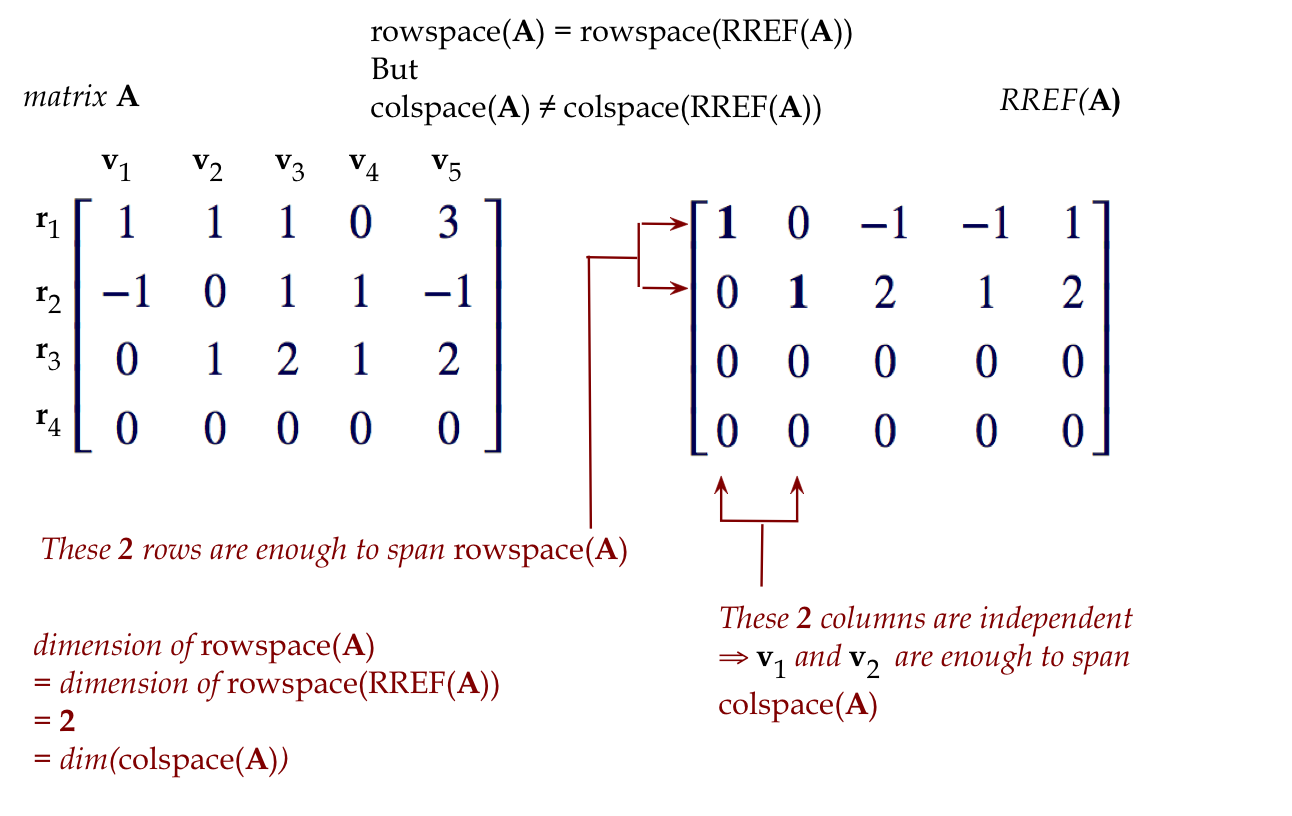
- At this point, it's worth looking at the RREF:
$$
\mat{{\bf 1} & 0 & -1 & -1 & 1\\
0 & {\bf 1} & 2 & 1 & 2\\
0 & 0 & 0 & 0 & 0\\
0 & 0 & 0 & 0 & 0}
$$
-
If you've guessed that the number of pivot rows (which equals the
number of pivot columns) is the dimension, you would be right.
- But we need to prove this.
- An important caution:
- Look at the space spanned by the the pivot columns above.
- It's the plane \((x_1,x_2,0,0)\).
- This is NOT the space spanned by the columns
\({\bf c}_1,\ldots,{\bf c}_5\). For example, the vector
\({\bf c}=(2,1,3,0) = {\bf c}_2 + {\bf c}_3\) is in the colspace
but not in space spanned by the pivot columns.
- However, the dimensions of these two spaces are the
same (equal to 2): meaning, at most two vectors are needed to span.
We will prove Theorem 6.6 in steps:
- First, recall the three row operations in creating an RREF:
- Swapping two rows.
- Scaling a row by a number.
- Adding to a row a scalar multiple of another row.
- Now consider an \(m\times n\) matrix \({\bf A}\) with rows
\({\bf r}_1, \ldots, {\bf r}_m\)
and its rowspace: \(\mbox{span}({\bf r}_1, \ldots, {\bf r}_m)\).
- Suppose we apply a row operation to \({\bf A}\)
and \({\bf A}^\prime\) is the resulting matrix.
In-Class Exercise 15:
Show that the rowspace of \({\bf A}^\prime\) is the
same as the rowspace of \({\bf A}\). Do this for each
of three types of row operations.
- Since the rowspace does not change with row operations,
the rowspace of a matrix \({\bf A}\) is the same as
the rowspace of its RREF.
- That is,
$$
\mbox{rowspace}({\bf A})
\eql
\mbox{rowspace}(RREF({\bf A}))
$$
- Thus
$$
\mbox{dim}(\mbox{rowspace}({\bf A}))
\eql
\mbox{dim}(\mbox{rowspace}(RREF({\bf A})))
$$
- But, in the RREF, only the pivot rows are nonzero.
- And the pivot rows are independent.
In-Class Exercise 16:
Why are the pivot rows independent?
- Thus,
\(\mbox{dim}(\mbox{rowspace}({\bf A}))\) =
the number of pivot rows.
- Now, we know that the number of pivot rows is the same
as the number of pivot columns.
- What we do know is that
$$
\mbox{dim}(\mbox{colspace}(RREF({\bf A})))
\eql \mbox{number of pivot columns}
$$
We also know that
$$
\mbox{colspace}({\bf A})
\; \neq \;
\mbox{colspace}(RREF({\bf A}))
$$
And thus, we cannot (yet) conclude
$$
\mbox{dim}(\mbox{colspace}({\bf A}))
\eql \mbox{number of pivot columns}
$$
- Another way of thinking about this issue:
- We showed that row ops don't change the row space.
- But row ops do change the column space and
so the column space of the matrix is not necessarily the same
as the column space of its RREF.
- What we did show earlier (Proposition 6.3):
$$\mbox{dim}(\mbox{colspace}({\bf A}))
\geq \mbox{dim}(\mbox{colspace}(RREF({\bf A})))
$$
Which means
$$\mbox{dim}(\mbox{colspace}({\bf A}))
\geq \mbox{dim}(\mbox{rowspace}({\bf A}))
$$
Why? Recall:
- The columns of A corresponding to the pivots are independent.
- Thus, the dimension of the colspace is at least that much.
- The number of pivots is the dimension of the rowspace (since
\(\mbox{rowspace}({\bf A})=\mbox{rowspace}(RREF{\bf A})\)).
- To prove the last step, we'll use a really simple,
clever trick.
- For any matrix \({\bf A}\), consider its transpose
\({\bf A}^T\).
- For example:
$$
{\bf A}
\eql
\mat{1 & 1 & 1 & 0 & 3\\
-1 & 0 & 1 & 1 & -1\\
0 & 1 & 2 & 1 & 2\\
0 & 0 & 0 & 0 & 0}
\;\;\;\;\;\;\;\;
{\bf A}^T
\eql
\mat{1 & -1 & 0 & 0\\
1 & 0 & 1 & 0\\
1 & 1 & 2 & 0\\
0 & 1 & 1 & 0\\
3 & -1 & 2 & 0}
$$
- Clearly,
$$\eqb{
\mbox{colspace}({\bf A})
& \eql &
\mbox{rowspace}({\bf A}^T)\\
\mbox{rowspace}({\bf A})
& \eql &
\mbox{colspace}({\bf A}^T)\\
}$$
- So, it must be that
$$
\mbox{dim}(\mbox{colspace}({\bf A}))
\eql
\mbox{dim}(\mbox{rowspace}({\bf A}^T))
\;\; \leq \;\;
\mbox{dim}(\mbox{colspace}({\bf A}^T))
\eql
\mbox{dim}(\mbox{rowspace}({\bf A}))
$$
- So, we have both:
- \( \mbox{dim}(\mbox{rowspace}({\bf A}))
\leq \mbox{dim}(\mbox{colspace}({\bf A})) \)
\(\rhd\)
(via the independence of pivot columns)
- \( \mbox{dim}(\mbox{rowspace}({\bf A}))
\geq \mbox{dim}(\mbox{colspace}({\bf A})) \)
\(\rhd\)
(via the transpose)
- In other words
$$
\mbox{dim}(\mbox{rowspace}({\bf A}))
\eql
\mbox{dim}(\mbox{colspace}({\bf A}))
\bigsp\Box
$$
- Which proves Theorem 6.6.
- The proof of Proposition 6.4 is now trivial because
we've proved something far stronger.
- Let's remind ourselves ...
Proposition 6.4: The rank of the collection
\({\bf v}_1, {\bf v}_2, \ldots, {\bf v}_n\)
is the number of pivot columns of \(RREF({\bf A})\).
In-Class Exercise 17:
Complete the proof of Proposition 6.4.
Finally, let's reinterpret the familiar \({\bf Ax}={\bf b}\):
- Consider this example:
$$
\mat{2 & -3 & 2\\
-2 & 1 & 0\\
1 & 1 & -1}
\vecthree{x_1}{x_2}{x_3}
\eql
\vecthree{5}{-1}{0}
$$
- Written as a linear combination, this is the same as:
$$
x_1 \vecthree{2}{-2}{1} \plss
x_2 \vecthree{-3}{1}{1} \plss
x_3 \vecthree{2}{0}{-1} \eql
\vecthree{5}{-1}{0}
$$
- Suppose we call the column vectors \({\bf v}_1, {\bf v}_2,
{\bf v}_3\):
$$
{\bf v}_1 \eql \vecthree{2}{-2}{1}
\;\;\;\;\;\;\;\;
{\bf v}_2 \eql \vecthree{-3}{1}{1}
\;\;\;\;\;\;\;\;
{\bf v}_3 \eql \vecthree{2}{0}{-1}
$$
- Thus, the question
Is there an \({\bf x}=(x_1,x_2,x_3)\) such that \({\bf Ax}={\bf b}\)?
is the same as the question
Are there scalars \(x_1,x_2,x_3\) such that
\({\bf b} = x_1{\bf v}_1 + x_2{\bf v}_2 + x_3{\bf v}_3\)?
- That is, is \({\bf b} \in \mbox{colspace}({\bf A})\)?
- If there's no solution, the vector
\({\bf b} \notin \mbox{colspace}({\bf A})\).
In-Class Exercise 18:
Prove or disprove the following. Suppose
\({\bf v}_1, {\bf v}_2, \ldots, {\bf v}_n\)
is a collection of \(m\)-dimensional
linearly independent vectors and
\({\bf u} \in \mbox{span}({\bf v}_1, {\bf v}_2, \ldots, {\bf v}_n)\).
Then there is exactly one linear combination of
\({\bf v}_1, {\bf v}_2, \ldots, {\bf v}_n\)
that will produce \({\bf u}\). Consider
both cases, \(m=n\) and \(m\neq n\).
6.5
Basis
We've encountered this idea before, but let's revisit:
Computing a basis:
- Suppose we are given any collection of vectors, not necessarily
independent, and we want to compute a basis of the space spanned
by the vectors.
- That is, suppose we are given vectors
\({\bf v}_1, {\bf v}_2, \ldots, {\bf v}_n\).
- Define the span as
$$
{\bf W} \eql
\mbox{span} ({\bf v}_1, {\bf v}_2, \ldots, {\bf v}_n)
$$
- We'd like a basis for the subspace \({\bf W}\).
- Based on what we now know about the rowspace and colspace,
there are two different ways of identifying a basis
for \({\bf W}\).
- Method 1: use rows
- Create a matrix \({\bf A}\)
with \({\bf v}_1, {\bf v}_2, \ldots, {\bf v}_n\)
as its rows.
- Compute \(RREF({\bf A})\).
- The pivot rows form a basis for the space.
- Why does this work?
- The rowspace is exactly \({\bf W}\) by design.
- The pivot rows span the rowspace.
\(\rhd\)
No more vectors are needed.
- The dimension of the rowspace is the number of pivot rows
\(\rhd\)
At least that many vectors are needed.
- Note: the basis so produced might have no vectors in common with
the set \({\bf v}_1, {\bf v}_2, \ldots, {\bf v}_n\).
- Method 2: use columns
- Create a matrix \({\bf A}\)
with \({\bf v}_1, {\bf v}_2, \ldots, {\bf v}_n\)
as its columns.
- Compute \(RREF({\bf A})\).
- The original columns corresponding to the
pivot columns form a basis for the colspace.
- Why does this work?
- The colspace is exactly \({\bf W}\) by design.
- Suppose there are \(k\) pivot columns are \(i_1, i_2,
\ldots, i_k\).
- Proposition 6.3 showed that
\({\bf v}_{i_1}, {\bf v}_{i_2}, \ldots, {\bf v}_{i_k}\)
are independent.
- Theorem 6.6 showed that \(\mbox{dim}({\bf W}) = k\).
- So, no smaller basis is possible.
- One advantage of the column method is that the basis is
formed from a subset of \({\bf v}_1, {\bf v}_2, \ldots, {\bf v}_n\).
Note the difference between rows and columns:
- For rows:
- The rowspace of the original matrix \({\bf A}\) is the same as the
rowspace of the \(RREF({\bf A})\).
- That is, any vector that's a linear combination of the
rows of \({\bf A}\) is also a linear combination (different scalars)
of the rows of \(RREF({\bf A})\).
- This is not true for columns, as we've seen:
- The colspace of \({\bf A}\) is not necessarily the
the colspace of \(RREF({\bf A})\).
Let's connect dimension and basis directly:
- Recall, for a subspace \({\bf W}\)
- \(\mbox{dim}({\bf W})\) is the minimum number of vectors
needed to span \({\bf W}\).
- A basis is one such minimum collection.
- Thus, the size of a basis is the dimension.
- Are the vectors in a basis independent?
- Proposition 6.7: The vectors in a basis are linearly
independent.
Proof:
If \({\bf u}_1, {\bf u}_2, \ldots, {\bf u}_n\) form a basis
for subspace \({\bf W}\) but are not all linearly independent,
then it is possible to express some \({\bf u}_j\) in terms
of the others, as in
$$
{\bf u}_j \eql \beta_1 {\bf u}_1 + \ldots + \beta_{j-1}{\bf u}_{j_1}
+ \beta_{j+1}{\bf u}_{j+1} + \ldots + \beta_n{\bf u}_n
$$
Since \({\bf u}_1, {\bf u}_2, \ldots, {\bf u}_n\) form a basis,
any \({\bf w} \in {\bf W}\) can be expressed in terms of
these vectors, as in:
$$
{\bf w} \eql \alpha_1 {\bf u}_1 + \ldots + \alpha_{j-1}{\bf u}_{j_1}
+ \alpha_j{\bf u}_j
+ \alpha_{j+1}{\bf u}_{j+1} + \ldots + \alpha_n{\bf u}_n
$$
Substituting for \({\bf u}_j\):
$$\eqb{
{\bf w} & \eql & \alpha_1 {\bf u}_1 + \ldots
+ \alpha_{j-1}{\bf u}_{j-1} +
(\beta_1 {\bf u}_1 + \ldots + \beta_{j-1}{\bf u}_{j_1}
+ \beta_{j+1}{\bf u}_{j+1} + \ldots + \beta_n{\bf u}_n)
+ \alpha_{j+1}{\bf u}_{j+1} + \ldots + \alpha_n{\bf u}_n\\
& \eql &
(\alpha_1+\beta_1) {\bf u}_1 + \ldots
+ (\alpha_{j-1}+\beta_{j-1}){\bf u}_{j-1}
+ (\alpha_{j+1}+\beta_{j+1}){\bf u}_{j+1}
+ \ldots + (\alpha_n + \beta_n){\bf u}_n\\
& \eql &
\gamma_1 {\bf u}_1 + \ldots
+ \gamma_{j-1}{\bf u}_{j-1}
+ \gamma_{j+1}{\bf u}_{j+1}
+ \ldots + \gamma_n {\bf u}_n\\
& \eql &
\mbox{ a linear combination of } {\bf u}_1 + \ldots + {\bf u}_{j-1}
+ {\bf u}_{j+1} + \ldots + {\bf u}_{n}
}$$
with coefficients \(\gamma_i \defn (\alpha_i + \beta_i)\).
That is, we've found a smaller set of vectors that spans \({\bf W}\),
a contradiction. \(\Box\)
6.6
Orthogonality and linear independence
Recall what it means for two vectors to be orthogonal:
- Vectors \({\bf u}\) and \({\bf v}\) are orthogonal if
\({\bf u} \cdot {\bf v} = 0\).
\(\rhd\)
The dot-product is zero.
- The intuition?
- The angle between \({\bf u}\) and \({\bf v}\) is
$$
\cos(\theta)
\eql
\frac{{\bf v} \cdot {\bf u}}{
|{\bf v}| |{\bf u}|}
$$
- Which is zero if \({\bf u} \cdot {\bf v} = 0\).
Orthogonal vectors are linearly independent:
- Proposition 6.8: If \({\bf v}_1, {\bf v}_2, \ldots, {\bf
v}_n\) are pairwise orthogonal, they are linearly independent.
In-Class Exercise 20:
Prove this result:
- Apply the definition of linear independence to
\({\bf v}_1, {\bf v}_2, \ldots, {\bf v}_n\).
- Then compute the dot product with \({\bf v}_1\) on both sides.
- What does this imply for the value of \(\alpha_1\)?
- Complete the proof.
In-Class Exercise 21:
Does the same proof work for complex vectors? Recall that
the dot-product for complex vectors is a bit different.
If the proof fails, why does it fail? If the proof works, explain
all the steps in terms of complex vectors.
6.7
Summary and study tips
Let's summarize a few key points in this module:
- In this module, we developed a bit of the theory of linear
algebra.
- Spaces (or subspaces), span, rank, dimension,
and basis are key concepts in linear algebra.
- Although the concepts are usually defined for collections
of vectors, they're all related through matrices and their RREFs.
- First consider linear independence (LI):
- Informally, if
$$
{\bf v}_2 \eql 3 {\bf v}_1 + 4 {\bf v}_3?
$$
then \({\bf v}_2\) is a linear combination of \({\bf v}_1\) and \({\bf v}_3\).
and therefore, they aren't independent.
- Formally, nonzero vectors \(({\bf v}_1, {\bf v}_2, \ldots, {\bf v}_n\)
are independent if the only solution to the equation
$$
\alpha_1 {\bf v}_1 + \alpha_2 {\bf v}_2 + \ldots + \alpha_n {\bf v}_n
\eql {\bf 0}
$$
is \(\alpha_1 = \alpha_2 = \ldots = \alpha_n = 0\).
- Or in matrix form (with the vectors as columns):
$$
\mat{
& & & \\
\vdots & \vdots & \ldots & \vdots \\
{\bf v}_1 & {\bf v}_2 & \ldots & {\bf v}_n\\
\vdots & \vdots & \ldots & \vdots \\
& & &
}
\mat{\alpha_1\\
\alpha_2\\
\alpha_3\\
\vdots\\
\alpha_n}
\eql
\mat{0\\ 0\\ 0\\ \vdots\\ 0}
$$
implies \({\bf \alpha} = {\bf 0}\)
- Which is true only when the RREF is full-rank.
- Let's look at an example of dependence.
- Consider the vectors
$$
{\bf v}_1 \eql \vecfour{1}{-1}{0}{0}
\;\;\;\;\;\;\;\;\;
{\bf v}_2 \eql \vecfour{1}{0}{1}{0}
\;\;\;\;\;\;\;\;\;
{\bf v}_3 \eql \vecfour{1}{1}{2}{0}
\;\;\;\;\;\;\;\;\;
{\bf v}_4 \eql \vecfour{0}{1}{1}{0}
\;\;\;\;\;\;\;\;\;
{\bf v}_5 \eql \vecfour{3}{-1}{2}{0}
$$
- Put them into matrix \({\bf A}\) as columns and compute \(RREF({\bf A})\):

- The span of a collection of vectors is all the
vectors you get as linear combinations of them:
$$\mbox{span}({\bf u},{\bf v}) \eql \{ {\bf w}: {\bf w}= \alpha{\bf u} +
\beta{\bf v} \}$$
- Consider: the rowspace (span of rows)
and colspace (span of columns) via our example:
- What does this have to do with the RREF?
- Lastly, an important result: any collection of
orthogonal vectors is linearly independent.
- The most important concepts with practical value are:
rank, linear-independence, basis, and what happens as a result of orthogonality.
- The others (subspace, dimension) are useful in the theory.
Study tips:
- This module has both many concepts and theoretical results.
- Remember: one of the best ways
to help grapple with theoretical results is to
try and write your own example that might illustrate
each theoretical result.