Module objectives
By the end of this module, you should be able to
- Explain how matrices achieve geometric transformations such
as reflection and rotation.
- Explain the approach to handling translation via matrices.
- Describe what a basis means.
- Derive matrix-based geometric transformations.
- Derive 3D to 2D transformations.
4.0
A few examples and some questions they raise
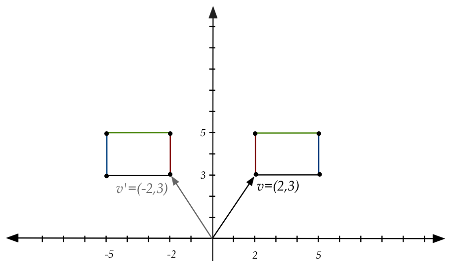
In-Class Exercise 1:
On a piece of paper, draw the points \((2,3), (5,3), (5,5)\)
and \((2,5)\) and join the dots to get a shape. Now, treating each
of these tuples as a 2D vector, multiply each separately by
the matrix \({\bf A}=\mat{-1 & 0\\0 & 1}\) to get four new
vectors. Draw the "points" (heads) corresponding to these
vectors. What is the geometric relationship between
the two shapes?
In-Class Exercise 2:
Download GeomTransExample.java
and MatrixTool.java,
and add your matrix-vector multiplication code from earlier
to MatrixTool. Then, confirm
your calculations above.
You will also need
DrawTool.java.
In-Class Exercise 3:
What matrix would resulting in reflecting a shape about the x-axis?
Note:
- Recall: multiplying a vector by a matrix (the matrix is on the
left) produces another vector.
- In notation: \({\bf Av} = {\bf v}^\prime\) where
\({\bf v}^\prime\) is the transformed vector.
- To transform a line-segment shape:
- Treat each point as a vector.
- Multiply by the "transformation" matrix.
- Join the dots.
- For example:
In-Class Exercise 4:
On paper, draw the same rectangle
(the points \((2,3), (5,3), (5,5), (2,5)\))
and reflect the rectangle about the origin. Use guesswork
to derive the matrix
that will achieve this transformation. Apply the matrix
(call this matrix \({\bf B}\)) to the four corners to verify.
In-Class Exercise 5:
Download GeomTransExample2.java,
and modify the matrix \({\bf B}\) in the code
to achieve reflection about the origin,
and confirm your calculations above.
In-Class Exercise 6:
Download GeomTransExample3.java,
and insert the entries from the
\({\bf A}\) and \({\bf B}\) matrices from above. Work out the
product \({\bf BA}\) by hand and apply to the four corners
of the rectangle to
confirm what the program produces. Argue that the resulting
matrix is intuitively what one would expect.
Applying transformations in sequence:
- When transformations are represented by matrices, the
product applies them in sequence.
- Consider \(5\) transformations in sequence applied to a
vector \({\bf v}\).
- Suppose the i-th transformation is represented by
the matrix \({\bf A}_i\).
- Then suppose the desired sequence is: first apply
\({\bf A}_1\), then apply \({\bf A}_2\), etc.
- The correct multiplication order is:
$$
{\bf A}_5 ({\bf A}_4 ({\bf A}_3 ({\bf A}_2 ({\bf A}_1 {\bf v}))))
$$
- We've already seen earlier that for two matrices
$$
{\bf A}_2 ({\bf A}_1 {\bf v})
\eql
({\bf A}_2 {\bf A}_1) {\bf v}
$$
That is, we can multiply the matrices first to get a single
matrix and then apply the resulting matrix to \({\bf v}\).
- This raises several questions.
- Question 1: Can we multiply out all the matrices and apply the single
resulting matrix to the vector and get the same result?
- Question 2: Is it permissible to do something like this?
- Compute the product \({\bf B} = {\bf A}_4 {\bf A}_3\)
and substitute this:
$$
{\bf A}_5 ({\bf B} ({\bf A}_2 ({\bf A}_1 {\bf v})))
$$
In-Class Exercise 7:
What theoretical property of multiplication do we need to be true
for matrices to resolve questions 1 and 2 above?
In-Class Exercise 8:
In your earlier program,
GeomTransExample3.java,
change the matrix multiplication order from
the product \({\bf BA}\) to the product \({\bf AB}\).
What do you see? Does the order matter?
Confirm by hand calculation.
Is there a geometric reason to expect the result?
What do you conclude about whether matrix multiplication is
commutative?
Now let's try a different type of transformation.
In-Class Exercise 9:
Download
GeomTransExample4.java,
compile and execute.
How would you describe the transformation?
In-Class Exercise 10:
Now, let's apply the earlier reflection about y-axis and
the transformation above in sequence.
In GeomTransExample4.java,
first apply \({\bf AC}\) and then change
to the order to \({\bf CA}\).
What do you see? Does the order matter?
Is there a geometric reason to expect the result?
In-Class Exercise 11:
Download
GeomTransExample5.java,
compile and execute.
Observe that we apply two transformations in sequence: first,
the matrix \({\bf A}\) from above, and then a new matrix \({\bf B}\).
What is the net effect in transforming the rectangle? From that,
can you conclude what matrix \({\bf B}\) would achieve when
applied by itself to a vector?
What is the product matrix \({\bf C}= {\bf BA}\) when printed out?
Consider the generic vector \({\bf v}=(v_1,v_2)\) and
compute by hand the product \({\bf C v}\).
All of the above explorations raise a bunch of questions:
- Why are some matrix multiplications commutative?
- In what ways is matrix multiplication different from regular
number multiplication?
- How does one design a matrix for a desired transformation?
- How does one compute the "reverse" of a matrix?
- Which matrices result in no change to a vector? Is this
true only for some vectors?
Let's start with matrix multiplication properties
4.1
Properties of matrix multiplication
The following are generally useful properties:
- First, a non-property: matrix multiplication is, alas, NOT commutative:
that is, in general,
$$
{\bf A B} \;\; \neq \;\; {\bf B A}
$$
- Matrix multiplication is associative:
$$
{\bf A (B C)} \eql {\bf (A B) C}
$$
- Matrix multiplication distributes over matrix addition:
$$
{\bf A (B + C)} \eql {\bf (A B) + (A C)}
$$
- Scalar multiplication can be applied in any order:
$$
\alpha {\bf (A B)} \eql {\bf (\alpha A) B}
\eql {\bf A (\alpha B)}
$$
In-Class Exercise 12:
Prove the above properties.
In-Class Exercise 13:
Do the properties above directly imply that
\(
{\bf (A + B) C} \eql {\bf (A C) + (B C)}?
\)
Or is a separate proof needed?
4.2
Two key ideas: span and basis
Let's start with span:
- Consider a linear combination of two vectors:
\({\bf w} = \alpha{\bf u} + \beta{\bf v}\)
- Example:
- The question arises: for a given pair \({\bf u,v}\),
is it true that every possible \({\bf w}\) can be expressed
as a linear combination of \({\bf u}\) and \({\bf v}\)?
- That is, does there exist a \({\bf w}^\prime\) for which we cannot
find \(\alpha,\beta\) such that \({\bf w}^\prime = \alpha{\bf u} + \beta{\bf v}\)?
- We'll consider the opposite:
what is the set of vectors that can
be expressed as a linear combination of \({\bf u,v}\)?
- We will define span\(({\bf u,v}) = \{{\bf w}:
\exists \alpha,\beta \mbox{ such that }
{\bf w} = \alpha{\bf u} + \beta{\bf v}\}\).
- Read the first part of the right side as "set of all \({\bf w}\)
such that there exist \(\alpha,\beta\) ..."
- The colon after \({\bf w}:\) is "such that"
- \(\exists\) is short for "there exists" or "there exist"
- In general, for \(n\) dimensions:
Definition: the span of a collection of vectors
\({\bf u}_1, {\bf u}_2, \ldots, {\bf u}_k\) is the set
of vectors expressible as a linear combination of the
\({\bf u}_i\)'s, i.e.,
$$
span({\bf u}_1, {\bf u}_2, \ldots, {\bf u}_k)
\eql
\{{\bf w}: \exists \alpha_1,\ldots,\alpha_k \mbox{ such that }
{\bf w} = \alpha_1{\bf u}_1 + \ldots + \alpha_k{\bf u}_k\}.
$$
In-Class Exercise 14:
To explore this notion, write code in
ExploreSpan.java to
compute a linear combination. Observe the systematic exploration
of different values of \(\alpha,\beta\). Change the range
to see if you can "fill up" the space.
In-Class Exercise 15:
What's an example of vectors \({\bf u,v}\) whose span is
not the whole space of 2D vectors?
Similarly, what's an example of 3D vectors \({\bf u}_1,{\bf u}_2,{\bf u}_3\),
whose span is not the whole space of 3D vectors?
In-Class Exercise 16:
Is there a pair of 3D vectors that spans the whole space of 3D
vectors?
Next, let's examine the idea of a basis:
Definition:
A basis is a minimal set (as few as possible)
of vectors that span a given space.
- Example: we suspect that \({\bf u}=(1,4), {\bf v}=(2,3)\)
span 2D space and just one of them alone is not enough.
- We will later prove that \(n\) vectors are both needed
and sufficient to span \(n\)-dimensional space.
In-Class Exercise 17:
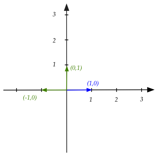
Consider the pair of "special" vectors
\({\bf e}_1=(1,0), {\bf e}_2=(0,1)\).
- Express the vector \((1,4)\) as a linear combination of
\({\bf e}_1, {\bf e}_2\).
- Express the vector \((2,3)\) as a linear combination of
\({\bf e}_1, {\bf e}_2\).
- Do \({\bf e}_1, {\bf e}_2\) span 2D space?
- What are the corresponding three "special" vectors that span 3D space?
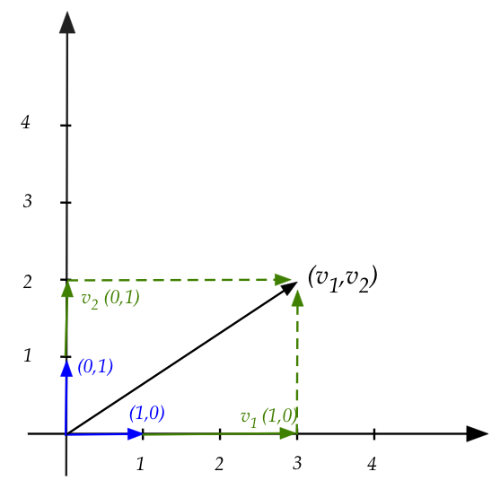
Coordinates:
- The basis formed with vectors \({\bf e}_i\) above is called the
standard basis.
- We see that the scalars used with the standard basis
turn out to be the coordinates of the target vector's
arrowhead.
- Example:
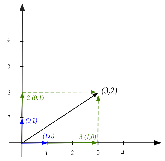
- Each basis vector is multiplied by a scalar.
- \(3{\bf e}_1 = 3(1,0) = (3,0)\)
- \(2{\bf e}_2 = 2(0,1) = (0,2)\)
- The scaled vectors are added to get \((3,2)\):
$$ (3,0) + (0,2) = (3,2) $$
- Another example:
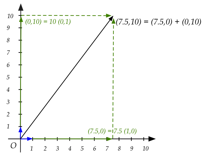
We will broaden the idea of coordinates as follows:
- Any time a basis is used to express a vector (via linear combination),
the scalars form the coordinates of that vector
with respect to the given basis.
- So, if that's the case, can a vector have coordinates in
non-standard basis?
- Let's assume that \({\bf u}=(1,4)\) and
\({\bf v}=(3,2)\) form a basis.
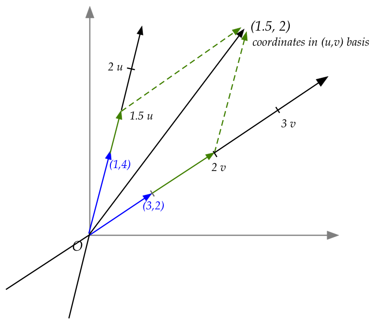
- We see that potential scalar multplications of \({\bf u}\)
form a \({\bf u}\)-axis.
- Likewise, there's an implied \({\bf v}\)-axis
- Just like our standard axes, we can imagine integer
multiples of the basis vectors forming "ticks" along
these axes.
- The actual multiples that add up to the result form
the coordinates along these axes.
- Did it feel weird that the first axis (\({\bf u}\)-axis)
is "above" the second one \({\bf v}\)-axis?
- We see that there's no inherent need to have our
standard horizontal axis be the first coordinate.
- It's just convention.
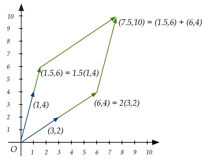
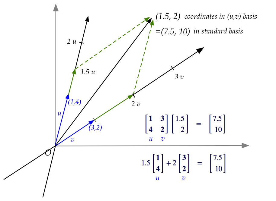
Let's now write the same linear combinations in matrix form:
- The linear combination of vectors:
$$
{\bf 1.5} \vectwo{1}{4} + {\bf 2} \vectwo{3}{2}
\eql
\vectwo{7.5}{10}
$$
is written in matrix form (this is the definition of a matrix,
after all) as:
$$
\mat{1 & 3\\ 4 & 2}
\vectwo{\bf 1.5}{\bf 2}
\eql
\vectwo{7.5}{10}
$$
- We can now look at \((1.5,2)\) as a vector:
- Then it appears that \((1.5,2)\) is being transformed
to \((7.5,10)\).
- Here, one can think of \((1.5,2)\) as a vector
in the "non-standard world".
- And so, when the matrix \(\mat{1 & 3\\ 4 & 2}\) is applied
to it, we think of the vector \((1.5,2)\) (in "non-standard world")
being transformed to \((7.5,10)\) (in "standard world").
- Now let's get back to the matrix:
$$
\mat{{\bf 1} & {\bf 3}\\ {\bf 4} & {\bf 2}}
\vectwo{1.5}{2}
\eql
\vectwo{7.5}{10}
$$
- Each of the columns
of the matrix \(\mat{1 & 3\\ 4 & 2}\)
is a vector in the basis formed by \({\bf u}=(1,4)\) and
\({\bf v}=(3,2)\).
- That is, the columns of a matrix that transforms
are vectors of some basis.
- We'll call the matrix a "basis matrix", when we need
to emphasize this.
- Now for a critical observation:
- When we interpret the matrix-vector multiplication (on the left)
$$
\mat{{\bf 1} & {\bf 3}\\ {\bf 4} & {\bf 2}}
\vectwo{1.5}{2}
\eql
\vectwo{7.5}{10}
$$
as the linear combination
$$
1.5 \vectwo{\bf 1}{\bf 4} + 2 \vectwo{\bf 3}{\bf 2}
\eql
\vectwo{7.5}{10}
$$
then \(1.5,2\) are coordinates in \({\bf u,v}\)-world.
- Notice also that the basis vectors of \({\bf u,v}\)-world
are expressed in standard-world coordinates.
- Thus, the effect of matrix multiplication can be
summarized as
$$
\mat{\mbox{matrix with columns that are}\\
\mbox{basis vectors in another world}\\
\mbox{expressed in standard coords}}
\times
\mat{\mbox{coords of}\\
\mbox{vector in}\\
\mbox{that world}}
\eql
\mat{\mbox{coords of}\\
\mbox{same vector in}\\
\mbox{standard world}}
$$
- Thus, a matrix multiplication can be interpreted as a
change of coordinates from one world to another.
- We will use this observation to design matrices
to achieve the transformations we want (rotation, reflection etc).
4.3
Understanding how to build your own transforms
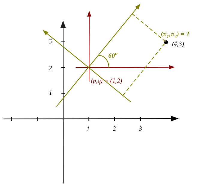
Let's start with an example:
- Suppose we want to rotate the vector \((4,3)\) by \(60^\circ\):
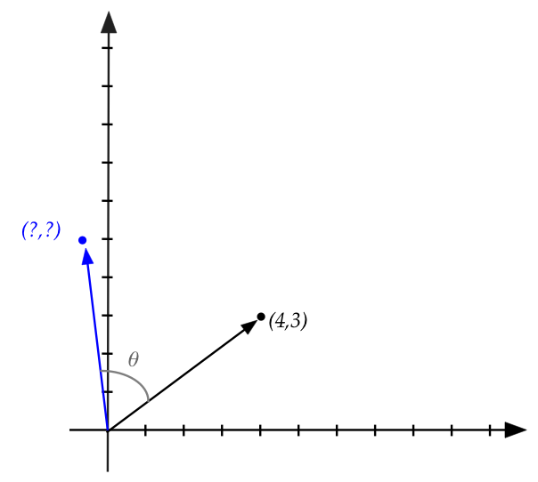
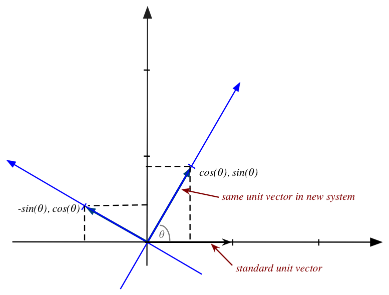
- The first step is to imagine rotating the standard axes
by \(60^\circ\):
Then, in the rotated axes, the rotated point has the same coordinates \((4,3)\)
in the rotated coordinate system.
- It is this new point, the point that has coordinates
\((4,3)\) in the rotated system, whose standard coordinates
we seek.
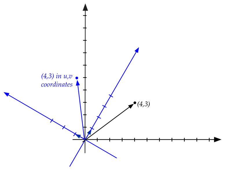
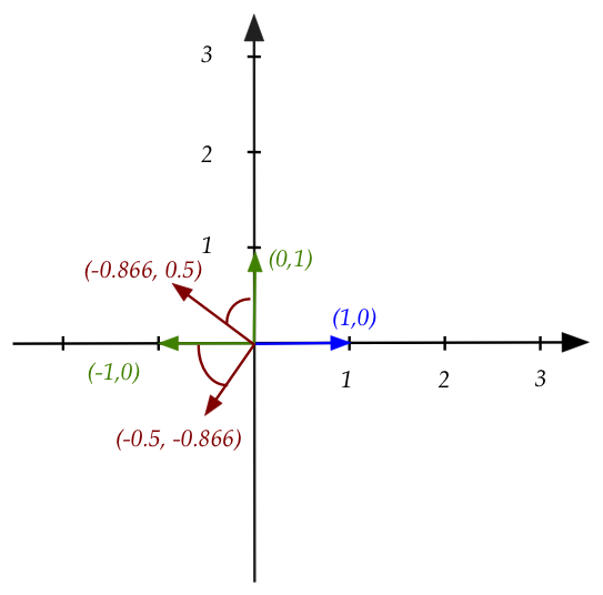
- We will do this by finding the coordinates of the basis
vectors of the rotated system, expressed in the standard coordinates
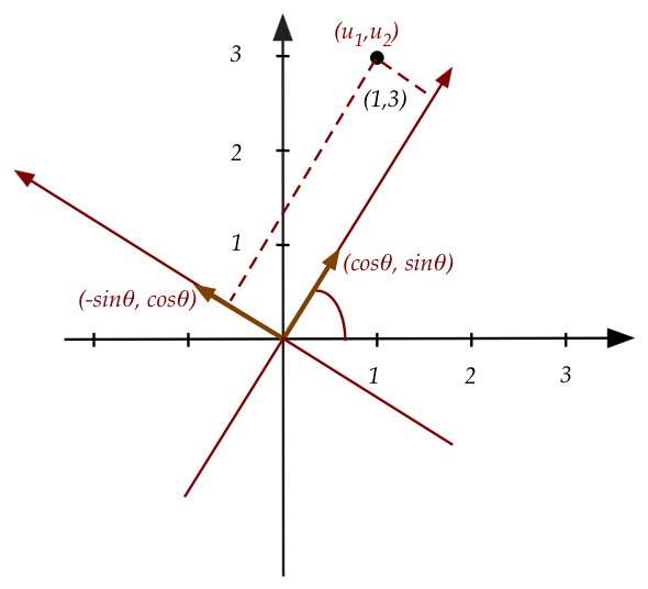
(shown larger here):
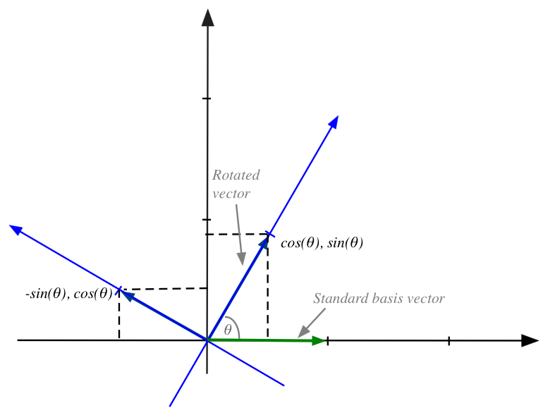
- The first basis vector is \((1,0)\) (in rotated world coordinates)
\(\rhd\)
This becomes \((\cos(\theta), \sin(\theta))\) in standard coordinates.
- The second basis vector is \((0,1)\) (in rotated world coordinates)
\(\rhd\)
This becomes \((-\sin(\theta), \cos(\theta))\) in standard coordinates.
In-Class Exercise 18:
Explain why this is so. That is, why do we get
\((\cos(\theta), \sin(\theta)\) and
\((-\sin(\theta), \cos(\theta))\)?
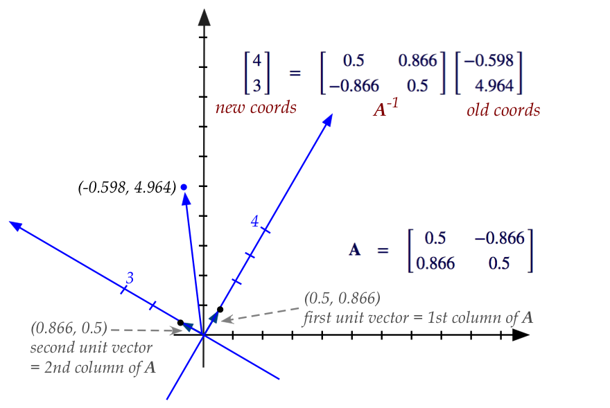
- We can now write the matrix using the basis vectors
(expressed in standard coordinates)
$$
\mat{\cos(\theta) & -\sin(\theta)\\
\sin(\theta) & \cos(\theta)}
$$
- We can now apply this to any vector like \((4,3)\):
$$
\mat{\cos(\theta) & -\sin(\theta)\\
\sin(\theta) & \cos(\theta)}
\vectwo{4}{3}
$$
- What does "apply" mean here? It merely means that
\(4\) and \(3\) are the scalars in the linear combination:
$$
4 \vectwo{\cos(\theta)}{\sin(\theta)}
+
3 \vectwo{-\sin(\theta)}{\cos(\theta)}
$$
- It is this linear combination that gives the
target vector.
\(\rhd\)
And hence the desired coordinates of the transformed vector.
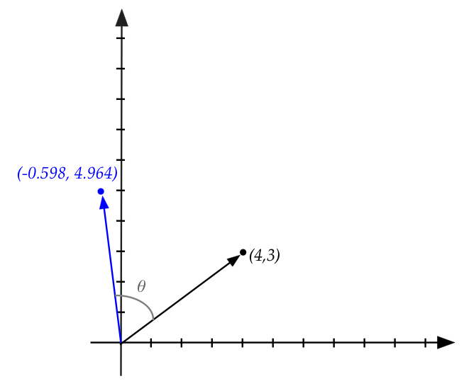
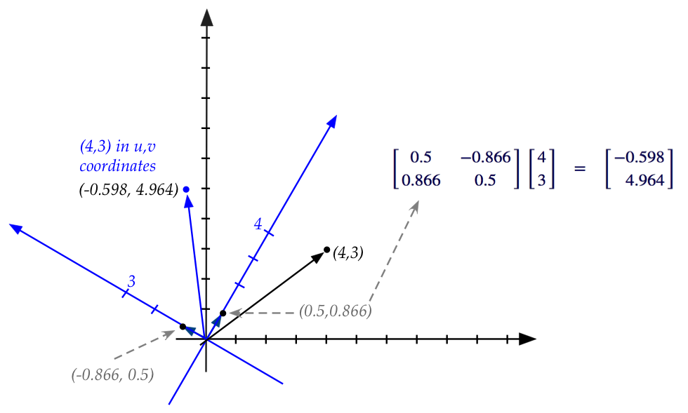
- For example, with \(\theta=60^\circ=\frac{pi}{3}\),
$$
\mat{\cos(\theta) & -\sin(\theta)\\
\sin(\theta) & \cos(\theta)}
\approx
\mat{0.5 & -0.866\\ 0.866 & 0.5}
$$
Thus,
$$
\mat{0.5 & -0.866\\ 0.866 & 0.5}
\vectwo{4}{3}
\eql
\vectwo{-0.598}{4.964}
$$
- Why exactly does this work?
- First, remember that the coordinates \((4,3)\)
in the standard system will be the same coordinates in
rotated system (because those axes are rotated the same way).
- Second, coordinates are nothing but the multipliers (scalars) in
the linear combination of basis vectors (in either system).
- Third, if we express new basis vectors in standard
coordinates, the same linear combination will give us
the standard coordinates of the rotated point.
- Fourth, it is easy to express the new basis vectors in
standard coordinates.
- Fifth, the linear combination is written in matrix form,
with the basis vectors as columns.
- This is why that matrix is the desired transformation matrix
that takes old coordinates into new coordinates.
In-Class Exercise 19:
Use the step-by-step approach above to derive transformation
matrices for:
- Clockwise rotation by \(\theta\).
- Reflection about the x-axis.
In-Class Exercise 20:
What happens when the approach is applied to translation?
That is, suppose we want each point \((x,y)\) to be translated
to \((x+1, y+2)\).
In-Class Exercise 21:
Prove that no matrix multiplication can achieve translation.
That is, no \(2\times 2\) matrix can transform every vector \((x,y)\)
to \((x+p,y+q)\).
4.4
The affine trick (for translation)
We saw earlier that there is no matrix \({\bf A}\) to apply
to every vector \((x,y)\) that will result in the vector
\((x+a,y+b)\).
Now consider this product:
$$
\mat{1 & 0 & p\\
0 & 1 & q\\
0 & 0 & 1}
\vecthree{x}{y}{1}
\eql
\vecthree{x+p}{y+q}{1}
$$
What just happened?
- We've increased the dimension by one (to 3D).
- We included the translation amounts \(p,q\) as the
first two elements of the new third column.
- Each 2D vector \((x,y)\) is extended to the 3D vector
\((x,y,1)\).
- After multiplying, we merely "read off" the translated
coordinates \((x+p,y+q)\) from the 3D vector \((x+p,y+q,1)\).
One concern at this point might be: will such a transformation
work along with the other ones (reflection, rotation)?
In-Class Exercise 22:
Consider some 2D matrix \({\bf C}=\mat{c_{11} & c_{12}\\ c_{21} &
c_{22}}\) applied to a 2D vector \((x,y)\). What is the
resulting vector? What is the result of applying
\(\mat{
c_{11} & c_{12} & 0\\
c_{21} & c_{22} & 0\\
0 & 0 & 1}
\)
to \((x,y,1)\)?
Clearly, the 3D extension, called the affine extension
preserves any 2D transformation.
Let's look at an example:
- Consider anti-clockwise rotation by \(\theta = 60^\circ\).
- The 2D matrix, we saw earlier, was
$$
\mat{\cos(\theta) & -\sin(\theta)\\
\sin(\theta) & \cos(\theta)}
\eql
\mat{0.5 & -0.866\\ 0.866 & 0.5}
$$
- Hence, the affine extension is
$$
\mat{\cos(\theta) & -\sin(\theta) & 0\\
\sin(\theta) & \cos(\theta) & 0\\
0 & 0 & 1}
\eql
\mat{0.5 & -0.866 & 0\\ 0.866 & 0.5 & 0\\ 0 & 0 & 1}
$$
- Next, let's see how this would work in code:
	// Build the entries of the 2D rotation matrix
	double theta = Math.PI/3.0;
	double a11 = Math.cos (theta);
	double a12 = -Math.sin (theta);
	double a21 = Math.sin (theta);
	double a22 = Math.cos (theta);

	// Insert into 3D affine extension:
	double[][] A = {
	    {a11, a12, 0},
	    {a21, a22, 0},
	    {0,   0,   1}
	};

	// Apply to the affine extension of (4,3):
	double[] u = {4,3,1};
	double[] v = matrixVectorMult (A, u);

	// Here, (v[0], v[1]) is the 2D vector.
- We are of course curious about what the 3D vectors look like.
In-Class Exercise 23:
Examine the code in
AffineExample.java,
then compile and execute.
Then, do the same for
Affine3DExample.java.
Move the viewpoint so that you see the (x,y) axes in the usual way
(looking along the z-axis), and compare with the 2D drawing.
Thus, we see that the 2D part of the 3D extension is a
projection (shadow) of the 3D vector onto the (x,y)-plane.
We now need to worry about this: do affine extensions void
the advantages we had with multiplying matrices for
combining transformations?
Let's devise some notation to clarify:
- Let \(\mbox{affine}({\bf A})\) be the \(3\times 3\)
extension of the \(2\times 2\) matrix \({\bf A}\).
- To extract the \(2\times 2\) part from an affine-extended
matrix, let's define
\({\bf A}= \mbox{proj}(\mbox{affine}({\bf A}))\).
- For example:
$$
\mbox{affine}\left(
\mat{0.5 & -0.866 \\ 0.866 & 0.5}
\right)
\eql
\mat{0.5 & -0.866 & 0\\ 0.866 & 0.5 & 0\\ 0 & 0 & 1}
$$
- And
$$
\mbox{proj}\left(
\mat{0.5 & -0.866 & 0\\ 0.866 & 0.5 & 0\\ 0 & 0 & 1}
\right)
\eql
\mat{0.5 & -0.866 \\ 0.866 & 0.5}
$$
- Similarly, for a vector \({\bf u}=(u_1,u_2)\):
- Let \(\mbox{affine}({\bf u}) = (u_1,u_2,1)\)
- Let \(\mbox{proj}(u_1,u_2,*) = (u_1,u_2)\).
- Example: \({\bf u}=(4,3)\)
- \(\mbox{affine}(4,3) = (4,3,1)\)
- \(\mbox{proj}(4,3,1) = (4,3)\)
- So, what's important to know:
given 2D transformations \({\bf A,B}\), is
$$
{\bf B A u}
= \mbox{proj}(
\mbox{affine}({\bf B})
\;\; \mbox{affine}({\bf A}) \;\;\mbox{affine}({\bf u})
)?
$$
- In other words: if we apply affine extensions in sequence
through matrix multiplication and then project, do we get
the same result as we did with matrix multiplication in the
lower dimension?
In-Class Exercise 24:
Show that this is indeed the case.
Whew! This means we can apply rotations, reflections and
translations ad nauseum in sequence through matrix multiplication.
In-Class Exercise 25:
Examine
AffineExample2.java
to see how rotation (by \(60^\circ\)) followed by translation
by \((3,4)\) works via combining the results into a single matrix,
and applying it to the point \((5,1)\). Compile and execute.
It's confusing to see what translation does, so it's best
to draw an arrow from the shifted origin, (\(3,4)\), to the
new coordinates.
4.5
The identity matrix
It's easy to see (3D example) that for
vector \({\bf v}=(v_1,v_2,v_3)\)
$$
\mat{1 & 0 & 0\\
0 & 1 & 0\\
0 & 0 & 1}
\vecthree{v_1}{v_2}{v_3}
\eql
\vecthree{v_1}{v_2}{v_3}
$$
By "cranking out" the multiplication, one can see that this will
be true in \(n\) dimensions:
$$
\mat{1 & 0 & \cdots & 0\\
0 & 1 & \cdots & 0\\
\vdots & \vdots & \vdots & \vdots\\
0 & 0 & \cdots & 1}
\vecdots{v_1}{v_2}{v_n}
\eql
\vecdots{v_1}{v_2}{v_n}
$$
This special matrix, with 1's on the diagonal and
0's everywhere else, is called the identity matrix, often
written as \({\bf I}\)
$$
{\bf I}
\eql
\mat{1 & 0 & \cdots & 0\\
0 & 1 & \cdots & 0\\
\vdots & \vdots & \vdots & \vdots\\
0 & 0 & \cdots & 1}
$$
But there's more to it:
- Recall the special vectors, \((1,0)\) and \((0,1)\)
\(\rhd\)
The standard basis vectors.
- In 3D, for example, the standard basis consists
of the three vectors
\((1,0,0)\), \((0,1,0)\) and \((0,0,1)\)
- In \(n\) dimensions, we would have \(n\) vectors
in the standard basis.
\(\rhd\)
The i-th vector has all zeroes except for a '1' in the
i-th component.
- Let's draw the 2D case:
- Here, we see that for any vector \({\bf v}=(v_1,v_2)\),
multiplication by the identity matrix is really a linear
combination of the standard basis vectors:
$$
\mat{1 & 0\\
0 & 1}
\vectwo{v_1}{v_2}
\eql
v_1 \vectwo{1}{0} + v_2 \vectwo{0}{1}
$$
- Each coordinate \(v_i\) stretches the appropriate basis vector
by the scalar amount \(v_i\)
\(\rhd\)
Which gives \(v_i\) since the basis vector has a '1'.
- Thus, the columns of the identity matrix are really the
standard basis vectors.
Why is it called the identity matrix?
- The term identity is used for an element that does
not change another when an operator is applied.
- The multiplicative identity for integers is the number \(1\)
\(\rhd\)
Multiplying a number \(x\) by \(1\) results in \(x\).
- The additive identity is, obviously, \(0\).
- Since multiplying a vector by \({\bf I}\) leaves the
vector unchanged (i.e., \({\bf I v} = {\bf v}\)),
\({\bf I}\) is called the identity matrix.
- What's interesting: the same matrix is also the identity
for matrices:
$$
{\bf I A} \eql {\bf A}
$$
for any multiply-compatible matrix \({\bf A}\).
In-Class Exercise 26:
Prove the above result. Is it true that \({\bf A I} = {\bf A}\)?
Is it possible to have an identity matrix for an \(m \times n\) matrix?
Clearly, a "crank it out" proof works. But is there a connection
with the interpretation we saw earlier, with the standard basis vectors?
Turns out, there is one. And it leads to a useful perspective
on matrix multiplication in general.
4.6
Matrix multiplication: a different view
Consider the multiplication of two matrices \({\bf A}\) and \({\bf
B}\).
We're going to "unpack" the second matrix:
$$
{\bf A B} \eql
{\bf A}
\mat{b_{11} & b_{12} & \cdots & b_{1n}\\
b_{21} & b_{22} & \cdots & b_{2n}\\
b_{31} & b_{32} & \cdots & b_{3n}\\
\vdots & \vdots & \vdots & \vdots\\
b_{n1} & b_{n2} & \cdots & b_{nn}}
$$
and now name the columns of \({\bf B}\) going left to right
as \({\bf b}_1, {\bf b}_2, \ldots, {\bf b}_n\).
Then,
$$
{\bf A}
\mat{b_{11} & b_{12} & \cdots & b_{1n}\\
b_{21} & b_{22} & \cdots & b_{2n}\\
b_{31} & b_{32} & \cdots & b_{3n}\\
\vdots & \vdots & \vdots & \vdots\\
b_{n1} & b_{n2} & \cdots & b_{nn}
}
\eql
{\bf A}
\mat{ & & & \\
\vdots & \vdots & \vdots & \vdots\\
{\bf b}_1 & {\bf b}_2 & \cdots & {\bf b}_n\\
\vdots & \vdots & \vdots & \vdots\\
& & &
}
$$
Let's now suppose that the result is matrix \({\bf C}\)
with columns named \({\bf c}_1, {\bf c}_2, \ldots, {\bf c}_n\).
So,
$$
{\bf A}
\mat{ & & & \\
\vdots & \vdots & \vdots & \vdots\\
{\bf b}_1 & {\bf b}_2 & \cdots & {\bf b}_n\\
\vdots & \vdots & \vdots & \vdots\\
& & &
}
\eql
\mat{ & & & \\
\vdots & \vdots & \vdots & \vdots\\
{\bf c}_1 & {\bf c}_2 & \cdots & {\bf c}_n\\
\vdots & \vdots & \vdots & \vdots\\
& & &
}
$$
Now for a key observation: \({\bf A} {\bf b}_i = {\bf c}_i\).
In-Class Exercise 27:
Why is this true?
This means that
$$
{\bf A}
\mat{ & & & \\
\vdots & \vdots & \vdots & \vdots\\
{\bf b}_1 & {\bf b}_2 & \cdots & {\bf b}_n\\
\vdots & \vdots & \vdots & \vdots\\
& & &
}
\eql
\mat{ & & & \\
\vdots & \vdots & \vdots & \vdots\\
{\bf A b}_1 & {\bf A b}_2 & \cdots & {\bf A b}_n\\
\vdots & \vdots & \vdots & \vdots\\
& & &
}
$$
In other words, when a matrix \({\bf A}\) multiplies another
matrix \({\bf B}\) the resulting matrix is a concatenation of
multiplying \({\bf A}\) by the columns of \({\bf B}\).
This will be useful in some situations.
Let's see what this means geometrically:
- Consider a reflection about the y-axis followed by a rotation
of \(60^\circ\).
- We've written this before as the product
$$
\mat{\cos(\theta) & -\sin(\theta)\\
\sin(\theta) & \cos(\theta)}
\mat{-1 & 0\\
0 & 1}
\eql
\mat{0.5 & -0.866\\
0.866 & 0.5}
\mat{-1 & 0\\
0 & 1}
$$
- The product happens to equal
$$
\mat{0.5 & -0.866\\
0.866 & 0.5}
\mat{-1 & 0\\
0 & 1}
\eql
\mat{-0.5 & -0.866\\
-0.866 & 0.5}
$$
- But recall that the reflection matrix was derived by
seeing how the basis vectors were changed:
- The original basis vectors are \((1,0)\)
and \((0,1)\).
- The basis vectors of the reflected space are \((-1,0)\)
and \((0,1)\).
- Since the reflected \((0,1)\) is the same as \((0,1)\)
the figure shows the reflected one.
- It is these reflected basis vectors that are rotated:
- Now one can see that the entire rotation matrix applies
to each individual column of the reflection matrix.
- That is,
$$
\mat{0.5 & -0.866\\
0.866 & 0.5}
\vectwo{-1}{0}
\eql
\vectwo{-0.5}{-0.866}
$$
and
$$
\mat{0.5 & -0.866\\
0.866 & 0.5}
\vectwo{0}{1}
\eql
\vectwo{-0.866}{0.5}
$$
- This should make sense because we are rotating each basis
vector.
- To summarize:
- We're looking at the product of two matrices \({\bf A B} =
{\bf C}\).
- If \({\bf B}\)'s columns are vectors of interest, such
as unit vectors, then the product can be interpreted
column-by-column.
- Each column of \({\bf C}\) is a result of applying
the transformation \({\bf A}\) to the corresponding
column of \({\bf B}\).
Let's apply this to a matrix \({\bf A}\) multiplied into the identity
matrix \({\bf I}\), for example, in 2D:
$$
\mat{a_{11} & a_{12}\\ a_{21} & a_{22}}
\mat{ 1 & 0\\ 0 & 1}
$$
- Observe what we get when multiplying into the first column
of the identity matrix:
$$
\mat{a_{11} & a_{12}\\ a_{21} & a_{22}}
\vectwo{1}{0}
\eql
\vectwo{a_{11}}{a_{21}}
$$
That is, we get the first column of \({\bf A}\)
- Similarly, multiplying \({\bf A}\) into the
second column of \({\bf I}\):
$$
\mat{a_{11} & a_{12}\\ a_{21} & a_{22}}
\vectwo{0}{1}
\eql
\vectwo{a_{12}}{a_{22}}
$$
- Thus, we should not be surprised that \({\bf AI}={\bf A}\)
4.7
The reverse of a transformation
For many of the examples seen so far, it's easy to
figure out how to "undo" a transformation:
- Example: rotation by \(60^\circ\):
- The matrix for this rotation is:
$$
\mat{\cos(\frac{\pi}{3}) & -\sin(\frac{\pi}{3})\\
\sin(\frac{\pi}{3}) & \cos(\frac{\pi}{3})}
\eql
\mat{0.5 & -0.866\\
0.866 & 0.5}
$$
- To "undo", we rotate by \(-60^\circ\):
$$
\mat{\cos(-\frac{\pi}{3}) & -\sin(-\frac{\pi}{3})\\
\sin(-\frac{\pi}{3}) & \cos(-\frac{\pi}{3})}
\eql
\mat{0.5 & 0.866\\
-0.866 & 0.5}
$$
In-Class Exercise 28:
What is the "undo" matrix for the reflection about the y-axis?
Multiply the undo matrix (on the left) and the original.
4.8
Change of coordinate frame
Another interpretation of a transformation is that it
changes the coordinate frame.
For example, consider rotating the axes by \(60^\circ\):
- Consider the point \((1,3)\) in the standard frame.
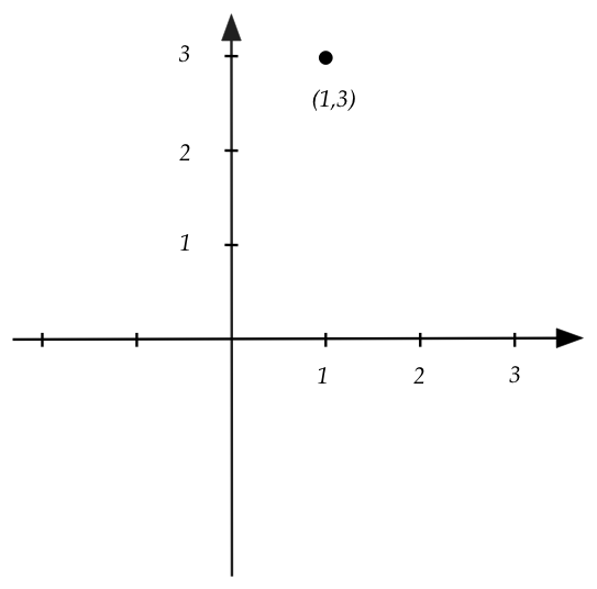
- We now consider an alternate frame whose axes
happen to be rotated by \(60^\circ\):
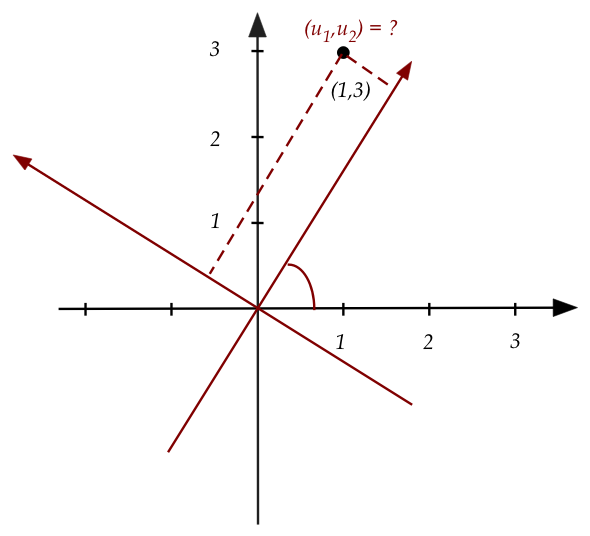
- We would like the coordinates of the point
\((1,3)\) in the new frame.
- Let \({\bf u}=(u_1,u_2)\) be the coordinates in the
second frame.
- We know that the coordinates \((u_1,u_2)\) are
"stretches" of the basis vectors in that frame.
- These basis vectors, we've calculated before, are the
columns of:
$$
\mat{\cos(\theta) & -\sin(\theta)\\
\sin(\theta) & \cos(\theta)}
$$
- Thus, using \(u_1,u_2\) as scalars in a linear combination
of the basis vectors will give us the old coordinates \((1,3)\):
$$
\mat{\cos(\theta) & -\sin(\theta)\\
\sin(\theta) & \cos(\theta)}
\vectwo{u_1}{u_2}
\eql
\vectwo{1}{3}
$$
- Now multiply both sides by the inverse of the matrix, which
is the matrix that rotates \(-60^\circ\):
$$
\mat{\cos(\theta) & \sin(\theta)\\
-\sin(\theta) & \cos(\theta)}
\mat{\cos(\theta) & -\sin(\theta)\\
\sin(\theta) & \cos(\theta)}
\vectwo{u_1}{u_2}
\eql
\mat{\cos(\theta) & \sin(\theta)\\
-\sin(\theta) & \cos(\theta)}
\vectwo{1}{3}
$$
Which simpifies to:
$$
\mat{1 & 0\\
0 & 1}
\vectwo{u_1}{u_2}
\eql
\mat{\cos(\theta) & \sin(\theta)\\
-\sin(\theta) & \cos(\theta)}
\vectwo{1}{3}
$$
Which means
$$
\vectwo{u_1}{u_2}
\eql
\mat{\cos(\theta) & \sin(\theta)\\
-\sin(\theta) & \cos(\theta)}
\vectwo{1}{3}
$$
Which, when \(\theta=60^\circ\), results in
$$
\vectwo{u_1}{u_2}
\eql
\mat{0.5 & 0.866\\
-0.866 & 0.5}
\vectwo{1}{3}
\eql
\vectwo{3.098}{0.634}
$$
- To summarize:
- Derive the matrix that expresses the new frame's unit vectors in the
current frame.
- Find the inverse.
- Apply the inverse to the old coordinates to get the new one.
- Sample implementation:
CoordChange.java
A translation example:
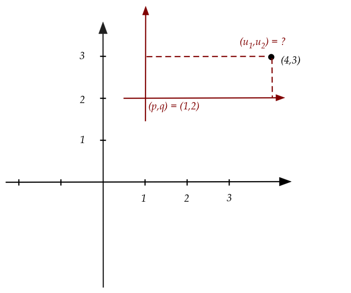
Suppose the new axes are translated by \((1,2)\).
In-Class Exercise 30:
Follow the steps to compute the affine-extended matrix that, when applied
to the point \((4,3)\), produces the coordinates
in the new frame.
Confirm by implementing in
CoordChange2.java.
Successive transformations:
- Just like the earlier transformations, two successive
changes of frames can be represented by multiplying the
matrices for each.
- Example:
- First, rotate by \(60^\circ\)
- Then, shift by \((1,2)\)
- This is what it looks like:
- Suppose \({\bf A}\) represents rotation by \(60^\circ\)
and \({\bf B}\) represents translation by \(1,2\).
- Then,
$$
{\bf B} \; {\bf A} \; \vecthree{v_1}{v_2}{1} \eql \vecthree{x_1}{x_2}{1}
$$
- \({\bf A^{-1}}\) and \({\bf B}^{-1}\) are
the inverse matrices for change of coordinates.
- \({\bf A}^{-1} {\bf B}^{-1} {\bf x}\)
produces the coordinates in the final frame.
- In our example:
$$
\vecthree{v_1}{v_2}{1}
\eql
{\bf A}^{-1} {\bf B}^{-1} {\bf x}
\eql
\mat{0.5 & 0.866 & 0\\
-0.866 & 0.5 & 0\\
0 & 0 & 1}
{\bf B}^{-1} {\bf x}
$$
- To summarize:
- Find the matrices that "move" the standard basis
to the standard basis of new axes.
- Compute the inverses of the matrices.
- Apply them in reverse order to get a vector's coordinates
in the new system.
In-Class Exercise 31:
Use the matrix for \({\bf B}^{-1}\) you computed earlier,
and insert the matrix in
CoordChange3.java
to compute the coordinates in the new frame.
In-Class Exercise 32:
Is \({\bf A}^{-1} {\bf B}^{-1} = {\bf B}^{-1} {\bf A}^{-1}\)?
Add a few lines of code to
CoordChange3.java
to see.
Now, go back to the picture with the three frames above.
If we were to first rotate the standard frame by \(60^\circ\)
and then translate by \((1,2)\), would the resulting
frame be the same as if we were to first translate and then
rotate?
Why then do we get different results when applying a different
order to the inverse matrices?
4.9
3D to 2D
One of the applications we saw earlier was the conversion
from 3D to a 2D view.
We will now see that this can be achieved through successive
changes in coordinate frames.
In-Class Exercise 33:
Compile and execute
CoordChange3D.java
to see a cuboid drawn along with the position of an eye.
Now move the view so that the eye lines up with the origin.
Where do you see the cuboid? This is the 2D view we will build.
Let's now work through the coordinate-frame transformations one
by one (for, there are many):
- We will use the approach outlined above:
- First, build the transformations (affine matrices)
that will take
the main coordinate-frame to to the final frame.
- Then, compute the inverses of all these
matrices.
- Lastly, apply them in reverse order and multiply.
- First, let's look at the desired final frame and
orientation:
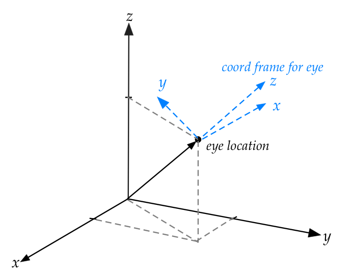
- The eye is located at \((x_E,y_E,z_E) = (15,12,11)\).
- The eye looks straight at the origin.
- Consider the line (the vector) to the eye.
- Then, consider a plane that is between the eye and the origin
and perpendicular (normal) to the line.
- The "2D view" will be on this plane.
- Accordingly, we'll draw the (x,y)-axes on this plane.
- Which means, in 3D, the z-axis will come outwards on
the vector towards the eye.
- This is the desired frame.
- So, the goal is to figure out the transform that will move
the coordinate frame to the desired final frame.
- To do this, we will build a series of transforms
in the forward direction.
- We will compute the inverse of each of these.
- Then, we'll apply the inverses in reverse, multiplying
all of them.
- This will give us the final desired, single transform.
- Apply that transform to a shape will, hopefully, provide
the 2D coordinates that provide the 2D view.
- The "hard work" is to figure out the forward transforms.
- The first one is to translate the origin to the eye.
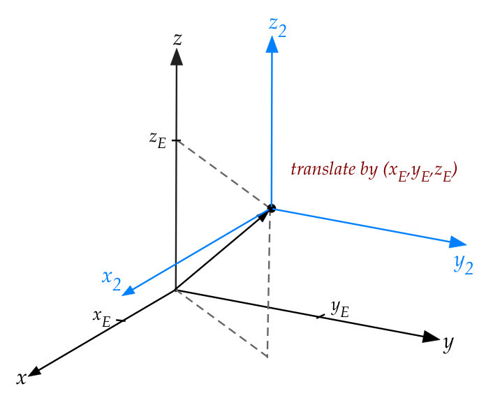
- The (affine) matrix for that is
$$
\mat{1 & 0 & 0 & x_E\\
0 & 1 & 0 & y_E\\
0 & 0 & 1 & z_E\\
0 & 0 & 0 & 1}
$$
- Note: the affine extension for 3D is a \(4 \times 4\) matrix.
- The next one is to slightly twist about the new z-axis:
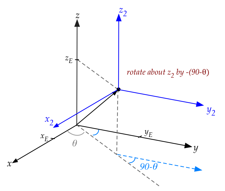
- We're going to align the new y-axis \(y_2\) along the
shadow of the eye vector.
- Which means a rotation of \(90^\circ - \theta\) towards
the x-axis to give:
- By the "right hand rule", we'll use the convention that
this is a rotation of \(-(90^\circ - \theta)\)
- Which results in the affine matrix
$$
\mat{\cos(-(90^\circ - \theta)) & -\sin(-(90^\circ - \theta)) & 0 & 0\\
\sin(-(90^\circ - \theta)) & \cos(-(90^\circ - \theta)) & 0 & 0\\
0 & 0 & 1 & 0\\
0 & 0 & 0 & 1}
$$
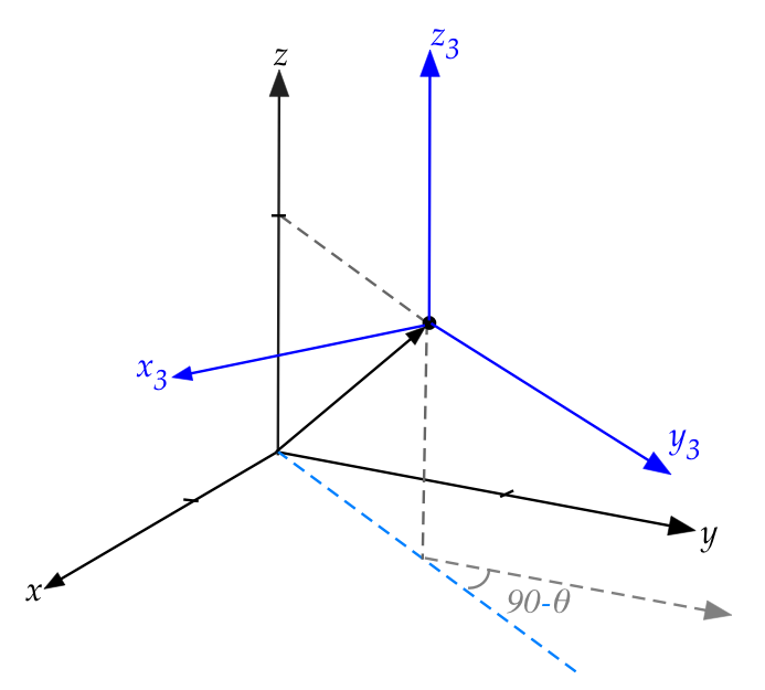
- We'll now do a couple of flips to get the right axis in the
right place.
- First, we'll rotate around the new z-axis by \(180^\circ\):
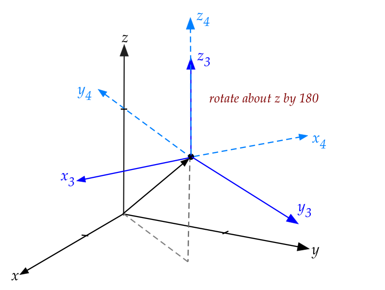
- The matrix for that is:
$$
\mat{\cos(180^\circ) & -\sin(180^\circ) & 0 & 0\\
\sin((180^\circ) & \cos(180^\circ) & 0 & 0\\
0 & 0 & 1 & 0\\
0 & 0 & 0 & 1}
$$
- Next, we'll rotate about the new x-axis (\(x_4\))
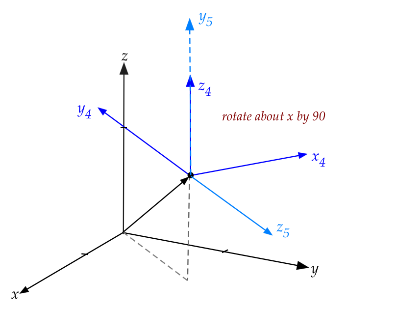
- The matrix for that is:
$$
\mat{\cos(90^\circ) & -\sin(90^\circ) & 0 & 0\\
\sin(90^\circ) & \cos(90^\circ) & 0 & 0\\
0 & 0 & 1 & 0\\
0 & 0 & 0 & 1}
$$
- Lastly, we want to bend the coordinate frame around
the new x-axis (\(x_6\))
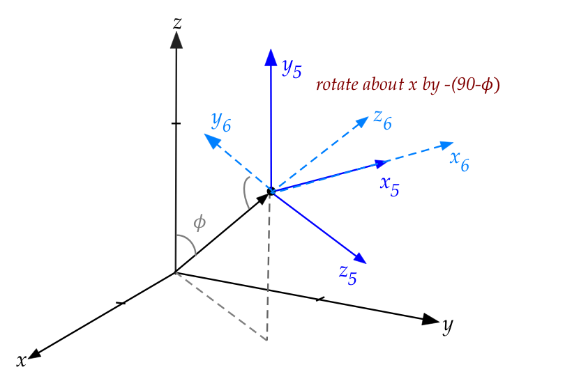
- We want the z-axis to come out towards the eye.
- This means a rotation of \(-(90^\circ - \phi)\) (by the
right-hand convention).
- The matrix:
$$
\mat{\cos(-(90^\circ - \phi)) & -\sin(-(90^\circ - \phi)) & 0 & 0\\
\sin(-(90^\circ - \phi)) & \cos(-(90^\circ - \phi)) & 0 & 0\\
0 & 0 & 1 & 0\\
0 & 0 & 0 & 1}
$$
The next step in the process is to find the inverses:
- The inverse of the translation (let's call this matrix
\({\bf A}_1\))
$$
{\bf A}_1
\eql
\mat{1 & 0 & 0 & -x_E\\
0 & 1 & 0 & -y_E\\
0 & 0 & 1 & -z_E\\
0 & 0 & 0 & 1}
$$
- The inverse of the rotation about the z-axis is
a rotation in the opposite direction:
$$
{\bf A}_2
\eql
\mat{\cos((90^\circ - \theta) & -\sin(90^\circ - \theta) & 0 & 0\\
\sin(90^\circ - \theta) & \cos(90^\circ - \theta) & 0 & 0\\
0 & 0 & 1 & 0\\
0 & 0 & 0 & 1}
$$
- The inverse of the two flips are:
$$
{\bf A}_3
\eql
\mat{\cos(180^\circ) & -\sin(180^\circ) & 0 & 0\\
\sin((180^\circ) & \cos(180^\circ) & 0 & 0\\
0 & 0 & 1 & 0\\
0 & 0 & 0 & 1}
$$
and
$$
{\bf A}_4
\eql
\mat{\cos(-90^\circ) & -\sin(-90^\circ) & 0 & 0\\
\sin(-90^\circ) & \cos(-90^\circ) & 0 & 0\\
0 & 0 & 1 & 0\\
0 & 0 & 0 & 1}
$$
Note: \({\bf A}_3\) is the same because the inverse of
the \(180^\circ\)-flip is another \(180^\circ\)-flip.
- And the last inverse
$$
{\bf A}_5
\eql
\mat{\cos(90^\circ - \phi) & -\sin(90^\circ - \phi) & 0 & 0\\
\sin(90^\circ - \phi) & \cos(90^\circ - \phi) & 0 & 0\\
0 & 0 & 1 & 0\\
0 & 0 & 0 & 1}
$$
- The final transform is then the product of all of these:
\({\bf A} \defn {\bf A}_5{\bf A}_4{\bf A}_3{\bf A}_2{\bf A}_1\)
- Then, the final transform is applied to each original
3D coordinate:
- In our cuboid example, suppose \((x,y,z)\) is a corner.
- We would convert to affine: \((x,y,z,1)\).
- Then multiply by \({\bf A}\) to get the coordinates
\((x',y',z',1)\).
- Use \((x',y')\) as the coordinates in 2D.
- Note: it may sound like computing inverses will be
computationally difficult.
- For a general matrix this is true.
- However, all the coordinate-transformation matrices have
a special property called orthoginality.
- This makes computing the inverse trivial (simply tilt the matrix),
as we'll see.
In-Class Exercise 34:
Examine the code in
CoordChange2D.java
to see all the transforms implemented and multiplied.
Compile and execute to see that we do indeed get
the desired view.
4.10
A closer look at vectors: lengths, angles, orthogonality
The length of a vector:
- Because a vector has a geometric meaning, it's natural to
enquire about its "size".
- The natural size for an arrow-like thing is the length.
- Fortunately, that's easy to calculate by repeated
application of Pythagoras' theorem.
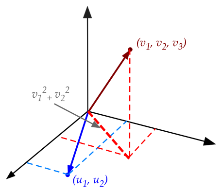
- In two dimensions (blue vector), it's just Pythagoras' theorem:
the squared length of \({\bf u}=(u_1,u_2)\) is
\(u_1^2 + u_2^2\).
- In three dimensions (red vector), we apply Pythagoras'
theorem once to get the length of the projection
onto the first two dimensions.
- And then again, to the right triangle formed by
\((v_1,v_2)\) and \((v_1,v_2,v_3)\).
- Definition: the length of an \(n\) dimensional
vector \({\bf v}\), denoted by \(|{\bf v}|\) is
$$
|{\bf v}| = \sqrt{v_1^2 + v_2^2 + \ldots + v_n^2}
$$
About Pythagoras' theorem:
- Although Pythagoras is credited with the first proof, there is
now evidence of earlier proofs.
- There are over a 100 different proofs.
- Here's one that's historically interesting:
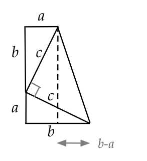
- The right triangle of interest is, of course, the one
with sides \(a, b, c\), which we have copied and
arranged above.
- Can you see why the marked right angle is indeed a right angle?
- The sum of areas of the three triangles are:
\(\frac{ab}{2} + \frac{ab}{2} + \frac{c^2}{2}\).
- The total area can also be calculated as the sum of the
areas of the rectangle and triangle that share the dotted line.
- The rectangle's area: \(a(a+b)\)
- The triangle's: \(\frac{1}{2} (b+a)(b-a)\)
- So, \(\frac{ab}{2} + \frac{ab}{2} + \frac{c^2}{2} =
a(a+b) + \frac{1}{2} (b+a)(b-a)\)
- Which simplifies to \(a^2 + b^2 = c^2\).
The angle between two vectors:
In-Class Exercise 36:
What happens when \({\bf v}={\bf u}\) in
$${\bf v} \cdot {\bf u} \eql |{\bf v}| |{\bf u}| \cos\theta? $$
Norm of a vector:
- The length of a vector \({\bf v}\) can be written as
\(\sqrt{{\bf v} \cdot {\bf v}}\).
- The length is also called the norm.
- There are other types of norms, but the above is
the most common, sometimes called the \(L_2\) norm.
In-Class Exercise 37:
Implement dot product and norm in MatrixTool
and test with NormExample.java.
Orthogonal and orthonormal:
Transpose of a matrix:
- The transpose of an \(m\times n\) matrix \({\bf A}\) is
the \(n\times m\) matrix \({\bf A}^T\) where the i-th row
of \({\bf A}^T\) is the i-th column of \({\bf A}\).
- Another way of saying it: \({\bf A}^T_{ij} = {\bf A}_{ji}\).
- Example:
$$
{\bf A}
\eql
\mat{ 1 & 2 & 3 & 4 & 5\\
6 & 7 & 8 & 9 & 10\\
11 & 12 & 13 & 14 & 15}
\;\;\;\;\;\;\;\;\;\;\;\;\;\;\;\;
{\bf A}^T
\eql
\mat{ 1 & 6 & 11\\
2 & 7 & 12\\
3 & 8 & 13\\
4 & 9 & 14\\
5 & 10 & 15}
$$
In-Class Exercise 39:
If \({\bf A}\) is an orthogonal matrix, what is
\({\bf A^T A}\)? What does this say about the inverse of
\({\bf A}\)? First see what you get with \({\bf A}\) as
the rotation matrix from earlier.
Vector projection:
- Consider two vectors \({\bf u}\) and \({\bf v}\):
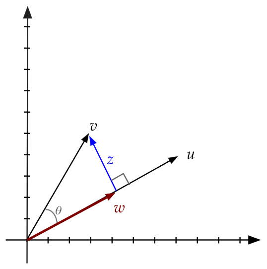
- Let \({\bf w}= \alpha {\bf u}\), a scaled version of \({\bf u}\).
- Let \({\bf z} = {\bf v} - {\bf w}\) so that
\({\bf w} + {\bf z} = {\bf v}\).
- For some \(\alpha\), it's going to be true that \({\bf z}\)
will be perpendicular to \({\bf u}\).
- Clearly at this value of \(\alpha\), we'll have a
right triangle and so, \(|{\bf w}| = |{\bf v}| \cos\theta\)
- Thus,
$$\eqb{
{\bf w}
& \eql &
\alpha {\bf u} \\
& \eql &
\frac{|{\bf w}|}{|{\bf u}|} {\bf u} \\
& \eql &
\frac{|{\bf v}| \cos\theta}{|{\bf u}|} {\bf u} \\
& \eql &
\left(\frac{{\bf u}\cdot {\bf v}}{|{\bf u}| |{\bf u}|} \right) {\bf u} \\
& \eql &
\left(\frac{{\bf u}\cdot {\bf v}}{{\bf u}\cdot {\bf u}} \right) {\bf u} \\
}$$
where we substituted \(\cos\theta = \frac{{\bf u}\cdot {\bf v}}{|{\bf u}| |{\bf v}|}\)
- In other words:
$$
\alpha \eql
\left(\frac{{\bf u}\cdot {\bf v}}{{\bf u}\cdot {\bf u}} \right)
$$
- Thus, the term \(\left(\frac{{\bf u}\cdot {\bf v}}{{\bf
u}\cdot {\bf u}} \right)\) gives us a number to multiply
into \({\bf u}\) that will stretch \({\bf u}\) so that the
stretched vector \({\bf w}\) is the projection of \({\bf v}\).
- The vector \({\bf w}\) is called the projection
of \({\bf v}\) onto \({\bf u}\)
- We'll write \(\mbox{proj}_{\bf u}({\bf v}) = {\bf w}\)
so that
$$
\mbox{proj}_{\bf u}({\bf v})
\eql
\left(\frac{{\bf u}\cdot {\bf v}}{{\bf u} \cdot {\bf u}} \right) {\bf u} \\
$$
- Note:
- What's inside the parens above evaluates to a single number:
\(\rhd\)
This becomes a scalar that multiplies into \({\bf u}\)
- \(\mbox{proj}_{\bf u}({\bf v})\) is in the same direction as
\({\bf u}\)
- \({\bf z} = {\bf v} - \mbox{proj}_{\bf u}({\bf v})\) is always
perpendicular to \({\bf u}\).
- Also, if \({\bf u}\) is a unit vector, then
$$
\mbox{proj}_{\bf u}({\bf v})
\eql
\left( {\bf u}\cdot {\bf v} \right) {\bf u} \\
$$
since \({\bf u}\cdot {\bf u} = 1\) for any unit-length vector.
In-Class Exercise 40:
Implement projection in MatrixTool and test with
ProjectionExample.java.
Confirm that you get the same vectors as in the diagram above.
4.11
Review: what does inverse mean?
Let's step back for a moment and get more comfortable with the
notation \({\bf A}^{-1}\). Does it mean raising a matrix to the power -1?
Let's see:
- First, let's examine how inverse works for numbers.
- If \(x,y,z\) are three numbers such that
$$
x y \eql z
$$
- Then, to solve for \(y\) multiply both sides by \(\frac{1}{x}\)
$$
\frac{1}{x} x y \eql \frac{1}{x} z
$$
Which means
$$
y \eql \frac{1}{x} z
$$
- We use the notation \(x^{-1}\) to mean the multiplicative
inverse \(x^{-1} = \frac{1}{x}\) where \(x^{-1}\) satisfies
$$
x^{-1} x \eql 1
$$
Here, 1 is the multiplicative identity.
- Thus, we can write
$$
y \eql x^{-1} z
$$
- For numbers, it so happens that \(x^{-1}\) is in fact
"raising \(x\) to the power -1."
- But for matrices, it's best to read the superscript \(-1\) as just
a symbol to denote this inverse, rather than "raising to power
-1"
- Analogous to what we did with numbers,
consider a matrix multiplying into a vector:
$$
{\bf A}{\bf u} \eql {\bf v}
$$
- If there was a matrix inverse (another matrix) \({\bf A}^{-1}\)
such that multiplying on both sides
$$
{\bf A}^{-1} {\bf A} {\bf u} \eql {\bf A}^{-1}{\bf v}
$$
simplifies to
$$
{\bf u} \eql {\bf A}^{-1}{\bf v}
$$
then we'd have a convenient way to solve for \({\bf u}\), if we
know \({\bf v}\).
How does one compute the inverse of a matrix?
- We've seen two ways so far:
- Use geometric intuition: the inverse of the matrix
that rotates by \(60^\circ\) must be the matrix that
rotates by \(-60^\circ\).
- The inverse of an orthogonal matrix is its transpose.
- Of course, we want to be able to compute the inverse
for any matrix.
- What we'll learn (this will take some work) later is that:
- Not all matrices have inverses (and we can detect that).
- When a matrix has an inverse, we'll be able to compute it.
- If a matrix does not have an inverse, we can compute
something that's approximately an inverse.
4.12
Understanding change-of-basis via orthogonality and projections
Many presentations of change-of-basis (especially in graphics)
use the properties of orthogonal vectors, which can hide the
intuition.
So, let's untangle that type of presentation given what we've just learned.
We'll do this in many steps.
Step 1: recall key points from orthogonality and projections:
- Two vectors are orthogonal if their angle is \(90^\circ\).
- Because
$$
{\bf v} \cdot {\bf u}
\eql
|{\bf v}| |{\bf u}|
\cos(\theta)
$$
that's the same thing as saying \({\bf v}\) and \({\bf u}\)
are orthogonal if \({\bf v} \cdot {\bf u} = 0\),
(because \(\cos(90^\circ) = 0\)).
- \({\bf v}\) and \({\bf u}\) are orthonormal
if they are orthogonal AND their lengths are 1 (unit length).
- If a matrix \({\bf A}\) has columns that are orthonormal,
then
$$
{\bf A}^{-1} \eql {\bf A}^T
$$
(Exercise 39 above)
- The projection of any vector \({\bf v}\) on a unit vector
\({\bf u}\) is the vector
$$
\mbox{proj}_{\bf u}({\bf v})
\eql
\left( {\bf u}\cdot {\bf v} \right) {\bf u} \\
$$
- Observe: the dot product \({\bf u}\cdot {\bf v}\)
gives us the "stretch factor" (a number).
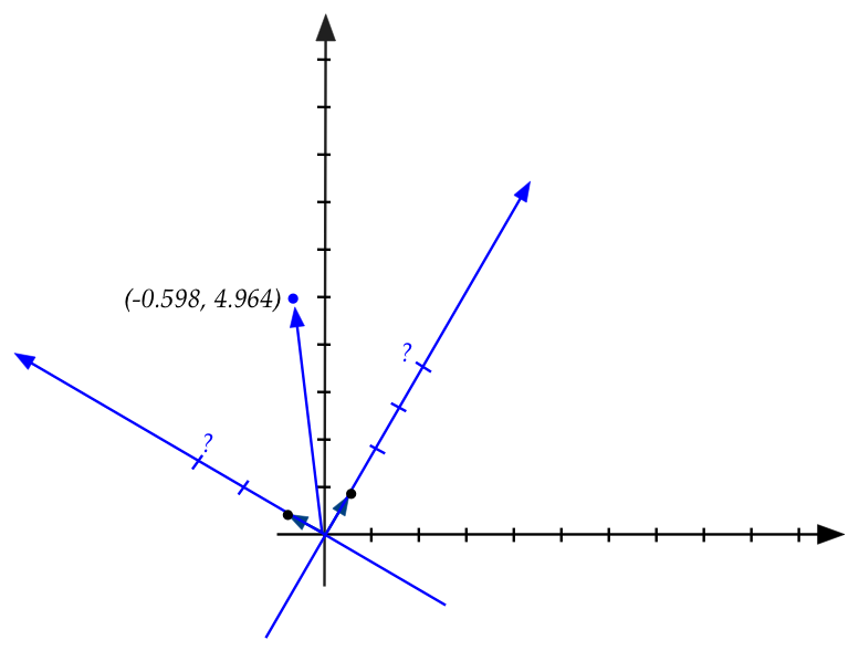
Step 2: what's the goal when we change coordinates?
- We are given a vector \({\bf v}\) in standard coordinates, e.g.,
$$
{\bf v} \eql \vectwo{-0.598}{4.964}
$$
- We want the coordinates of this point when the axes are
rotated by, say, \(60^\circ\):
Step 3: recall our direct approach from earlier:
- Figure out what the unit vectors will be in the new system:
- This requires reasoning in geometry as in:
- In this case, we get
$$
\mat{\cos(\theta) & -\sin(\theta)\\
\sin(\theta) & \cos(\theta)}
\approx
\mat{0.5 & -0.866\\ 0.866 & 0.5}
$$
- Then, we ask: what are the coordinates in the new system
\({\bf v}^\prime = (v_1^\prime, v_2^\prime)\) such that
$$
\mat{0.5 & -0.866\\ 0.866 & 0.5}
\vectwo{v_1^\prime}{v_2^\prime}
\eql
\vectwo{-0.598}{4.964}
$$
- Suppose we use the symbol \({\bf A}\) for the matrix
$$
{\bf A} \eql
\mat{0.5 & -0.866\\ 0.866 & 0.5}
$$
and
$$
{\bf v} \eql
\vectwo{-0.598}{4.964}
$$
we can state this compactly as
$$
{\bf A} {\bf v}^\prime \eql {\bf v}
$$
- Left-multiplying each side by \({\bf A}^{-1}\):
$$
{\bf A}^{-1} {\bf A} {\bf v}^\prime \eql {\bf A}^{-1} {\bf v}
$$
which means
$$
{\bf I} {\bf v}^\prime \eql {\bf A}^{-1} {\bf v}
$$
which further means
$$
{\bf v}^\prime \eql {\bf A}^{-1} {\bf v}
$$
- So, if we could somehow compute the "undo" (inverse)
of the \({\bf A}\) matrix, we'd be done.
- So far we've not studied how to compute an inverse,
merely that such things exist.
- For a clockwise rotation by \(60^\circ\) we saw that
the inverse is the matrix for counter-clockwise rotation by
\(60^\circ\), which turned out to be:
$$
{\bf A}^{-1} \eql
\mat{0.5 & 0.866\\ -0.866 & 0.5}
$$
- Then, we'd get
$$
\vectwo{4}{3}
\eql
\mat{0.5 & 0.866\\ -0.866 & 0.5}
\vectwo{-0.598}{4.964}
$$
These are the new coordinates:
- Notice: the new unit vectors happen to be the
rows of \({\bf A}^{-1}\). A coincidence?
Step 4: let's apply our new understanding of orthogonality
- First observe that the columns of \({\bf A}\) are
the unit vectors in the new coordinate system.
- Key observation: the unit vectors are orthonormal.
- This means the columns of \({\bf A}\) are orthogonal.
- Which means
$$
{\bf A}^{-1} \eql {\bf A}^T
$$
- Thus, to build the inverse of \({\bf A}\), simply transpose it.
- Therefore, the rows of \({\bf A}^T\) are the columns of \({\bf A}\).
- So, a (less intuitive) way of doing a change-of-axes is to
say:
- Build a matrix with the unit vectors in the new system
as rows.
- Multiply into old coordinates to get new coordinates.
Step 5: apply our new understanding of projections
- Suppose we call the original unit vectors
$$
{\bf e}_1 \eql \vectwo{1}{0}
\;\;\;\;\;\;
{\bf e}_2 \eql \vectwo{0}{1}
$$
and the new unit vectors
$$
{\bf e}_1^\prime \eql \vectwo{0.5}{0.866}
\;\;\;\;\;\;
{\bf e}_2 \prime \eql \vectwo{-0.866}{0.5}
$$
- Then, the rows of \({\bf A}^T\) are:
$$
{\bf A}^{-1} \eql {\bf A}^T \eql
\mat{
\ldots & {\bf e}_1^\prime & \ldots \\
\ldots & {\bf e}_2^\prime & \ldots
}
$$
- So, when we multiply to get the new coordinates, we
are multiplying
$$
{\bf v}^\prime \eql
{\bf A}^T {\bf v}\eql
\mat{
\ldots & {\bf e}_1^\prime & \ldots \\
\ldots & {\bf e}_2^\prime & \ldots
}
{\bf v}
$$
- Each row of \({\bf A}^T\) gets multiplied into
the vector \({\bf v}\):
$$
{\bf v}^\prime \eql
\vectwo{{\bf e}_1^\prime \cdot {\bf v}}{{\bf e}_2^\prime \cdot {\bf v}}
$$
- Recall: for a unit vector, this is just the "projection stretch"
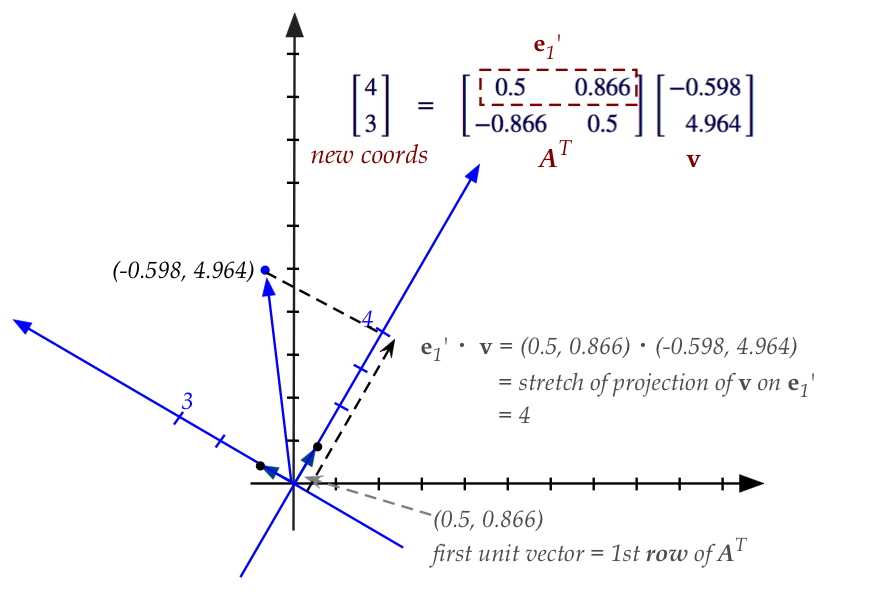
- We are able to easily see this stretch geometrically in the
picture above.
That was a lot to understand. Let's summarize:
- Our from-the-ground approach simply used vector-stretches to
get coordinates in the new system.
- The vectors themselves are the new unit vectors as columns
of the matrix \({\bf A}\).
- If we know how to compute inverses, we just apply the
inverse to old coordinates to get new ones.
- But now that we know that \({\bf A}\) is orthogonal,
the inverse is simply \({\bf A}^T\).
- Further interpretation shows that each row of \({\bf A}\),
which is one of the new unit vectors, multiplies into
the old coordinates to give the "projection stretch" in the
unit vector's direction.
- This "stretch" is in fact the coordinate in that direction.
- Whew!
4.13
Complex vectors
Before proceeding, you are strongly advised to first review complex numbers
from Module 2.
So far, the vectors we've seen have had real numbers as elements
\(\rhd\)
We could call them real vectors
A vector with complex numbers as elements is a complex vector:
- Thus, if \(2 + 3i\) and \(5 - 4i\) are two complex numbers,
the vector \((2+3i, 5-4i)\) is a 2D complex vector.
- In general, a complex vector of \(n\) dimensions will have
\(n\) complex numbers as elements:
$$
(a_1+ib_1, a_2+ib_2, \ldots, a_n+ib_n)
$$
- In column form:
$$
\vecdots{a_1+ib_1}{a_2+ib_2}{a_n+ib_n}
$$
- What remains is to see how the operations on real vectors
can be extended to complex vectors.
- Addition is a straightforward extension:
- Let \({\bf u} = (u_1,\ldots,u_n)\) and
\({\bf v} = (v_1,\ldots,v_n)\) be two complex vectors.
- Here, each \(u_i\) and \(v_j\) are complex numbers,
with real and imaginary parts.
- Then,
$$
{\bf u} + {\bf v} \eql
(u_1 + v_1, u_2 + v_2, \ldots, u_n + v_n)
$$
- Each \(u_i + v_i\) is complex addition.
In-Class Exercise 41:
What is the sum of \((1+2i, i, -3+4i, 5)\)
and \((-2+i,2,4,1+i)\)?
(Note: each has 4 components.)
- Scalar multiplication is a bit different in that
the scalar can now be a complex number:
$$\eqb{
\alpha {\bf u}
& \eql &
\alpha (u_1,u_2,\ldots,u_n) \\
& \eql &
(\alpha u_1, \alpha u_2, \ldots, \alpha u_n)
}$$
- Here, both \(\alpha\) and each \(u_i\) are complex numbers.
- Thus, the rules of complex multiplication are needed
for calculating each \(\alpha u_i\).
In-Class Exercise 42:
What is the scalar product of \(\alpha = (1-2i)\)
and \({\bf u}= (1+2i, i, -3+4i, 5)\)?
- So far, operations for complex vectors look like their
real counterparts.
- The dot product, however, is an exception.
- For complex vectors \({\bf u}\) and \({\bf v}\), the
dot product is defined as
$$
{\bf u} \cdot {\bf v} \eql
u_1 \overline{v_1} + u_2 \overline{v_2} + \ldots +
u_n \overline{v_n}
$$
- Recall: for a complex number \(z=a+bi\),
\(\overline{z} = \mbox{conjugate}(z) = a-bi\).
- The obvious question is, of course, why?
\(\rhd\)
It has to do with the relationship between magnitude and dot-product.
- For a real vector \({\bf u} = (u_1,u_2,\ldots,u_n)\)
- \(\mbox{magnitude}({\bf u}) = |{\bf u}|
= \sqrt{|u_1|^2 + |u_2|^2 + \ldots + |u_n|^2}\)
- In other words, \(|{\bf u}| = \sqrt{\mbox{sum of squared
magnitudes of elements of }{\bf u}}\)
- For a real number \(u_i\), the squared-magnitude is simply
\(|u_i|^2 = u_i^2 = u_i \times u_i\)
- Not so for a complex number.
- The squared magnitude of the complex number
\(a+bi\) is \(a^2 + b^2\), which is the distance from the origin:
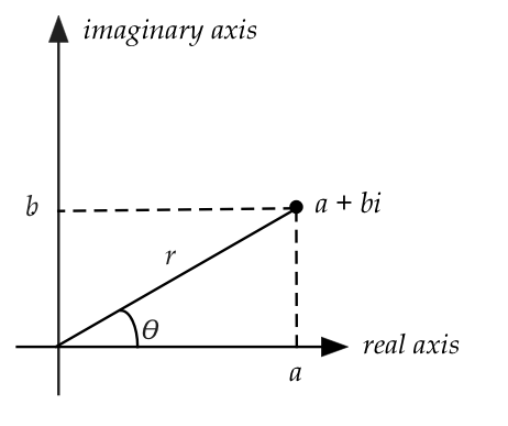
Note: \(a^2 + b^2 \neq (a+bi)(a+bi)\)
But \(a^2 + b^2 = (a+bi)(a-bi)\)
In-Class Exercise 43:
Work out the two products \((a+bi)(a+bi)\)
and \((a+bi)(a-bi)\).
- What does this have to do with the dot-product?
- For real vectors,
$$\eqb{
{\bf u} \cdot {\bf u}
& \eql &
(u_1,u_2,\ldots,u_n) \cdot (u_1,u_2,\ldots,u_n) \\
& \eql &
u_1^2 + u_2^2 + \ldots + u_n^2 \\
& \eql &
|u_1|^2 + |u_2|^2 + \ldots + |u_n|^2\\
& \eql &
|{\bf u}|^2
}$$
- To make this work for complex numbers:
$$\eqb{
{\bf u} \cdot {\bf u}
& \eql &
(u_1,u_2,\ldots,u_n) \cdot (\overline{u_1},\overline{u_2},\ldots,\overline{u_n}) \\
& \eql &
u_1 \overline{u_1} + u_2 \overline{u_2} +
\ldots + u_n\overline{u_n} \\
& \eql &
|u_1|^2 + |u_2|^2 + \ldots + |u_n|^2 \\
& \eql &
|{\bf u}|^2
}$$
In-Class Exercise 44:
For the complex vector \({\bf z}=(z_1,z_2,z_3) = (1+2i, i, 5)\), compute
both \({\bf z} \cdot {\bf z}\) and
\(z_1^2 + z_2^2 + z_3^2\).
Why complex vectors (and matrices) are important:
- Complex numbers are at the foundation of Fourier series
and Fourier transforms.
- The Discrete Fourier Transform (DFT), in particular:
- Is formulated as a matrix-vector multiplication.
- Uses complex numbers for both practical and theoretical reasons.
- Extracts useful information even from the imaginary
parts of the complex numbers.
- Much of the theoretical development of advanced linear
algebra uses complex numbers.
- Numerical methods for linear algebra are based on the theory
developed with complex vectors and matrices.
- All of quantum computing (and quantum mechanics) is founded
on the linear algebra of complex vectors (vectors with complex numbers).
Dot product convention:
- Most books use the dot-product definition above:
$$
{\bf u} \cdot {\bf v} \eql
u_1 \overline{v_1} + u_2 \overline{v_2} + \ldots +
u_n \overline{v_n}
$$
- However, in some contexts, the left vector is conjugated:
\({\bf u} \cdot {\bf v} \eql
\overline{u_1} v_1 + \overline{u_2} v_2 + \ldots +
\overline{u_n} v_n\)
- Consider the complex numbers \(u_1=(2+3i)\) and
\(v_1=(3+4i)\). Then
$$\eqb{
u_1 \overline{v_1} & \eql & (2+3i) \overline{(3+4i)}
& \eql & (2+3i) (3-4i)
& \eql & (18 + i) \\
\overline{u_1} v_1 & \eql & \overline{(2+3i)} (3+4i)
& \eql & (2-3i) (3+4i)
& \eql & (18 - i) \\
}$$
- So, the definitions will result in different dot-products
but \({\bf u}\cdot{\bf u} = |{\bf u}|^2\) still holds,
and the real part is the same.
- The convention in physics and quantum computing is to left-conjugate.
4.14
Exploring the action of some matrices on vectors
We will end this module by exploring how some matrices transform
vectors.
We'll start with orthogonal matrices:
- First, we will generate a random orthogonal matrix and
apply it to a few vectors.
- To create a random orthogonal matrix, we'll use the unit circle:
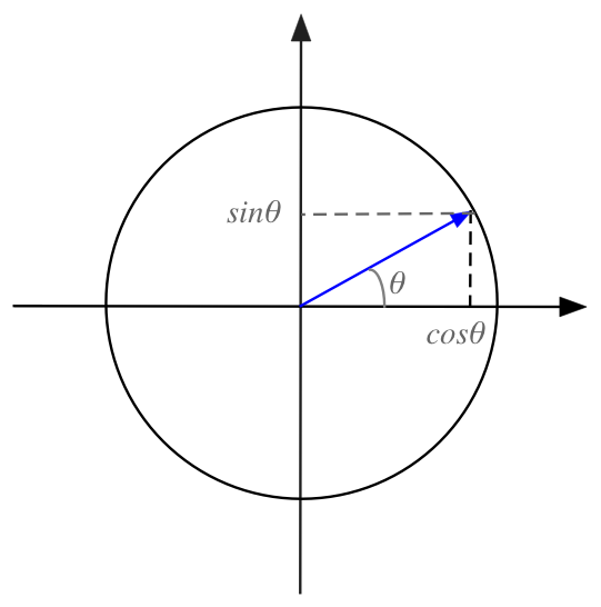
- Generate a random angle \(\theta\) and use
\((\cos\theta, \sin\theta)\) as the first column.
- Use \((\cos(\theta + 90^\circ), \sin(\theta + 90^\circ))\)
as the second column.
\(\rhd\)
This way, the second column is perpendicular (orthogonal) to
the first.
In-Class Exercise 45:
Examine the code in
OrthoExplore.java
to confirm the generation method. You will also
need UniformRandom.java
(for this, and other exercises).
Run a few times to see the results.
Confirm that the matrix rotates the vectors but does not change
their length.
- Next, we will generate a random orthogonal matrix and apply it
systematically to a number of vectors.
- To choose which vectors to apply a matrix to, we will
merely choose equally spaced vectors on the unit circle:
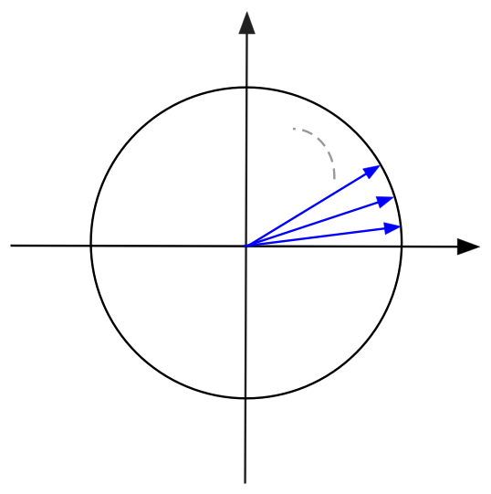
- Then, to see what the matrix does, we'll identify the
change of angle (ignoring the length):
        A = random orthogonal matrix
        for θ=0 to 2π
           u = (cosθ, sinθ)     // Thus, θ is u's angle from the x-axis
           z =  A u
           α = angle of z       // From the x-axis
	   Add (θ, α) to data set
        endfor
        Plot data set
In-Class Exercise 46:
Examine the code in
OrthoExplore2.java
to confirm the above approach.
You will also need Function.java
and SimplePlotPanel.java.
Run a few times to see the results.
Explain the graph of \(\alpha\) vs. \(\theta\).
Non-orthogonal matrices:
Let's dig a little deeper into that point of intersection above.
In-Class Exercise 48:
Examine the code in
MatrixExplore2.java
to see that it's a simple example of a matrix that transforms
the vector \({\bf u}=(1,2)\) into another vector.
Compile and execute to draw the two vectors.
Then try \({\bf u}=(1,0)\)
We will now start with a vector and repeatedly apply
the matrix in sequence:
    u = any vector
    draw (u)
    for i=0 ...
       u = A u
       draw (u)
    endfor
In-Class Exercise 49:
Examine the code in
MatrixExplore3.java
to see that the same matrix as in the previous
exercise iteratively multiplies as above.
What do you observe?
Try a larger number of iterations,
and different starting vectors.
Finally, let's see what happens when a random matrix
is iteratively applied to a starting vector.
In-Class Exercise 50:
The program
MatrixExplore4.java
produces a random matrix each time it's executed. This
matrix is applied iteratively to a starting vector.
How often do you see fixed points emerging?
Some questions that arise at this point:
- Is it true that all orthogonal matrices only affect the angle
in transforming a vector?
- What kinds of matrices applied to a vector merely stretch
(but do not rotate) the vector?
- Does iterative application of a matrix always lead to a
fixed point?
- What can we say about any random matrix in general?
A preview of things to come:
- Yes, orthogonal matrices only affect angle (and are useful in
applications)
- A fixed point like the one above is called an eigenvector.
- Repeated application of the matrix often leads to an
eigenvector.
\(\rhd\)
This will turn out to be the secret behind the page rank algorithm.
- The most remarkable result of all: every matrix is a
combination of an generalized rotation, followed by a stretch, followed
by another generalized rotation.
\(\rhd\)
This is the famous singular value decomposition (SVD)
4.15
Highlights and study tips
Highlights:
- A matrix applied (by left multiplication) to a vector
produces another vector
\(\rhd\)
We can call this a transformation
- Note: Matrix multiplication can also be interpreted as a linear
combination of the matrix's columns.
\(\rhd\)
This is useful in deriving transformations.
- A sequence of matrix multiplications causes transformations
to occur in sequence.
\(\rhd\)
The product of the matrices produces the combined transformation.
- Matrix multiplication is associative and distributes over
addition, but is not commutative.
- The span of a collection of vectors is the set of all
vectors you can get with linear combinations of the collection.
- Given a set of vectors, a basis is a minimal set whose
span is the set.
- Transforms are engineered by expressing transformed unit
basis vectors, and placing those in a matrix as columns.
- The affine extension allows us to express translation as
a matrix transformation.
- The matrix \({\bf A}^{-1}\) is the inverse of
of matrix \({\bf A}\) if \({\bf A}^{-1} {\bf A} = {\bf I}\)
where \({\bf I}\) is the identity matrix.
- Important vector definitions to review: norm (length), angle
between two vectors, dot product, orthogonal, orthonormal,
transpose, projection.
- Important matrix definitions: orthogonal, transpose, affine
extension, identity, inverse.
- Remember: another view of matrix-matrix multiplication is that
the matrix on the left multiplies each column of the matrix
on the right.
How to review:
- There were a lot of new ideas in this module.
- It's best to sort out the definitions carefully. They
will be needed in later modules.
- You can come back to the geometric transformations whenever needed.