Module objectives
By the end of this module, you should be able to
- Explain what vectors and matrices are and why
they are defined in the way they are.
- Perform simple computations with vectors and matrices.
- Solve by hand some matrix-vector equations.
- Describe the different ways of interpreting the matrix-vector
equation.
3.0
A collection of numbers as a mathematical object
At a very basic level, every application we saw computes with
numbers.
\(\rhd\)
An organized series of operations on numbers.
A closer look reveals that some numbers naturally fall into groups:
- For example, consider application #1: linear equations
- The coefficients of a single equation are clearly related.
- All the right-hand-side numbers could be a group.
- Application #3: Bezier curves
\(\rhd\)
The coordinates of the control points.
- Application #6: Image search
\(\rhd\)
All the numbers (intensity values) in an image.
In-Class Exercise 1:
Pick three other applications and propose natural groupings
of numbers for those applications.
What do we know from math thus far about groups of numbers?
- Set theory is one possibility.
- For example, \(\{1,4,9,16\}\) is a group of related numbers.
- What can one do with sets?
- The usual binary operators: \(\cup, \cap\)
- Can one "add" two sets?
- One practical problem with set theory:
- Real applications actually operate (add, multiply, etc) on
actual numbers.
- The set theory operators do not result in operations on numbers.
- Thus, there is no \(+\) operator for sets that results in
number addition,
\(\rhd\)
e.g., something like \(\{1,2,3\} + \{2,3,4\} = \{3,5,7\}\)
- We could define such operators, but would run into
issues with order:
- Example: we know \(\{1,2,3\} = \{3,2,1\}\)
\(\rhd\)
Then is \(\{3,2,1\} + \{2,3,4\} = \{3,5,7\}\)?
What we would like:
- A mathematical object to hold a collection of numbers.
- Definitions of operators like \(+,\times\)
on collections such that:
- There is no ambiguity.
- An operator applied to a collection has a natural way
of devolving to the numbers in the collection.
The answer: a tuple
- A tuple is an ordered collection of numbers.
- Examples:
- \((1,2,3)\) is a tuple.
- The tuple \((1,2,3)\) is different from \((2,1,3)\) and from
\((1,2,3,3)\).
- We aren't restricted to integers: \((1.414, 2.718, 3.141)\)
is a tuple.
- An \(n\)-tuple is a tuple with \(n\) elements.
- What can we do with tuples? Let's define addition and
multiplication as:
- Addition of two tuples:
$$
(u_1,u_2,\ldots,u_n) + (v_1,v_2,\ldots,v_n) =
(u_1+v_1, \; u_2+v_2, \; \ldots, \;u_n+v_n)
$$
- Example:
$$
(1,2,3) + (4,5,6) = (1+4, 2+5, 3+6) = (5,7,9)
$$
- Multiplication:
$$
(u_1,u_2,\ldots,u_n) \cdot (v_1,v_2,\ldots,v_n) \;\; = \;\;
u_1 v_1 + u_2 v_2 + \ldots + u_n v_n
\;\; = \;\;
\sum_{i=1}^n u_i v_i
$$
\(\rhd\)
The result is a single number.
- Example:
$$
(1,2,3) \cdot (4,5,6) = 1\times 4 + 2\times 5 + 3\times6
= 4 + 10 + 18 = 32
$$
- Note:
- Multiplication is unexpectedly different from addition. It's
not clear (yet) why we should do this.
- Both tuples above in addition or multiplication have to have
the same number of elements.
- Subtraction follows from defining addition.
- We'll put division on hold for now, until we get
to inverses.
- We'll also be interested in operators that combine a single
number and the collection.
- For real number \(\alpha\) and tuple \((v_1,v_2,\ldots,v_n)\),
define scalar multiplication as
$$
\alpha (v_1,v_2,\ldots,v_n) \;\; = \;\;
(\alpha v_1, \alpha v_2,\ldots, \alpha v_n)
$$
- One could conceive of an equivalent scalar addition
but it turns out not to be useful.
Continuing this exploration, let's ask: is there a useful geometric
interpretation for tuples?
- We've certainly seen a 2-tuple like \((1,2)\) before.
\(\rhd\)
A point in the 2D plane.
- Similarly, one could say that a 3-tuple is a 3D point, and
so on.
Two problems with tuples-as-points:
- First, there's the meaning of point addition:
in what way are we seeing two things being added?
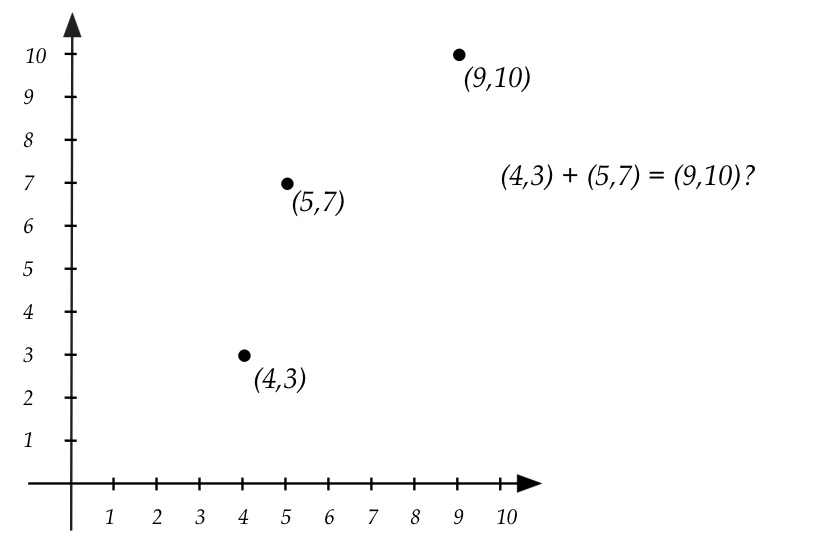
- Second, we get inconsistent results if the frame of
reference (coordinate system) changes:
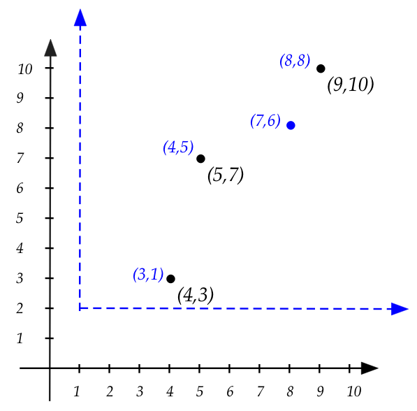
- Above, to get "blue" coordinates from black coordinates,
we shift by \((1,2)\)
\(\rhd\)
e.g., \(\color{blue}{(3,1)} = \color{black}{(4,3) - (2,1)}\)
- But the added points in black gives us: \((9,10)\),
which is \(\color{blue}{(8,8)}\) when shifted.
\(\rhd\)
This is not equal to the direct addition, which gives
\(\color{blue}{(7,6)}\)
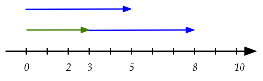
To resolve this, let's go back to 1D:
- Let's look at adding \(5 + 3\) on the number line:
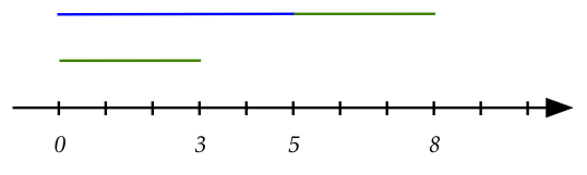
- Suppose we think of \(3\) and \(5\) as lengths from \(0\).
- Then, we are adding the length \(3\) at the end of
the length going from \(0\) to \(5\).
- Thus, even though \(3\) and \(5\) are "points" on the
number line, we can also interpret them as lengths.
- Put differently, the "length 3" is moved to the point "5".
- Once so moved, the resulting length ends at the point "8".
\(\rhd\)
(Which represents length 8).
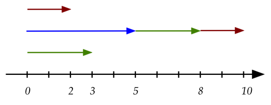
- Written as tuples in 2D, we could say that
\((5,0) + (3,0) = (8,0)\).
- The understanding here is that we take the "length 3"
and move that to the end of the point \((5,0)\)
to get the point \((8,0)\)
- There is one more detail to worry about:
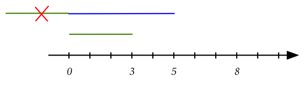
- We cannot move the "length 3" to the other end of the \(5,0\)
segment.
- Doing so, would give us the point \((-3,0)\) and
\((-3,0) \neq (5,0)+(3,0)\)
- Thus, there is an inherent preference or labeling of
which "end" of a segment.
- The convention we'll use to label the desired end is to
use an arrowhead:
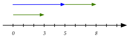
- Notice that the segment \((3,0)\) also has an arrowhead.
- This makes sense for two reasons:
- Notice that it works for negative numbers as well:
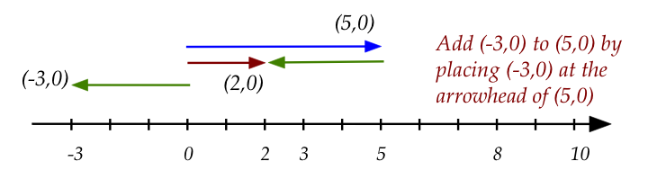
- We maintain the direction of \((-3,0)\) when
placing its tail at the head of \((5,0)\).
- The result is the red arrow, \((2,0)\).
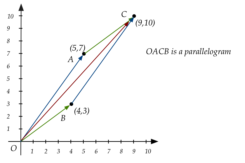
We'll now make this work for 2D:
- Let the tuple \((x,y)\) be associated with the arrow going from
\((0,0)\) to the point \((x,y)\).
- For example:
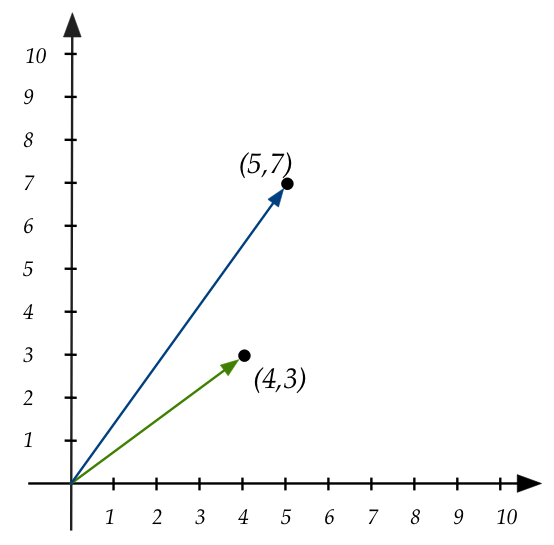
- To add \((4,3)\) and \((5,7)\), slide the arrow corresponding
to \((4,3)\) so that it's tail touches the arrowhead of \((5,7)\):
\(\rhd\)
The result is the arrow to \((9,10)\):
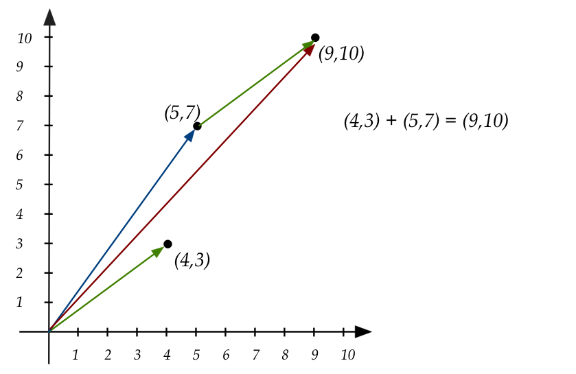
- Note: we don't change the orientation (direction) of the arrow when
we move it.
- There is an important point to make using the above example:
- The arrow drawn between \((5,7)\) and \((9,10)\) doesn't
really exist as a tuple.
- It is moved there only to illustrate addition.
- The technically correct illustration is:
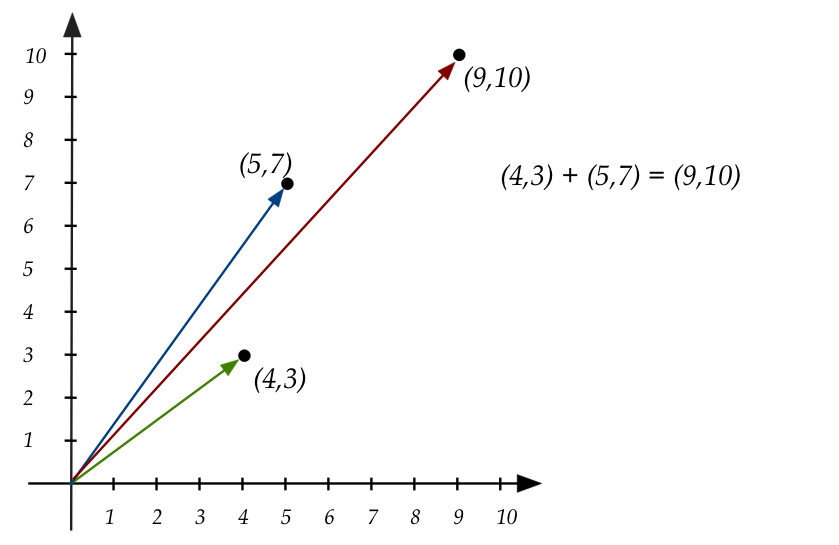
- The only correct arrow is one that has its tail at
\((0,0)\).
- However, we will draw "moved" arrows because they make it
easier to visualize operations and results.
- Arrows of the type above are called vectors.
- Because tuples now have vectors as a geometric interpretation,
we don't need two terms for the same thing.
\(\rhd\)
We will use the term vector henceforth.
In-Class Exercise 2:
Explain the following:
- Go back to the example with two coordinate systems, and verify
by hand that addition produces the same result, relative
to the new origin.
- What would be the case if a second set of coordinate axes
had the same origin but was rotated slightly (say, by 60 degrees)?
- By the rules above, we aren't allowed to change the orientation
of an arrow when it's moved for addition. Why is that? What would
go wrong with the theory if we allowed the direction to change?
3.1
Vectors
Vector notation:
- There are three types of notation for vectors.
- Consider the vector \((v_1,v_2,\ldots,v_n)\).
- This is often written in short form as one of these:
- \({\bf v} = (v_1,v_2,\ldots,v_n)\)
(boldface)
- \(\vec{v} = (v_1,v_2,\ldots,v_n)\)
(arrow)
- \(\stackrel{\rightharpoonup}{v} = (v_1,v_2,\ldots,v_n)\)
(harpoon)
- We will generally prefer boldface, and occasionally the arrow.
- When you write
homeworks by hand it's hard to boldface: use the arrow instead.
The parallelogram law:
Next, let's look at scalar multiplication
- Recall:
$$\eqb{
\alpha {\bf v}
& \;\; =\;\; &
\alpha (v_1, v_2, \ldots, v_n) \\
& \;\; =\;\; &
(\alpha v_1, \alpha v_2, \ldots, \alpha v_n) \\
}$$
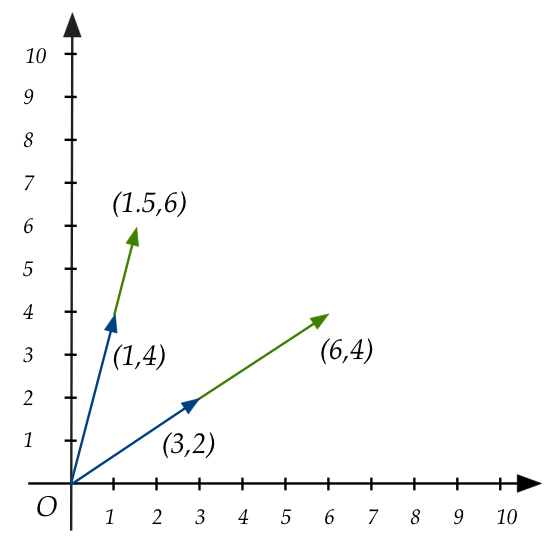
- Example: \( 2 (3,2) = (6,4)\)
- Example: \( 1.5 (1,4) = (1.5,6)\)
- Let's draw these:
- Another example: \(-0.5 (3,2)\)
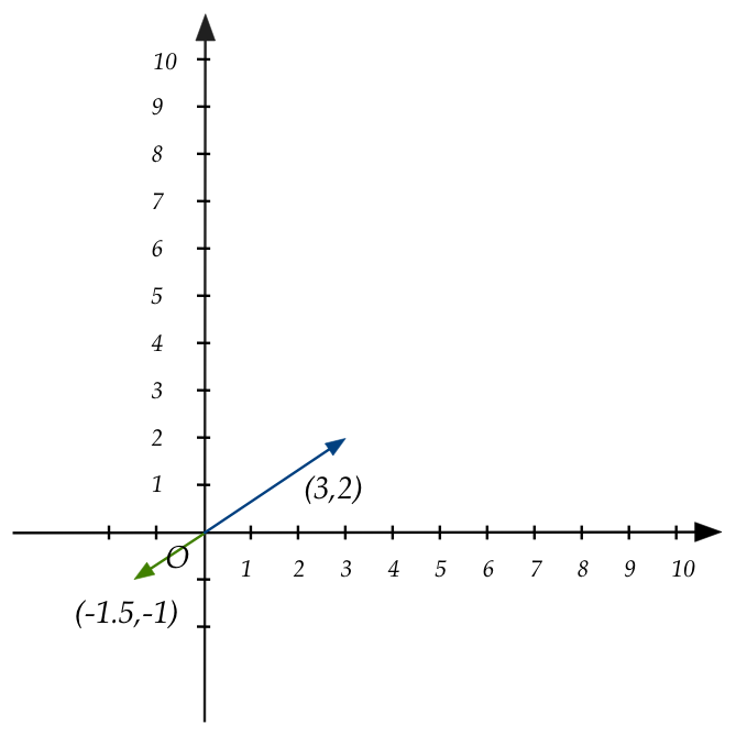
- Thus, scalar multiplication "stretches" or "shrinks",
and can also flip direction if the scalar is negative.
- We will generically use "stretch" to mean any of the above.
- A negative stretch flips direction.
- A fractional stretch actually shrinks.
In-Class Exercise 3:
Why is it true that the orientation (angle), except for flips, is unchanged by
scalar multiplication?
A special vector: the zero vector
- We will use the notation \({\bf 0}\) to denote
the vector containing all zeroes:
\({\bf 0} = (0,0,\ldots,0)\).
- Obviously, for any vector \({\bf u}\),
we have \({\bf u} + {\bf 0} = {\bf u}\)
\(\rhd\)
\({\bf 0}\) is the additive identity for vector addition.
- Similar to numbers, \({\bf u} \cdot {\bf 0} = 0\)
\(\rhd\)
Here, the right hand side is the number \(0\),
not the vector \({\bf 0}\).
3.2
Linear combinations
Let's now consider an all-important idea: a linear combination
- A linear combination of vectors is a vector.
- Each vector in the combination is first stretched,
and then all the stretched vectors are added.
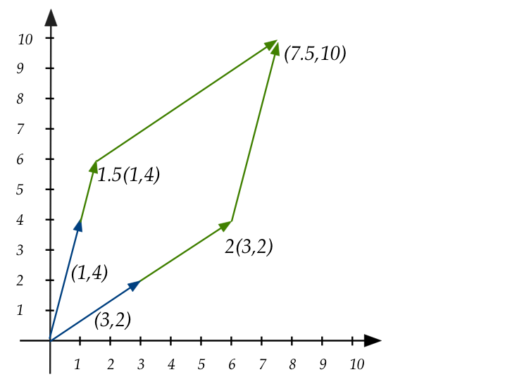
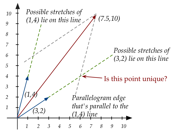
- Example: \(1.5(1,4) + 2(3,2)\)
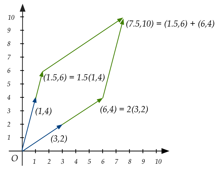
- Vector \((1,4)\) is stretched to \(1.5(1,4) = (1.5,6)\).
- Vector \((3,2)\) is stretched to \(2(3,2) = (6,4)\).
- The two stretched vectors are added: \((1.5,6) + (6,4) = (7.5,10)\).
- This simple little "combined" operation, as we
will see, turns out to be the heart of linear algebra.
In-Class Exercise 4:
Download LinCombExample.java
and DrawTool.java. Then, examine
the code in LinCombExample to see how vectors and arrows
are drawn. Then, draw the remaining arrows to complete the parallelogram.
In-Class Exercise 5:
Download LinCombExample2.java
(you already have DrawTool).
Write code to implement vector addition and scalar multiplication,
and test with the example in main().
Let's further explore linear combinations:
- A question: given three vectors, can the third always be
expressed as a linear combination of the first two?
- Related question: are the scalars unique?
- Let \({\bf u, v, z}\) be three vectors.
- Can we always find numbers \(\alpha, \beta\) such that
\(\alpha {\bf u} + \beta {\bf v} = {\bf z}\)?
- Are there multiple possibilities for \(\alpha, \beta\)?
In-Class Exercise 6:
Download LinCombExample3.java.
The double-for loop tries to systematically search over possible
values of \(\alpha, \beta\) to see if some combination will work.
Write code to see if the linear combination
\(\alpha {\bf u} + \beta {\bf v}\)
is approximately equal to \({\bf z}\).
In-Class Exercise 7:
Solve the above problem by hand: are there
values of \(\alpha, \beta\) such that
\(\alpha {\bf u} + \beta {\bf v} = {\bf z}\)
when \({\bf u}=(1,4)\), \({\bf v}=(3,2)\)
and \({\bf z}=(7.5,10)\)?
In-Class Exercise 8:
Suppose \({\bf u}=(1,2), {\bf v}=(3,6)\) and
\({\bf z}=(7.5,10)\). Download
LinCombExample4.java
and draw all three vectors. Then:
- Use the drawing to explain why no linear combination of
\({\bf u}\) and \({\bf v}\) will work.
- Solve by hand to confirm the explanation algebraically.
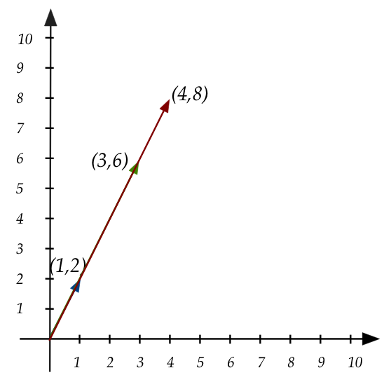
In-Class Exercise 9:
Now consider
\({\bf u}=(1,2), {\bf v}=(3,6)\) and
\({\bf z}=(4,8)\). Write code in
LinCombExample5.java
to draw these. Is there a unique solution? Explain both
geometrically and algebraically.
A linear combination can go beyond two vectors:
- Suppose \({\bf u}=(1,4), {\bf v}=(3,2), {\bf w}=(-1,1)\).
- If \(\alpha, \beta, \gamma\) are three numbers, then
\( \alpha{\bf u} + \beta{\bf v} + \gamma{\bf w}\) is
a linear combination.
- We often write a general linear combination of \(k\)
vectors as follows:
- Let \({\bf v}_1, {\bf v}_2, \ldots, {\bf v}_k\) be
\(k\) vectors.
- Let \(\alpha_1, \alpha_2, \ldots, \alpha_k\) be
\(k\) real numbers (the scalars).
- Then, \(\sum_{i=1}^k \alpha_i {\bf v}_i
= \alpha_1{\bf v}_1 + \ldots + \alpha_k{\bf v}_k \)
is a linear combination of the \(k\) vectors.
- Important: Notice the potential confusion in notation:
- We have been using \({\bf v} = (v_1,v_2,\ldots,v_n)\)
to describe a single vector.
- Here, \(v_i\) is a number, an element of the vector.
- But, above, \({\bf v}_1, {\bf v}_2, \ldots\) are vectors
in a collection of vectors.
- So, sometimes subscripts need to be parsed carefully.
In-Class Exercise 10:
Finally, consider
\({\bf u}=(1,4), {\bf v}=(3,2), {\bf w}=(-1,1)\) and
\({\bf z}=(7.5,10)\). We will ask whether there is a
linear combination
\(\alpha{\bf u} + \beta{\bf v} + \gamma{\bf w}\)
such that
\(\alpha{\bf u} + \beta{\bf v} + \gamma{\bf w} = {\bf z}\).
Write out the equations and explain algebraically
whether there is a solution.
The code in LinCombExample6.java
draws all four vectors. Can a linear combination of any two of
\({\bf u, v, w}\) suffice to produce \({\bf z}\)?
Next, let's examine a 3D example:
- Let \({\bf u}=(1,3,1), {\bf v}=(4,1,0), {\bf w}=(3,2,6)\)
and \({\bf z}=(1,7,8)\).
- We'd like to know if a linear combination of
\({\bf u,v,w}\) an produce \({\bf z}\).
- That is, can we find numbers \(\alpha, \beta, \gamma\)
such that
\(\alpha{\bf u} + \beta{\bf v} + \gamma{\bf w} = {\bf z}\)?
- With the above example, it would mean
$$
\alpha(1,3,1) + \beta (4,1,0) + \gamma (3,2,6) = (1,7,8)
$$
In-Class Exercise 11:
The code in LinComb3DExample.java
displays the vectors in the above example. (You need to have the Draw3D jar in
your CLASSPATH).
Write down the equations for \(\alpha, \beta, \gamma\)
and solve by hand.
In-Class Exercise 12:
Add code to LinComb3DExample2.java
to display the 3D version of the 2D parallelogram. That is,
draw arrows that show the stretched vectors when scaling
by \(\alpha, \beta, \gamma\) respectively. Then draw arrows
from the tips of the stretched vectors to the resultant
vector \({\bf z}\).
In-Class Exercise 13:
Suppose now that
\({\bf u}=(1,3,1), {\bf v}=(4,1,0), {\bf w}=(9,5,1)\) and
\({\bf z}=(1,7,8)\). We seek
\(\alpha, \beta, \gamma\) such that
\(\alpha{\bf u} + \beta{\bf v} + \gamma{\bf w} = {\bf z}\).
Write down the equations for \(\alpha,\beta,\gamma\) and
solve by hand.
The code in LinComb3DExample3.java
displays the four vectors.
Explain geometrically why this is consistent with your solution.
3.3
Vectors in column form
The column form:
- Earlier, we wrote vectors in "row" form, e.g.,
$$
{\bf u} \;\; = \;\; (4,1,0)
$$
- In column form, it looks like:
$$
{\bf u} \;\; = \;\; \vecthree{4}{1}{0}
$$
- The column form is generally preferred. At least, for
theoretical reasons, this is how you should think of it.
- Later, we will see that the row form is called
the transpose of the column form.
- Then, strictly speaking \({\bf u}^T \; = \; (4,1,0)\)
- Here, the superscript \({ }^T\) denotes transpose.
- For a vector, transpose means flipping from horizontal
to vertical or vice-versa.
- Thus,
$$
({\bf u}^T)^T \;\; = \;\; \vecthree{4}{1}{0}
$$
3.4
Matrices
To see where matrices come from, let's look at some earlier
examples with linear combinations
- Recall this 2D example: we seek \(\alpha, \beta\) such that
$$
\alpha (1,4) + \beta (3,2) \eql (7.5,10)
$$
- In column form, this becomes
$$
\alpha \vectwo{1}{4} + \beta \vectwo{3}{2} \eql \vectwo{7.5}{10}
$$
- In some sense, the \(\alpha\) and \(\beta\) are the two
items of interest, with the rest of numbers as the "data".
- Suppose we group the "data" as follows:
$$
\mat{
1 & 3\\
4 & 2\\}
\times
\rvectwo{\alpha}{\beta}
\eql
\vectwo{7.5}{10}
$$
- For the moment, we've put the linear
combination scalars \(\alpha\) and \(\beta\) in what looks
like a column vector.
- Similarly, let's consider a 3D example:
$$
\alpha (1,3,1) + \beta (4,1,0) + \gamma (3,2,6)
\eql (1,7,8)
$$
- In column form:
$$
\alpha \vecthree{1}{3}{1} + \beta \vecthree{4}{1}{0}
+ \gamma \vecthree{3}{2}{6}
\eql \vecthree{1}{7}{8}
$$
- As with the 2D case, we'll group the "data" and
multipliers (scalars) separately:
$$
\mat{
1 & 4 & 3\\
3 & 1 & 2\\
1 & 0 & 6\\
}
\times
\rvecthree{\alpha}{\beta}{\gamma}
\eql
\vecthree{1}{7}{8}
$$
- Once again, the linear combination
multipliers \(\alpha, \beta, \gamma\)
are grouped in what suspiciously looks like a vector but isn't. (Yet.)
- The larger, rectangular blocks like
$$
\mat{
1 & 3\\
4 & 2\\}
\;\;\; \mbox{ and } \;\;\;
\mat{
1 & 4 & 3\\
3 & 1 & 2\\
1 & 0 & 6\\
}
$$
are called matrices (matrix in singular form).
- Observe how the columns of the matrix are "peeled off"
to match the corresponding multiplier in the linear-combination.
- Example: in writing
$$
\mat{
\color{dkgreen}{1} & \color{dkred}{3} \color{black}{}\\
\color{dkgreen}{4} & \color{dkred}{2} \color{black}{}\\
}
\times
\rvectwo{\color{dkgreen}{\alpha}}{\color{dkred}{\beta}}
\color{black}{}
\eql
\vectwo{7.5}{10}
$$
we really mean
$$
\color{dkgreen}{\alpha} \color{black}{}
\mat{\color{dkgreen}{1}\\ \color{dkgreen}{4} \color{black}{}}
\; + \;
\color{dkred}{\beta} \color{black}{}
\mat{\color{dkred}{3} \\\color{dkred}{2} \color{black}{}}
\eql \vectwo{7.5}{10}
$$
- Similarly, in writing
$$
\mat{
\color{dkgreen}{1} & \color{dkred}{4} & \color{dkblue}{3} \color{black}{}\\
\color{dkgreen}{3} & \color{dkred}{1} & \color{dkblue}{2} \color{black}{}\\
\color{dkgreen}{1} & \color{dkred}{0} & \color{dkblue}{6} \color{black}{}\\
}
\times
\rvecthree{\color{dkgreen}{\alpha}}{\color{dkred}{\beta}}{\color{dkblue}{\gamma}} \color{black}{}
\eql
\vecthree{1}{7}{8}
$$
we really mean
$$
\color{dkgreen}{\alpha} \color{black}{}
\mat{\color{dkgreen}{1}\\ \color{dkgreen}{3} \\ \color{dkgreen}{1}
\color{black}{}}
\; + \;
\color{dkred}{\beta} \color{black}{}
\mat{\color{dkred}{4}\\ \color{dkred}{1} \\ \color{dkred}{0}
\color{black}{}}
\; + \;
\color{dkblue}{\gamma} \color{black}{}
\mat{\color{dkblue}{3}\\ \color{dkblue}{2} \\ \color{dkblue}{6}
\color{black}{}}
\eql \vecthree{1}{7}{8}
$$
- Now, notice how easy it is to "read off" the equations
for the multipliers from the linear-combination form:
\(\rhd\)
Simply multiply a row by the multipliers and equate to the
corresponding entry on the right side.
- Thus, for the first equation, we read if off from
$$
\color{dkgreen}{\bf \alpha} \color{black}{}
\mat{\color{dkgreen}{\bf 1}\\ \color{dkgreen}{3} \\ \color{dkgreen}{1}
\color{black}{}}
\; + \;
\color{dkred}{\bf \beta} \color{black}{}
\mat{\color{dkred}{\bf 4}\\ \color{dkred}{1} \\ \color{dkred}{0}
\color{black}{}}
\; + \;
\color{dkblue}{\bf \gamma} \color{black}{}
\mat{\color{dkblue}{\bf 3}\\ \color{dkblue}{2} \\ \color{dkblue}{6}
\color{black}{}}
\eql \vecthree{\bf 1}{7}{8}
$$
to get
$$
\color{dkgreen}{\bf \alpha \times 1} \color{black}{}
+
\color{dkred}{\bf \beta \times 4} \color{black}{}
+
\color{dkblue}{\bf \gamma \times 3} \color{black}{}
\eql
{\bf 1}
$$
- It's a bit harder to read it off from the matrix form,
but you get used to it:
$$
\mat{
\color{dkgreen}{\bf 1} & \color{dkred}{\bf 4} &
\color{dkblue}{\bf 3} \color{black}{}\\
\color{dkgreen}{3} & \color{dkred}{1} & \color{dkblue}{2} \color{black}{}\\
\color{dkgreen}{1} & \color{dkred}{0} & \color{dkblue}{6} \color{black}{}\\
}
\times
\rvecthree{\color{dkgreen}{\alpha}}{\color{dkred}{\beta}}{\color{dkblue}{\gamma}} \color{black}{}
\eql
\vecthree{\bf 1}{7}{8}
$$
- So, a matrix is really a collection of (column) vectors.
3.5
The matrix vector equation
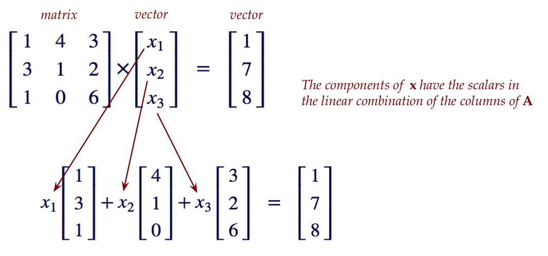
Let's go back to the 3D example above:
$$
\mat{
1 & 4 & 3\\
3 & 1 & 2\\
1 & 0 & 6\\
}
\times
\rvecthree{\alpha}{\beta}{\gamma}
\eql
\vecthree{1}{7}{8}
$$
- As mentioned, the grouping of the multipliers
\(\alpha, \beta, \gamma\) looks suspiciously like a vector.
- One could develop a reasonable theory of linear algebra
treating this grouping as a "collection of multipliers"
but NOT as a vector.
- However, we will take a leap of faith right now and
simply put the multipliers into a vector (notice the square brackets):
$$
\mat{
1 & 4 & 3\\
3 & 1 & 2\\
1 & 0 & 6\\
}
\times
\vecthree{\alpha}{\beta}{\gamma}
\eql
\vecthree{1}{7}{8}
$$
- Are we allowed to do this?
- The three numbers are just that: numbers.
- The grouping is therefore a tuple.
- Which means we could treat it as a vector (and get
away with it).
- Of course, at this point, we don't know if it makes
geometrical sense to do so.
- Because it's now a vector, we will use a single symbol
with subscripts:
$$
\mat{
1 & 4 & 3\\
3 & 1 & 2\\
1 & 0 & 6\\
}
\times
\vecthree{x_1}{x_2}{x_3}
\eql
\vecthree{1}{7}{8}
$$
-
Thus, the multipliers are now called \(x_1, x_2\) and \(x_3\).
\(\rhd\)
They are elements of the vector \({\bf x}=(x_1, x_2, x_3)\).
- We will also name the vector on the right side:
$$
{\bf b} = \vecthree{1}{7}{8}
$$
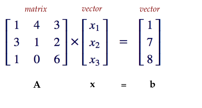
- Lastly, we will also use a boldface symbol for the matrix itself, for example:
$$
{\bf A} \eql
\mat{
1 & 4 & 3\\
3 & 1 & 2\\
1 & 0 & 6\\
}
$$
- Finally, we are in a position to write the linear
combination in its most compact form:
$$
{\bf A x} \eql {\bf b}
$$
- Let's consider what it would look like for larger
matrices:
- An \(n \times n\) matrix \({\bf A}\) is often written
as the following, with \(a_{ij}\) denoting the entry
(a number) in row \(i\) and column \(j\):
$$
\mat{
a_{11} & a_{12} & \cdots & a_{1n} \\
a_{21} & a_{22} & \cdots & a_{2n} \\
\vdots & \vdots & & \vdots \\
a_{n1} & a_{n2} & \cdots & a_{nn} \\
}
$$
- Then, the product with a vector \({\bf x}\) of length \(n\)
looks like:
$$
\mat{
a_{11} & a_{12} & \cdots & a_{1n} \\
a_{21} & a_{22} & \cdots & a_{2n} \\
\vdots & \vdots & & \vdots \\
a_{n1} & a_{n2} & \cdots & a_{nn}
}
\mat{
x_1\\
x_2\\
\vdots\\
x_n
}
$$
- The result is a vector:
$$
\mat{
a_{11} & a_{12} & \cdots & a_{1n} \\
a_{21} & a_{22} & \cdots & a_{2n} \\
\vdots & \vdots & & \vdots \\
a_{n1} & a_{n2} & \cdots & a_{nn}
}
\mat{
x_1\\
x_2\\
\vdots\\
x_n
}
\eql
\mat{
\sum_{k=1}^n a_{1k} x_k\\
\sum_{k=1}^n a_{2k} x_k\\
\vdots\\
\sum_{k=1}^n a_{nk} x_k
}
$$
Observe: each sum on the right is a single number.
In-Class Exercise 14:
Apply the matrix
\({\bf A}=\mat{a_{11} & a_{12}\\ a_{21} & a_{22}}\) to the vector
\({\bf x}=\vectwo{x_1}{x_2}\). What are the dimensions (number of
rows, number of columns) of the
resulting product?
The two fundamental interpretations of the
matrix-vector equation \({\bf A x} = {\bf b}\):
- Interpretation as a linear combination of columns of \({\bf A}\):
- Here, the elements of \({\bf x}\) are merely multipliers.
- \({\bf x}\) is not treated as a vector, except for the
convenience of writing.
- We are commonly given \({\bf b}\) (and \({\bf A}\)),
and wish to solve for \({\bf x}\).
- Interpretation as a matrix "acting" on a vector (or
transforming it):
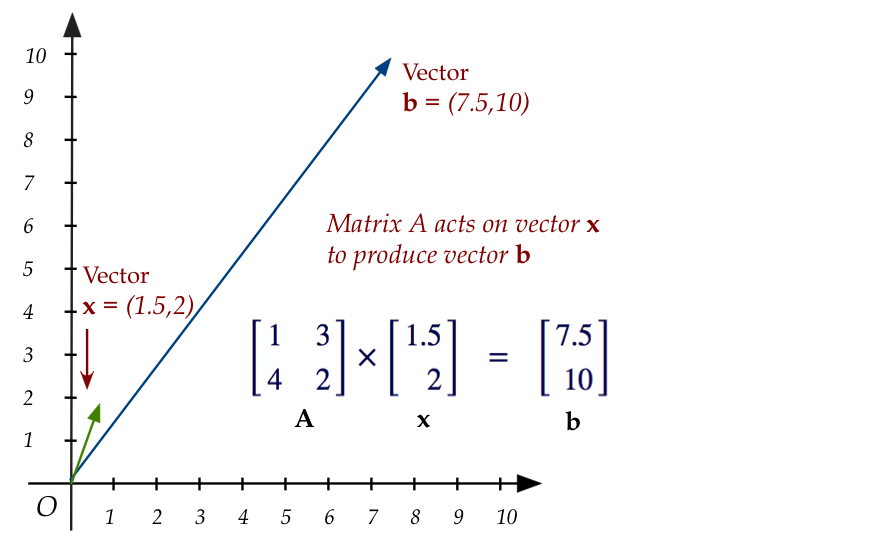
- Here, \({\bf x}\) is treated as a vector.
- The matrix "does something to it" through multiplication,
producing the vector \({\bf b}\) on the right.
- Thus, the matrix \({\bf A}\) can be said to transform
vector \({\bf x}\) into vector \({\bf b}\).
- With this interpretation \({\bf A x} = {\bf b}\) is
not so much an equation as a generating formula:
we are given \({\bf A}\) and \({\bf x}\) to compute \({\bf b}\).
The latter interpretation turns out to both greatly expand
the interesting theory and useful applications of linear algebra.
In-Class Exercise 15:
Apply the matrix
\({\bf A}=\mat{2 & -3\\ 0 & 1}\) to the vector \({\bf
x}=\vectwo{2}{3}\) to get the vector \({\bf y}\).
Then apply \({\bf B}=\mat{1 & 2\\ 0 & -3}\) to \({\bf y}\) to
get \({\bf z}\).
What are \({\bf y}\) and \({\bf z}\)?
Show your calculations.
In-Class Exercise 16:
Download MatrixVectorExample.java
and write code to perform the matrix-vector product. Then
confirm your calculations above from the displayed vectors.
In-Class Exercise 17:
Compute the vector obtained by multiplying \({\bf x}\)
above by the matrix \({\bf C} = \mat{2 & -1\\ 0 & -3}\).
Compare with the value of \({\bf z}\) calculated earlier.
In-Class Exercise 18:
Compute the vector obtained by multiplying \({\bf z}\)
above by the matrix \({\bf C}_2 = \mat{1.0/2 & -1.0/6\\ 0 & -1.0/3}\).
Compare with the value of \({\bf x}\) calculated earlier.
In-Class Exercise 19:
Earlier, you computed the product of
\({\bf A}=\mat{a_{11} & a_{12}\\ a_{21} & a_{22}}\) with the vector
\({\bf x}=\vectwo{x_1}{x_2}\), which produces a result vector.
Multiply this result vector by
\({\bf B}=\mat{b_{11} & b_{12}\\ b_{21} & b_{22}}\).
(The result is admittedly not pretty.)
Finally, note that matrices need not be square:
$$
\mat{
1 & 4 & 3 & 0 & 5\\
3 & 1 & 2 & -1.5 & 5\\
1 & 0 & 6 & -2 & 1\\
}
\times
\mat{ x_1 \\ x_2 \\ x_3 \\ x_4 \\ x_5}
\eql
x_1 \vecthree{1}{3}{1} + x_2 \vecthree{4}{1}{0}
+ x_3 \vecthree{3}{2}{6}
+ x_4 \vecthree{0}{-1.5}{-2}
+ x_5 \vecthree{5}{5}{1}
\eql
\mat{ b_1 \\ b_2 \\ b_3}
$$
- Here, the 5 columns of the matrix are 3-component vectors.
- A linear combination of the 5 columns needs 5 multipliers:
\(x_1, x_2, x_3, x_4, x_5\).
- The linear combination results in a 3-component vector,
which we have called \({\bf b}=(b_1,b_2,b_3)\).
- Thus, a matrix with \(m\) rows and \(n\) columns is
multiply-compatible with a vector that has
\(n\) components, resulting in a vector with \(m\) components.
- We write this as
$$
{\bf A}_{m\times n} {\bf x}_{n\times 1} \eql {\bf b}_{m\times 1}
$$
3.6
Matrix-matrix multiplication
Consider the following example of a matrix \({\bf A}\)
multiplying (and thus transforming) a vector \({\bf x}\):
$$
{\bf Ax} \eql
\mat{2 & -3\\ 0 & 1} \vectwo{2}{3}
$$
Suppose the result is the vector \({\bf y}\):
$$
\mat{2 & -3\\ 0 & 1} \vectwo{2}{3}
\eql
\vectwo{y_1}{y_2}
$$
Now suppose we multiply \({\bf y}\) by the matrix \({\bf B}\)
to get the vector \({\bf z}\):
$$
\mat{1 & 2\\ 0 & -3} \vectwo{y_1}{y_2}
\eql
\vectwo{z_1}{z_2}
$$
But because \({\bf y}\) is itself created from the matrix-vector
product \({\bf Ax}\), we can replace \({\bf y}\) with
$$
\mat{1 & 2\\ 0 & -3} \left( \mat{2 & -3\\ 0 & 1} \vectwo{2}{3} \right)
\eql
\vectwo{z_1}{z_2}
$$
Obviously, the interesting question is whether the two
matrices can be "combined" to create a single matrix to
transform \({\bf x}=(2,3)\) into \({\bf z}\):
$$
\color{dkgreen}{
\mat{1 & 2\\ 0 & -3} \mat{2 & -3\\ 0 & 1}
} \color{black}{} \vectwo{2}{3}
\eql
\color{dkgreen}{\mat{? & ?\\ ? & ?}}
\color{black}{} \vectwo{2}{3}
\eql
\vectwo{z_1}{z_2}
$$
As it turns out, there is a nice way to "multiply" matrices
so that the resulting product produces the same action as
the two original matrices applied in succession.
Let's work this out for the \(2\times 2\) case:
$$
\eqb{
\mat{b_{11} & b_{12}\\ b_{21} & b_{22}}
\mat{a_{11} & a_{12}\\ a_{21} & a_{22}}
\vectwo{x_1}{x_2}
& \eql &
\mat{b_{11} & b_{12}\\ b_{21} & b_{22}}
\mat{a_{11}x_1 + a_{12}x_2 \\ a_{21}x_1 + a_{22}x_2}\\
& \eql &
\mat{
b_{11}(a_{11}x_1 + a_{12}x_2) + b_{12} (a_{21}x_1 + a_{22}x_2)\\
b_{21}(a_{11}x_1 + a_{12}x_2) + b_{22} (a_{21}x_1 + a_{22}x_2)
}\\
& \eql &
\mat{
(b_{11}a_{11} + b_{12}a_{21})x_1
+ (b_{11}a_{12} + b_{12}a_{22})x_2 \\
(b_{21}a_{11} + b_{22}a_{21})x_1
+ (b_{21}a_{12}+ b_{22}a_{22})x_2
}\\
& \eql &
\mat{
b_{11}a_{11} + b_{12}a_{21} &
b_{11}a_{12} + b_{12}a_{22} \\
b_{21}a_{11} + b_{22}a_{21} &
b_{21}a_{12}+ b_{22}a_{22}
}
\vectwo{x_1}{x_2}
}
$$
And so, we have the matrix-matrix product
$$
\mat{b_{11} & b_{12}\\ b_{21} & b_{22}}
\mat{a_{11} & a_{12}\\ a_{21} & a_{22}}
\eql
\mat{
b_{11}a_{11} + b_{12}a_{21} &
b_{11}a_{12} + b_{12}a_{22} \\
b_{21}a_{11} + b_{22}a_{21} &
b_{21}a_{12}+ b_{22}a_{22}
}
$$
Notice that each entry of the result happens to be a row of \({\bf B}\)
times a column of \({\bf A}\)
And it happens to generalize to larger matrices:
- Suppose we multiply matrices \({\bf B}\) and \({\bf A}\)
to get \({\bf C}\):
$$
\mat{
b_{11} & b_{12} & \cdots & b_{1n} \\
b_{21} & b_{22} & \cdots & b_{2n} \\
\vdots & \vdots & & \vdots \\
b_{n1} & b_{n2} & \cdots & b_{nn}
}
\mat{
a_{11} & a_{12} & \cdots & a_{1n} \\
a_{21} & a_{22} & \cdots & a_{2n} \\
\vdots & \vdots & & \vdots \\
a_{n1} & a_{n2} & \cdots & a_{nn}
}
\eql
\mat{
c_{11} & c_{12} & \cdots & c_{1n} \\
c_{21} & c_{22} & \cdots & c_{2n} \\
\vdots & \vdots & & \vdots \\
c_{n1} & c_{n2} & \cdots & c_{nn}
}
$$
- Then, element \(c_{ij}\) is the product of
the \(i^{th}\) row of \({\bf B}\) and the \(j^{th}\) column
of \({\bf A}\).
$$
c_{ij} \eql \sum_{k=1}^n b_{ik} a_{kj}
$$
In-Class Exercise 20:
Download MatrixVectorExample2.java
and write matrix multiplication code to make the example work.
Confirm that you obtained the same matrix in Exercise 17, and the
same resulting vector.
In-Class Exercise 21:
Consider the matrices
$$
{\bf A} \; = \;
\mat{
3 & 2 & 1\\
-2 & 3 & 5\\
0 & 0 & 3
}
\;\;\;\;\;\;\;
\mbox{ and }
\;\;\;\;\;\;\;
{\bf B} \; = \;
\mat{
-4 & 1 & 0\\
1 & 0 & 1\\
3 & -2 & 1
}
$$
Let \({\bf x}=(1,-1,2)\) and define \({\bf y}={\bf Ax}\) and
\({\bf z}={\bf By}\). Calculate each of \({\bf y, z}\) and
the matrix product \({\bf C}={\bf BA}\). Confirm by calculating
\({\bf Cx}\).
In-Class Exercise 22:
Download MatrixVector3DExample.java,
then fill in the code (from previous exercises) to perform matrix
multiplication and matrix-vector multiplication.
Confirm that the results match the calculations in the previous exercise.
In-Class Exercise 23:
Suppose \({\bf A}\) and \({\bf B}\) are two \(n \times n\) matrices.
Prove or disprove: \({\bf AB} = {\bf BA}\).
3.7
Non-square matrices
Because the matrix multiplication takes a row from the left
matrix and multiplies into a column of the right matrix,
it turns out we can multiply non-square matrices:
- Example:
- Suppose
$$
{\bf A} \eql
\mat{
1 & 0 & -1 & 2 & 0\\
0 & 2 & -3 & 1 & 3
}
\;\;\;\;\;\;\;\; \mbox{ and } \;\;\;\;\;\;\;\;
{\bf B} \eql
\mat{
-1 & 2 & 0\\
4 & 0 & -2\\
0 & -2 & 1\\
-1 & 1 & 3\\
5 & -2 & -1
}
$$
- Then \({\bf AB}\) can be computed as
$$
{\bf AB} \eql
\mat{
1 & 0 & -1 & 2 & 0\\
0 & 2 & -3 & 1 & 3
}
\mat{
-1 & 2 & 0\\
4 & 0 & -2\\
0 & -2 & 1\\
-1 & 1 & 3\\
5 & -2 & -1
}
\eql
\mat{
-3 & 6 & 5\\
22 & 1 & -7
}
$$
- They are multiple-compatible because a row of \({\bf A}\)
has the same number of elements as a column of \({\bf B}\).
- Each row of \({\bf A}\) (there are 2 of them)
multiplies each column of \({\bf B}\) (3 of them)
\(\rhd\)
There will be \(2 \times 3\) entries for a \(2 \times 3\)
matrix.
- Notation: we often write \({\bf A}_{m\times n}\) to
explicitly note the number of rows (\(m\)) and columns (\(n\)).
- Thus, \({\bf C}_{m\times k} = {\bf A}_{m\times n} {\bf
B}_{n\times k}\)
- Here, \({\bf A}_{m\times n}\) and \({\bf B}_{n\times k}\)
are multiply-compatible.
- The result matrix is \(m \times k\).
- Notation: for any matrix \({\bf A}\), the entry in the
i-th row and j-th column is sometimes referred to as
\({\bf A}_{ij}\) or \({\bf A}(i,j)\).
In-Class Exercise 24:
What is the result of multiplying
\({\bf A} = \mat{0 & 1 & 0\\ -1 & 2 & 0}\)
and
\({\bf B}= \mat{ 1 & 1\\ 2 & 2\\ 0 & -3}\)?
What is \({\bf Ax}\) when \({\bf x}=(2,3,4)\)?
3.8
A review of three cases involving equations
Let's revisit three types of situations we encountered when
solving equations:
- Problem 1:
$$
\eqb{
x_1 + 3x_2 & = 7.5 \\
4x_1 + 2x_2 & = 10 \\
}
$$
- Problem 2
$$
\eqb{
x_1 + 3x_2 & = 7.5 \\
2x_1 + 6x_2 & = 10 \\
}
$$
- Problem 3
$$
\eqb{
x_1 + 3x_2 & = 4 \\
2x_1 + 6x_2 & = 8 \\
}
$$
Problem 1:
- The first set of equations is:
$$
\eqb{
x_1 + 3x_2 & = 7.5 \\
4x_1 + 2x_2 & = 10 \\
}
$$
Which in matrix form is:
$$
\mat{
1 & 3\\
4 & 2\\}
\vectwo{x_1}{x_2}
\eql
\vectwo{7.5}{10}
$$
- Let's now write the same in "vector stretch" form:
$$
x_1 \vectwo{1}{4} + x_2 \vectwo{3}{2} \eql \vectwo{7.5}{10}
$$
- The solution is: \(x_1=1.5, \;\; x_2=2\).
- Pictorially:
- Thus, we can see clearly that there exists one linear
combination of the two vectors \((1,4)\) and \((3,2)\) that produces \((7.5,10)\).
Problem 2:
- The second set of equations
$$
\eqb{
x_1 + 3x_2 & = 7.5 \\
2x_1 + 6x_2 & = 10 \\
}
$$
in "vector stretch" form:
$$
x_1 \vectwo{1}{2} + x_2 \vectwo{3}{6} \eql \vectwo{7.5}{10}
$$
- The solution? There is no solution.
- Pictorially:
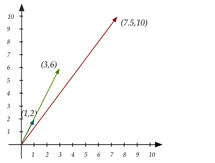
- Clearly, no linear combination of
\((1,2)\) and \((3,6)\) produces \((7.5,10)\).
- In fact, all linear combinations of
\((1,2)\) and \((3,6)\) lie on the line that both fall on.
- Which means they could not linearly combine to form a vector
at any other angle.
- Thus, without trying you can tell that these equations do
not have a solution:
$$
\eqb{
x_1 + 3x_2 & = 4 \\
2x_1 + 6x_2 & = 3 \\
}
$$
Problem 3:
- The third set
$$
\eqb{
x_1 + 3x_2 & = 4 \\
2x_1 + 6x_2 & = 8 \\
}
$$
in "vector stretch" form:
$$
x_1 \vectwo{1}{2} + x_2 \vectwo{3}{6} \eql \vectwo{4}{8}
$$
- The solution? There are infinitely many solutions.
- Pictorially:
- Is it obvious from the picture that there are infinitely
many solutions?
A few more observations and questions:
- Let's return to the picture in Problem 1:
- The picture illustrates why, in this case, the solution is unique.
- Some questions that arise at this point:
- Are these the only three possible cases for any set of equations?
- When multiple solutions exist, is it always an infinite
number of them?
- When there's a unique solution, does it always correspond to
a picture like the one above?
3.9
Study tips
- This module contains many important seed ideas. It's worth
reviewing carefully.
- When you read, read with pen-and-paper and work on the
exercises as you go, NOT at the end of reading it all.
- Even though some of the solve-by-hand examples are a bit
tedious, they are worth doing at least once because they help
drive home a definition or procedure.
- Write down a summary or list of highlights for each module.
One important learning goal in any course should be to build an
internal narrative of how different pieces of course
fit together.
At this early stage, we don't have enough "pieces" to form
an idea of the whole.
Since this is a theoretical course, a good thing to do is
to keep note of interesting theoretical questions along the way.
In this module, some of the questions that come to mind:
- Given two vectors \({\bf u,v}\), under what conditions
is it possible
to express any other vector \({\bf w}\) as a linear combination
of the two?
- Does an answer to this question depend on the dimension?
- In general, do observations about 2D and 3D generalize to \(n\)
dimensions?
- What properties of regular (number to number) multiplication
are also satisfied by matrix multiplication?
- If a matrix \({\bf A}\) transforms a vector \({\bf x}\)
into \({\bf b}={\bf Ax}\), is it possible to find
a matrix \({\bf A'}\) to reverse the transformation, i.e,
\({\bf x}={\bf A'b}\)?