Module objectives
By the end of this module, you should be able to
- Explain the terms: spectral theorem, diagonalization,
eigenbasis.
- Understand how Principal Component Analysis (PCA) works,
and its relation to the spectral theorem.
12.0
A review of some ideas
Let's list a few results and definitions that will be useful in this
module, some we've seen before and some new:
- How to write the matrix product \({\bf AB}\) in terms
of the columns of \({\bf B}\).
- How to change coordinates from one basis to another.
- How to write multiple eigenvector-eigenvalue pairs in matrix form.
- How to permute the columns in this matrix form.
- The inverse of an orthogonal matrix.
- The product of a single-column matrix (a vector) and a
single-row matrix (a transposed vector) is a matrix.
- The outerproduct form of matrix multiplication.
- A definition: symmetric matrix
Important: It's highly recommended that, as you proceed below,
to write these down and review them before proceeding with further
sections in this module.
Useful fact #1: the product \({\bf AB}\) can be written in
terms of the columns of \({\bf B}\) as
$$
{\bf AB} \eql
{\bf A}
\mat{ & & & \\
\vdots & \vdots & \vdots & \vdots\\
{\bf b}_1 & {\bf b}_2 & \cdots & {\bf b}_n\\
\vdots & \vdots & \vdots & \vdots\\
& & &
}
\eql
\mat{ & & & \\
\vdots & \vdots & \vdots & \vdots\\
{\bf A b}_1 & {\bf A b}_2 & \cdots & {\bf A b}_n\\
\vdots & \vdots & \vdots & \vdots\\
& & &
}
$$
That is, we stack the individual \({\bf A b}_i\) products (which
are vectors) as columns in the result.
- Let's see how this works in an example. Consider
$$
{\bf A B} \eql
\mat{1 & 2\\ 0 & -3} \mat{\color{dkgreen}{2} & \color{blue}{-3}\\ \color{dkgreen}{0} & \color{blue}{1}}
\eql
\mat{\color{dkgreen}{2} & \color{blue}{-1}\\ \color{dkgreen}{0} & \color{blue}{-3}}
$$
- The first column on the right becomes
$$
{\bf A b}_1 \eql
\mat{1 & 2\\ 0 & -3} \mat{\color{dkgreen}{2} \\ \color{dkgreen}{0}}
\eql
\mat{\color{dkgreen}{2} \\ \color{dkgreen}{0} }
$$
The second column becomes
$$
{\bf A b}_2 \eql
\mat{1 & 2\\ 0 & -3} \mat{\color{blue}{-3}\\ \color{blue}{1}}
\eql
\mat{\color{blue}{-1}\\ \color{blue}{-3}}
$$
- See Module 4 for the proof.
Useful result #2: change of coordinates
- The problem is this:
- Suppose \({\bf v}\) is a vector in the standard basis.
- Suppose \({\bf x}_1,{\bf x}_2,\ldots,{\bf x}_n\) is another
basis.
- We want the coordinates of the vector \({\bf v}\) in
this second basis.
- Recall the meaning of coordinates:
- If \({\bf v}=(v_1,v_2,\ldots,v_n)\) then
$$
{\bf v} \eql
v_1 \vecfour{1}{0}{\vdots}{0}
+
v_2 \vecfour{0}{1}{\vdots}{0}
+ \ldots
+ v_n \vecfour{0}{0}{\vdots}{1}
\eql
v_1 {\bf e}_1 + v_2{\bf e}_2 + \ldots + v_n{\bf e}_n
$$
- Thus, the vector \({\bf v}\)'s coordinates are the
coefficients of the linear combination used to
construct \({\bf v}\) using the standard basis vectors.
- To get the same vector's coordinates in another basis,
we need to ask: what linear combination of the new basis
vectors will produce the same vector?
- Thus, if the basis consists of the vectors
\({\bf x}_1,{\bf x}_2,\ldots,{\bf x}_n\),
we want to find \(\alpha_1,\alpha_2,\ldots,\alpha_n\) such that
$$
{\bf v} \eql \alpha_1 {\bf x}_1 + \alpha_2 {\bf x}_2
+ \ldots + \alpha_n {\bf x}_n
$$
- Once we find such \(\alpha_i\)'s, then the
coordinates are: \((\alpha_1,\alpha_2,\ldots,\alpha_n)\)
- Which we can write in vector form as:
$$
{\bf u} \eql (\alpha_1,\alpha_2,\ldots,\alpha_n)
$$
- To find the \(\alpha_i\)'s
- Write the linear combination in matrix form:
$$
{\bf v} \eql \alpha_1 {\bf x}_1 + \alpha_2 {\bf x}_2
+ \ldots + \alpha_n {\bf x}_n
\eql
\mat{ & & & \\
\vdots & \vdots & \vdots & \vdots\\
{\bf x}_1 & {\bf x}_2 & \cdots & {\bf x}_n\\
\vdots & \vdots & \vdots & \vdots\\
& & &
}
\mat{\alpha_1\\ \alpha_2 \\ \vdots \\ \alpha_n}
$$
- Let's name the matrix above \({\bf X}\).
- Then, we've written
$$
{\bf v} \eql {\bf X u}
$$
- And so,
$$
{\bf u} \eql {\bf X}^{-1} {\bf v}
$$
- Thus, the procedure is:
- Create a matrix with the new basis vectors as columns.
- Invert the matrix.
- Multiply into old coordinates.
This is exactly what we did in Module 4.
Useful fact #3: writing eigenvector-eigenvalue pairs in matrix form.
Useful fact #4:
If \({\bf S}\) has an inverse, then we can right-multiply
both sides
$$
{\bf A S} {\bf S}^{-1} \eql {\bf S \Lambda} {\bf S}^{-1}
$$
to get
$$
{\bf A} \eql {\bf S \Lambda} {\bf S}^{-1}
$$
which is a decomposition that expresses a matrix \({\bf A}\) in terms
of its eigenvectors and eigenvalues. This will shortly turn out to
be quite useful.
Useful fact #5:
If we permute the columns of \({\bf S}\) above, the relation
$$
{\bf A S} \eql {\bf S \Lambda}
$$
holds as long as the columns of \({\bf \Lambda}\) are permuted the
same way:
- For example, suppose we swap the first and third columns of
\({\bf S}\) and \({\bf \Lambda}\) above:
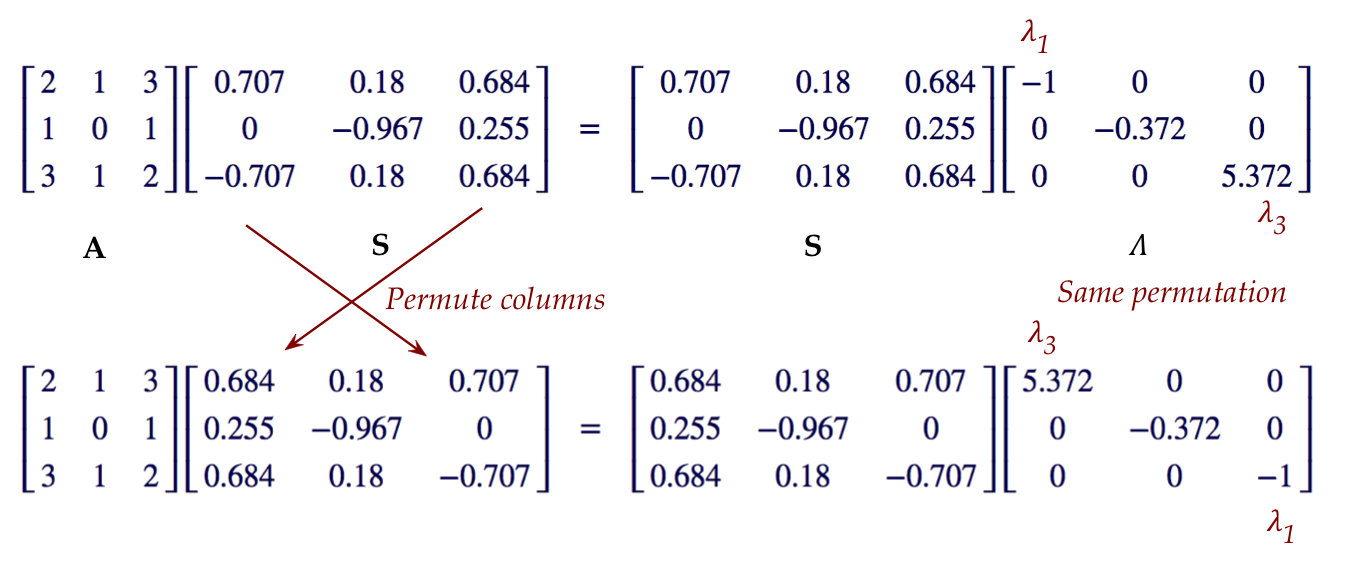
- This is going to be useful when we order the columns in
decreasing order of eigenvalues.
Useful fact #6:
recall that, for an orthogonal matrix \({\bf S}\)
- The columns are pairwise orthonormal.
- \({\bf S}^{-1} = {\bf S}^T\)
Useful fact #7: The product of a column times a row is a matrix
- Suppose \({\bf A}_{m\times k}\) and \({\bf B}_{k\times n}\)
are two multiply-compatible matrices.
- Then \({\bf C}={\bf AB}\) has dimensions \(m\times n\).
In-Class Exercise 2:
What are the dimension of \({\bf C}\) when
\({\bf A}\) is \(m\times 1\) and \({\bf B}\) is \(1\times n\)?
Create an example with \(m=3\) and \(n=4\).
- Another way of writing this:
- Suppose \({\bf u}\) and \({\bf v}\) are m-dimensional
and n-dimensional vectors.
- Then the product
$$
{\bf u} {\bf v}^T
$$
has dimensions \(m\times n\).
- Thus, the product of a column-vector times a row-vector (the
transpose) is a matrix!
- For example:
$$
\vecthree{1}{2}{3}
\mat{0 & -1 & 2}
\eql
\mat{0 & -1 & 2\\
0 & -2 & 4\\
0 & -3 & 6}
$$
In-Class Exercise 3:
Suppose \({\bf a}_m\) is the vector
\({\bf a}_m=(1,1,\ldots,1)\) with \(m\) 1's.
Calculate
\({\bf a}_4 {\bf a}_4^T + 2 {\bf a}_4 {\bf a}_4^T + 3 {\bf a}_4 {\bf a}_4^T\).
(Here m=n.)
Useful fact #8: The outerproduct form of matrix multiplication:
Useful definition (#9):
A symmetric matrix is a matrix \({\bf A}\) such that:
\({\bf A}^T = {\bf A}\).
- First, notice that a symmetric matrix is necessarily square.
- An example:
$$
\mat{
1 & 2 & 3 & 4\\
2 & 5 & 6 & 7\\
3 & 6 & 8 & 9\\
4 & 7 & 9 & 10
}
$$
12.1
Eigentheory
In-Class Exercise 5:
Suppose \({\bf A}\) is a \(2\times 2\) rotation matrix that
rotates a vector by \(45^\circ\).
Explain why there cannot be a nonzero vector \({\bf x}\) and real number
\(\lambda\) such that
\( {\bf Ax}= \lambda {\bf x}\).
It turns out that rotation matrices do have complex
eigenvalues and complex eigenvectors.
That is, we can find \(\lambda, {\bf x}\) such that
\( {\bf Ax}= \lambda {\bf x}\), where
\(\lambda\) is a complex number and
\({\bf x}\) is a complex vector.
About the theory relating to eigenvectors:
- Unfortunately, very little of the theory of eigenvectors is
simple.
- We will omit the theory because we want to get to the
practical part: symmetric matrices.
- Let's however summarize a few key results.
Existence of eigenvalues:
- Generally, most matrices have eigenvalues, if we allow
complex eigenvalues and eigenvectors.
- Proving this is not straightforward.
- There are at least a couple different approaches:
- One approach: use the characteristic polynomial
- Every matrix has an associated polynomial \(p(\lambda)\)
where \(p(\lambda)=0\) if and only if \(\lambda\) is an eigenvalue.
- Example:
$$
p(\lambda) \eql \lambda^3 - 3\lambda + 2
$$
- Furthermore, \(p(\lambda)\) is of degree \(n\)
for an \(n\times n\) matrix.
- The theory of determinants is used to define and prove
the above result.
- The Fundamental Theorem of Algebra implies that \(p(\lambda)=0\)
has \(n\) complex roots if the degree is \(n\).
- Some of the complex roots can be real (the imaginary part
happens to be zero).
Multiplicity:
- The characteristic polynomial also provides another
fundamental insight: potential multiplicity of eigenvalues
- For example
$$\eqb{
p(\lambda) & \eql & \lambda^3 - 3\lambda + 2\\
& \eql &
(\lambda - 1) (\lambda - 1) (\lambda - 2)
}$$
- There are three roots:
$$\eqb{
\lambda_1 & \eql & 1\\
\lambda_2 & \eql & 1\\
\lambda_3 & \eql & 2\\
}$$
- We usually say there are two eigenvalues, one
of which has a multiplicity of two.
An important result for real symmetric matrices:
- Recall: a matrix \({\bf A}\) is symmetric if
\({\bf A}^T = {\bf A}\).
- We'll first state the result and then explain.
- Theorem 12.1:
If \({\bf A}_{n\times n}\) is a real symmetric matrix then
- All its eigenvalues \(\lambda_1,\lambda_2,\ldots,\lambda_n\)
(with possible multiplicities) are real.
- There exist \(n\) corresponding
eigenvectors \({\bf x}_1,{\bf x}_2,\ldots,{\bf x}_n\)
such that the matrix
$$
{\bf S}
\defn
\mat{ & & & \\
\vdots & \vdots & \vdots & \vdots\\
{\bf x}_1 & {\bf x}_2 & \cdots & {\bf x}_n\\
\vdots & \vdots & \vdots & \vdots\\
& & &
}
$$
is orthogonal (the columns are orthonormal).
- This is not at all obvious, nor easy to prove.
(See the book by Olver & Shakiban)
- But let's understand what it's saying.
- We know the matrix \({\bf A}\) will have \(n\)
eigenvalues.
\(\rhd\)
This comes from the theory described above.
- But could some of them be complex?
- Theorem 12.1 says, however, that all will be real.
- Now one could believe that for distinct eigenvalues,
the corresponding eigenvectors will be different.
- What the theorem in fact says is:
- Suppose \(\lambda_i=\lambda_j\) is a multiplicity.
- That is, two eigenvalues that happen to be the same.
- Then, one can actually find two different and orthonormal
eigenvectors for these two eigenvalues.
- The method for finding these eigenvectors
is a bit involved, and won't be covered in this course.
In-Class Exercise 6:
Download SymmetricExample.java,
which computes the eigenvalues and eigenvectors for an example matrix. Verify that the
columns of \({\bf S}\) are orthogonal.
Applications of eigentheory:
- Our main goal in this module is to get to an important technique in
machine learning: principal component analysis (PCA)
- For this purpose we will need the spectral theorem (next).
- Note: eigenvalues and vectors have important applications in
physics and engineering, for example:
- The solution to certain types of differential equations.
- The solution to some kinds of recurrence relations.
- Circuit analysis.
- Perhaps the most important application of all is the
singular value decomposition (SVD), which we will study
in the next module.
12.2
The spectral theorem for real symmetric matrices
Our main goal in this module is to get a different type
of decomposition for real symmetric matrices: one
that involves eigenvectors.
Let's work our way towards the spectral theorem:
- From Theorem 12.1, a symmetric matrix \({\bf A}_{n\times n}\)
has \(n\) eigenvalues (with possible duplicates amongst them),
and \(n\) corresponding orthonormal eigenvectors
\({\bf x}_1,{\bf x}_2,\ldots,{\bf x}_n\).
- As we've done before, let's put the eigenvectors into a
matrix:
$$
{\bf S}
\eql
\mat{ & & & \\
\vdots & \vdots & \vdots & \vdots\\
{\bf x}_1 & {\bf x}_2 & \cdots & {\bf x}_n\\
\vdots & \vdots & \vdots & \vdots\\
& & &
}
$$
- We also showed that if \({\bf \Lambda}\) is the diagonal
matrix
$$
{\bf \Lambda} \eql
\mat{\lambda_1 & 0 & & 0 \\
0 & \lambda_2 & & 0 \\
\vdots & & \ddots & \\
0 & 0 & & \lambda_n
}
$$
(with the eigenvalues on the diagonal) then
$$
{\bf A S}
\eql
{\bf S \Lambda}
$$
- Now, right multiply by \({\bf S}^T\):
$$
{\bf A S} {\bf S}^T
\eql
{\bf S \Lambda} {\bf S}^T
$$
- Which means
$$
{\bf A}
\eql
{\bf S \Lambda} {\bf S}^T
$$
- That is, \({\bf A}\) is decomposed or factored into a
product of three matrices, one of which is diagonal and the
other two orthogonal.
- Sometimes we say that the matrix \({\bf A}\) is
orthogonally diagonalizable if it can be
factored as above.
- Theorem 12.2: A real symmetric matrix \({\bf A}\)
can be orthogonally diagonalized. That is, it can be
written as \({\bf A}={\bf S \Lambda} {\bf S}^T\) where
\({\bf \Lambda}\) is the diagonal matrix of eigenvalues
and the columns of \({\bf S}\) are orthogonal eigenvectors.
An alternative way of writing the spectral decomposition:
- Here we'll use useful fact #8 (see above), the outer product.
- The starting point is the decomposition:
$$
{\bf A}
\eql
{\bf S \Lambda} {\bf S}^T
$$
- The product \({\bf S \Lambda}\) can be written
$$
{\bf S \Lambda}
\eql
\mat{ & & & \\
\vdots & \vdots & \vdots & \vdots\\
{\bf x}_1 & {\bf x}_2 & \cdots & {\bf x}_n\\
\vdots & \vdots & \vdots & \vdots\\
& & &
}
\mat{\lambda_1 & 0 & & 0 \\
0 & \lambda_2 & & 0 \\
\vdots & & \ddots & \\
0 & 0 & & \lambda_n
}
\eql
\mat{ & & & \\
\vdots & \vdots & \vdots & \vdots\\
\lambda_1{\bf x}_1 & \lambda_2{\bf x}_2 & \cdots & \lambda_n{\bf x}_n\\
\vdots & \vdots & \vdots & \vdots\\
& & &
}
$$
- Therefore
$$
{\bf A }
\eql
{\bf S \Lambda} {\bf S}^T
\eql
\mat{ & & & \\
\vdots & \vdots & \vdots & \vdots\\
\lambda_1{\bf x}_1 & \lambda_2{\bf x}_2 & \cdots & \lambda_n{\bf x}_n\\
\vdots & \vdots & \vdots & \vdots\\
& & &
}
\mat{
\ldots & {\bf x}_1^T & \ldots \\
\ldots & {\bf x}_2^T & \ldots \\
& \vdots & \\
\ldots & {\bf x}_n^T & \ldots \\
}
\eql
\sum_{i=1}^n \lambda_i {\bf x}_i {\bf x}_i^T
$$
- Why is this useful?
- Suppose the eigenvectors were ordered so that
\(\lambda_1 \geq \ldots \geq \lambda_n\)
- It's possible that many of these are zero, or near zero.
- Suppose, for instance, that
\(\lambda_1 \geq \ldots \geq \lambda_k \geq \lambda_{k+1} = \ldots
\lambda_n = 0\)
- Then
$$
{\bf A }
\eql
\sum_{i=1}^k \lambda_i {\bf x}_i {\bf x}_i^T
$$
- Thus the matrix can be seen as a weighted sum of eigenvector combinations.
- The storage requirements are smaller if we only store the
eigenvectors with non-zero eigenvalues.
- Later, when we study the SVD, we will use this idea to
compress data.
In-Class Exercise 7:
Download SymmetricExample2.java,
and create a \(3\times 3\) symmetric matrix with rank=1. Then
compile and execute to print its eigenvalues.
The connection between rank and nonzero eigenvalues:
- Theorem 12.3: For a symmetric matrix, the number of
nonzero eigenvalues equals its rank.
- We'll prove this in steps.
- First, consider a matrix product \({\bf C}_{m\times k}
={\bf A}_{m\times n} {\bf B}_{n\times k}\).
- Let \({\bf r}=(r_1,r_2,\ldots, r_n)\) be the first row of
\({\bf A}\).
In-Class Exercise 8:
Prove that the first row of \({\bf C}\) is a linear
combination of the rows of \({\bf B}\) using
the numbers \(r_1,r_2,\ldots, r_n\) as scalars.
- In the same way, each row of \({\bf C}\) is
linear combination of the rows of \({\bf B}\).
In-Class Exercise 9:
Use transposes to show that the columns of
\({\bf C}\) are linear combinations of the
columns of \({\bf A}\).
- Proposition 12.4: For the matrix product \({\bf C}={\bf AB}\):
$$
\mbox{rank}({\bf C}) \eql \mbox{min}(\mbox{rank}({\bf A}), \mbox{rank}({\bf B}))
$$
Proof:
Since the rows of \({\bf C}\) are linear combinations of
the rows of \({\bf B}\), the rank of \({\bf C}\)'s rowspace
can be no greater than that of \({\bf B}\). Similarly, the rank
of \({\bf C}\)'s colspace can be no greater than that
of \({\bf A}\)'s colspace.
\(\;\;\;\;\Box\)
- With this, we can prove Theorem 12.3.
- Proof of Theorem 12.3:
Let symmetric matrix \({\bf A}\) have spectral decomposition
\({\bf A }={\bf S \Lambda} {\bf S}^T\).
Then,
$$
\mbox{rank}({\bf A}) \leq \min(
\mbox{rank}(({\bf S \Lambda}), \mbox{rank}({\bf S}^T)))
\leq
\min(\mbox{rank}({\bf S}), \mbox{rank}({\bf \Lambda}), \mbox{rank}({\bf S}^T))
$$
And so, \(\mbox{rank}({\bf A})\leq \mbox{rank}({\bf \Lambda})\).
Now, rewrite the decomposition as
\({\bf \Lambda}={\bf S}^T {\bf A} {\bf S}\)
and apply the same rank inequality to get
\(\mbox{rank}({\bf \Lambda})\leq \mbox{rank}({\bf A})\).
Thus,
\(\mbox{rank}({\bf \Lambda}) = \mbox{rank}({\bf A})\),
which is equal to the number of nonzero eigenvalues.
\(\;\;\;\;\Box\)
In-Class Exercise 10:
Why is the last conclusion true? That is, why is the rank
of \({\bf \Lambda}\) the number of nonzero eigenvalues?
Positive eigenvalues:
- In many applications (see below) it's useful to have
positive, or at least non-negative, eigenvalues.
- If we want the eigenvalues to be positive, what does
this imply about the matrix?
- Proposition 12.5:
If the eigenvalues of a symmetric matrix \({\bf A}\) are positive, then for
every nonzero vector \({\bf z}\) the number \({\bf z}^T {\bf Az} > 0\).
Proof:
Suppose the eigenvalues are positive, i.e.,
\(\lambda_1 \geq \lambda_2 \geq \ldots \geq \lambda_n > 0\).
Next, let \({\bf x}_1,{\bf x}_2,\ldots,{\bf x}_n\) be the
corresponding eigenvectors. Let \({\bf z}\) be any nonzero vector.
Since the \({\bf x}_i\)'s form a basis, we can express
\({\bf z}\) as some linear combination of the \({\bf x}_i\)'s
$$
{\bf z} \eql \alpha_1 {\bf x}_1 + \alpha_2 {\bf x}_2 + \ldots +
\alpha_n {\bf x}_n
$$
And since the \({\bf x}_i\)'s are orthonormal, \(\alpha_i = {\bf
z}^T{\bf x}_i\).
(Recall: \({\bf z}^T{\bf x}_i = {\bf z}\cdot {\bf x}_i\)).
In-Class Exercise 11:
Why is the last conclusion true?
Also, show that
\(|{\bf z}|^2 = \alpha_1^2 + \alpha_2^2 + \ldots + \alpha_n^2\).
Next, observe that
$$\eqb{
{\bf z}^T {\bf Az}
& \eql &
(\alpha_1 {\bf x}_1 + \alpha_2 {\bf x}_2 + \ldots +
\alpha_n {\bf x}_n)^T
{\bf A} (\alpha_1 {\bf x}_1 + \alpha_2 {\bf x}_2 + \ldots +
\alpha_n {\bf x}_n)\\
& \eql &
(\alpha_1 {\bf x}_1 + \alpha_2 {\bf x}_2 + \ldots +
\alpha_n {\bf x}_n)^T
(\alpha_1 \lambda_1 {\bf x}_1 + \alpha_2 \lambda_2{\bf x}_2 + \ldots +
\alpha_n \lambda_n{\bf x}_n)\\
& \eql &
\alpha_1^2\lambda_1 + \alpha_2^2 \lambda_2 + \ldots +
\alpha_n^2 \lambda_n \\
& \geq &
\lambda_{min} |{\bf z}|\\
& > & 0
}$$
where \(\lambda_{min}\) is the smallest of the eigenvalues.
\(\;\;\;\;\;\Box\)
- Definition: a symmetric matrix for which
\({\bf z}^T {\bf Az} > 0\) for every nonzero vector
\({\bf z}\) is called a positive-definite matrix.
- Definition: a symmetric matrix for which
\({\bf z}^T {\bf Az} \geq 0\) for every nonzero vector
\({\bf z}\) is called a positive-semidefinite matrix.
In-Class Exercise 12:
Show that \({\bf A}^T{\bf A}\) is positive-semidefinite for
any matrix \({\bf A}\).
- The eigenvalues of \({\bf A}^T{\bf A}\)
and \({\bf A} {\bf A}^T\) turn out to be of critical importance
in principal-component analysis (PCA) and the singular value
decomposition (SVD), so it's nice to know that they are all
non-negative.
12.3
Principal component analysis (PCA)
The main idea in PCA is:
- Sometimes we have data where the obvious patterns are hard to
see.
- It can be hard because:
- The dimension is very high, and not amenable to visualization.
- The data represents a numeric representation of non-numeric
data (such as word vectors).
- There is interfering data that gets in the way of a good visualization.
- Noise is also a problem, but that needs statistical techniques.
\(\rhd\)
Not the domain of linear algebra.
- Let's first look at an example.
In-Class Exercise 13:
Download and unpack PCA.zip.
Then:
- Compile and execute DataExample.java.
- Plot one dimension against another, for example,
plot p.x[0] against p.x[1]. Does this help?
- Compile and execute PCAExample.java.
What do you notice about the pattern in the third case?
Which dimension of the PCA coordinates is plotted?
In-Class Exercise 14:
Examine the code in the method pcaCoords()
in PCA.java. What are the steps before
the eigenvectors are computed?
Let's point out some features of the example:
- The data is a series of 3D points.
- The "true" pattern is hard to see with the raw data.
- Applying PCA brings out the pattern quite clearly.
- The PCA-derived pattern is based on a change in coordinates.
- The first coordinate appears to be the most important.
Let's take a look at this mysterious PCA in steps.
First, let's see what it does at a high level:
  1.   Center the data.                                  // So that the mean is zero.
  2.   Compute the covariance matrix C
  3.   Get the eigenvector matrix S for C.
  4.   If needed, sort the columns of S by
       decreasing eigenvalue.
  5.   Change the coordinates of the data using
       S as the basis.
  6.   Use the first few coordinates                     // Corresponding to large eigenvalues.
Now let's work through and see what's going on.
First, let's examine the steps before computing the eigenvectors:
- The data is a collection of m-dimensional points, e.g.
$$\eqb{
{\bf x}_1 & \eql & (1.0, 2.5, -1.0) \\
{\bf x}_2 & \eql & (1.5, 3.5, 3.0) \\
{\bf x}_3 & \eql & (0.5, 3.0, 0)\\
{\bf x}_4 & \eql & (2.0, 4.0, -0.5)\\
{\bf x}_5 & \eql & (1.5, 4.5, 0) \\
{\bf x}_6 & \eql & (2.5, 0.5, 1.0)
}
$$
- Here, we have 6 data points, each with of dimension 3.
- Let's put these as columns of a data matrix we will
call \({\bf X}\):
$$
{\bf X} \eql
\mat{
1.0 & 1.5 & 0.5 & 2.0 & 1.5 & 2.5\\
2.5 & 3.5 & 3.0 & 4.0 & 4.5 & 0.5\\
-1.0 & 0.5 & 0 & -0.5 & 0 & 1.0
}
$$
Here data point \({\bf x}_k\) is the k-th column.
- The mean is the vector that's the average across
the columns:
$$
{\bf \vec{\mu}} \eql \frac{1}{n} \sum_{k=1}^n {\bf x}_k
$$
In-Class Exercise 15:
Download and add code to SimpleExample.java
to compute the mean vector for the above data.
You will need your MatrixTool as well.
- Next, we center the data by subtracting the mean
vector from each data vector:
$$
{\bf x}_k \;\; \leftarrow \;\; {\bf x}_k - {\bf \vec{\mu}}
$$
That is, subtract the mean-vector from each column.
- In the above example, the centered data turns out to be:
$$
\mat{
-0.5 & 0 & -1.0 & 0.5 & 0 & 1.0\\
-0.5 & 0.5 & 0 & 1.0 & 1.5 & -2.5\\
-1.0 & 0.5 & 0 & -0.5 & 0 & 1.0}
$$
In-Class Exercise 16:
Download and add code to SimpleExample2.java
to center the data. Check that the mean of the centered data is the
zero vector.
- We'll next compute the covariance of the centered data.
- Suppose we use the notation
$$
{\bf x}_k (i) \eql \mbox{ the i-th component of vector }
{\bf x}_k
$$
- Then define
$$
{\bf c}_k (i,j) \;\; \defn \;\; {\bf x}_k (i) \times {\bf x}_k (j)
$$
Think of this as:
- You take a data vector \({\bf x}_k\), such as \({\bf
x}_4=(0.5,1.0,-0.5)\)
- You compute all possible products of its components:
$$\eqb{
{\bf c}_4 (1,1) & \eql & 0.5 \times 0.5 & \eql & 0.25\\
{\bf c}_4 (1,2) & \eql & 0.5 \times 1.0 & \eql & 0.5\\
{\bf c}_4 (1,3) & \eql & 0.5 \times -0.5 & \eql & -0.25\\
{\bf c}_4 (2,1) & \eql & 1.0 \times 0.5 & \eql & 0.5\\
{\bf c}_4 (2,2) & \eql & 1.0 \times 1.0 & \eql & 1.0\\
{\bf c}_4 (2,3) & \eql & 1.0 \times -0.5 & \eql & -0.5\\
{\bf c}_4 (3,1) & \eql & -0.5 \times 0.5 & \eql & -0.25\\
{\bf c}_4 (3,2) & \eql & -0.5 \times 1.0 & \eql & -0.5\\
{\bf c}_4 (3,3) & \eql & -0.5 \times -0.5 & \eql & 0.25\\
}$$
- We'll put this into a matrix
$$
{\bf C}_k \eql
\mat{ & \vdots & \\
\ldots & {\bf c}_k(i,j) & \ldots \\
& \vdots &
}
$$
- In the above example:
$$
{\bf C}_4 \eql
\mat{0.25 & 0.5 & -0.25\\
0.5 & 1.0 & -0.5 \\
-0.25 & -0.5 & 0.25}
$$
- The covariance of the data set is the average of these
\({\bf C}_k\)'s.
$$
{\bf C} \eql \frac{1}{n} \sum_{k=1}^n {\bf C}_k
$$
In-Class Exercise 17:
Download and add code to SimpleExample3.java
to compute the covariance matrix.
- There is a convenient (for theory) way to write the covariance by exploiting
one of the useful facts we learned earlier.
- Observe that (for centered data):
$$
{\bf C}_k \eql {\bf x}_k {\bf x}_k^T
$$
This is a column-vector times a row vector that gives us a matrix.
- Then, the covariance matrix of centered data can be written as
$$\eqb{
{\bf C} & \eql & \frac{1}{n} \sum_{k=1}^n {\bf C}_k\\
& \eql &
\frac{1}{n}\left(
{\bf x}_1 {\bf x}_1^T + {\bf x}_2 {\bf x}_2^T
+ \ldots + {\bf x}_n {\bf x}_n^T
\right) \\
& \eql &
\frac{1}{n} {\bf XX}^T
}$$
- OK, we now have centered data and its covariance.
Let's understand what the eigenvectors of the covariance mean:
- First and most importantly, \({\bf C}\) is a symmetric matrix.
- By the spectral theorem
$$
{\bf C} \eql {\bf S} {\bf \Lambda} {\bf S}^T
$$
where \({\bf S}\) consists of the eigenvectors as columns.
- Now, we will assume that the eigenvectors in \({\bf S}\)
are ordered in decreasing order of corresponding eigenvalue:
- That is, suppose we renumber and order the eigenvalues
such that \(\lambda_1 \geq \lambda_2 \geq \ldots \geq \lambda_n\).
- Then, let \({\bf s}_1, {\bf s}_2, \ldots, {\bf s}_n\) be
the corresponding eigenvectors.
- We will let \({\bf s}_i\) be the i-th column of \({\bf S}\).
- In other words, if we have a spectral decomposition
$$
{\bf C} \eql {\bf S} {\bf \Lambda} {\bf S}^T
$$
without such an order, we can re-order within the matrices
\({\bf S}\) and \({\bf \Lambda}\) in decreasing (or increasing)
order of eigenvalues.
- It's not obvious that this is possible.
In-Class Exercise 18:
Apply one of the earlier useful facts to prove that it's possible.
- Since we've ordered by eigenvalue, the first eigenvector
has the most "stretch":
$$
{\bf C} {\bf s}_1 \eql \lambda_1 {\bf s}_1
$$
- We know that \(\lambda_1 \geq \lambda_i\)
- Thus, amongst all the eigenvectors, \({\bf s}_1\) gets
stretched the most by the covariance matrix.
- Then, intuitively, the direction of this eigenvector
must be the direction in which we observe the most variation.
In-Class Exercise 19:
Enter the PCAzip directory, and compile and execute
DataExample2.java.
Then compile and execute
PCAExample2.java
Examine the code in each program.
- The data is a cloud of points.
- The PCA code plots the first eigenvector.
- The direction is along where the variance is maximum.
- We will prove this formally a little later.
The remainder of PCA: change of basis
Finally, let's address "why it works":
- First, if \({\bf B}\) is any change-of-basis matrix and
\({\bf X}\) is already centered data, then
$$
{\bf Y} \eql {\bf BX}
$$
is also centered.
- That is, the change of coordinates leaves the new
coordinates or transformed data also centered.
In-Class Exercise 21:
Prove this using the following steps. Let \({\bf z}=(1,1,\ldots,1)\)
be a vector with all 1's. Then, show that \({\bf Xz} = {\bf 0}\)
when the data \({\bf X}\) is centered.
Next, show that \({\bf Yz} = {\bf 0}\) by substituting
\({\bf Y} = {\bf BX}\). This implies that \({\bf Y}\) is centered.
- Now let's turn our attention to the transformed coordinates
$$
{\bf Y} \eql {\bf S}^T {\bf X}
$$
- Because \({\bf Y}\) is centered, the new covariance is
$$
\frac{1}{n} {\bf YY}^T
$$
- Substituting
$$\eqb{
\frac{1}{n} {\bf YY}^T & \eql &
({\bf S}^T {\bf X}) ({\bf S}^T {\bf X})^T \\
& \eql &
\frac{1}{n}
({\bf S}^T {\bf X}) {\bf X}^T {\bf S} \\
& \eql &
\frac{1}{n}
{\bf S}^T ({\bf X} {\bf X}^T) {\bf S} \\
& \eql &
{\bf S}^T {\bf C} {\bf S} \\
}$$
where \({\bf C}\) is the covariance matrix of the data \({\bf X}\).
- Recall how we got \({\bf S}\): as eigenvectors of \({\bf C}\).
- By the spectral theorem:
$$
{\bf C} \eql {\bf S} {\bf \Lambda} {\bf S}^T
$$
- Substituting for \({\bf C}\) in the earlier expression:
$$\eqb{
\frac{1}{n} {\bf YY}^T & \eql &
{\bf S}^T {\bf C} {\bf S} \\
& \eql &
{\bf S}^T {\bf S} {\bf \Lambda} {\bf S}^T {\bf S} \\
& \eql &
{\bf \Lambda}
}$$
- In other words, the covariance matrix of \({\bf Y}\)
is a diagonal matrix.
- The off-diagonal entries are all zero.
- All the dimensions in \({\bf Y}\) have been de-correlated.
- Thus, in the transformed coordinates, there is no
correlation between different dimensions.
- Further theory (it's a bit involved) can prove that
this transformation concentrates the variance so that
the first dimension maximizes the variance.
Let's run through an example:
- We begin with a data matrix:
$$
{\bf X} \eql
\mat{
1.0 & 1.5 & 0.5 & 2.0 & 1.5 & 2.5\\
2.5 & 3.5 & 3.0 & 4.0 & 4.5 & 0.5\\
-1.0 & 0.5 & 0 & -0.5 & 0 & 1.0
}
$$
- In this case, we have \(m=3\) dimensional data with
\(n=6\) samples.
- Next, we compute the "mean column"
$$
{\bf \vec{\mu}} \eql \frac{1}{n} \sum_{k=1}^n {\bf x}_k
\eql \vecthree{1.5}{3.0}{0}
$$
- Then, we create "centered data" by subtracting the mean
column from each column in \({\bf X}\):
$$
\mat{
-0.5 & 0 & -1.0 & 0.5 & 0 & 1.0\\
-0.5 & 0.5 & 0 & 1.0 & 1.5 & -2.5\\
-1.0 & 0.5 & 0 & -0.5 & 0 & 1.0}
$$
- Let's rename this matrix to \({\bf X}\) for the remainder.
$$
{\bf X} \eql
\mat{
-0.5 & 0 & -1.0 & 0.5 & 0 & 1.0\\
-0.5 & 0.5 & 0 & 1.0 & 1.5 & -2.5\\
-1.0 & 0.5 & 0 & -0.5 & 0 & 1.0}
$$
- Compute the covariance matrix:
$$
{\bf C} \eql \frac{1}{n} {\bf XX}^T
\eql
\frac{1}{n}
\mat{
-0.5 & 0 & -1.0 & 0.5 & 0 & 1.0\\
-0.5 & 0.5 & 0 & 1.0 & 1.5 & -2.5\\
-1.0 & 0.5 & 0 & -0.5 & 0 & 1.0}
\mat{-0.5 & -0.5 & -1.0\\
0 & 0.5 & 0.5 \\
-1.0 & 0 & 0\\
0.5 & 1.0 & -0.5 \\
0 & 1.5 & 0 \\
1.0 & -2.5 & 1.0}
\eql
\mat{
0.417 & -0.292 & 0.208\\
-0.292 & 1.667 & -0.375\\
0.208 & -0.375 & 0.417}
$$
- Compute the eigenvectors of \({\bf C}\):
$$
{\bf S} \eql
\mat{
0.230 & -0.721 & 0.654\\
-0.933 & -0.355 & -0.063\\
0.277 & -0.596 & -0.754}
$$
The eigenvalues happen to be \(11.101, 2.671, 1.228\).
- Compute the inverse of \({\bf S}\) so that we can
change coordinates of the data using \({\bf S}\) as the new basis:
$$
{\bf S}^{-1} \eql {\bf S}^{T} \eql
\mat{
0.230 & -0.933 & 0.277\\
-0.721 & -0.355 & -0.596\\
0.654 & -0.063 & -0.754}
$$
- Now transform each column in the data:
$$
{\bf Y} \eql {\bf S}^T {\bf X}
\eql
\mat{
0.074 & -0.328 & -0.230 & -0.956 & -1.399 & 2.840\\
1.133 & -0.475 & 0.721 & -0.417 & -0.532 & -0.429\\
0.458 & -0.408 & -0.654 & 0.641 & -0.094 & 0.057}
$$
- Then, compute the covariance of \({\bf Y}\):
$$
\frac{1}{n} {\bf YY}^T \eql
\mat{
1.850 & 0.000 & 0.000\\
0.000 & 0.445 & 0.000\\
0.000 & 0.000 & 0.205
}
$$
As expected, the transformed data is decorrelated:
- All the non-diagonal terms are zero, meaning, there is no
correlation between dimensions in the transformed data.
- Let's ask: what exactly does transformed data
mean?
- Recall: each column is one multi-dimensional data point.
- In this case there are 6 data points, each of which is
3-dimensional.
- By transforming the data, we get a different set of 6 data-points,
also 3-dimensional.
- The idea is that the transformed data reveals something
useful.
- How was the transformation achieved?
- We first identified a new basis to use.
- This basis is the collection of eigenvectors \({\bf S}\).
- Then, we compute the coordinates of the original data
using the new basis:
$$
{\bf Y} \eql {\bf S}^T {\bf X}
$$
The data with new coordinates IS the transformed data.
- Why should we expect this particular transformation to do any good?
- Think of the eigenvectors \({\bf S}\) of the correlation
matrix as follows.
- First, the eigenvectors are orthogonal, which by itself
means coordinates in these directions are "stretches"
in decorrelated (orthogonal) directions.
- Second, additional theory (not shown here) proves that
the directions are organized to prioritize maximum variance
along the directions (the first has the most variance etc).
- This means that coordinates along those high-variance directions
have a good chance of revealing what's useful in the data.
- We also have the potential of dimension reduction
since most of the variance is concentrated in the first dimension.
- The first dimension has the highest variance (1.850).
- The third dimension has the least (0.205).
- Note: we could ignore all but the first dimension and
drastically reduce the dimensionality of the data:
$$
\mat{
0.074 & -0.328 & -0.230 & -0.956 & -1.399 & 2.840}
$$
(This is the first row of the \({\bf Y}\) matrix)
- The dimension-reduced data is an approximation, but could
"tell the story of the data".
- By examining the eigenvalues, we can see whether
PCA makes a difference:
- If the first few eigenvalues dominate, PCA is likely to be useful.
- The worst outcome is to have nearly equal eigenvalues.
Finally, a useful thing to remember:
- If \({\bf x}\) is an eigenvector of a matrix \({\bf A}\),
then it will be an eigenvector of \({\bf A}^\prime = \alpha {\bf A}\),
(a matrix whose every entry is a scalar multiple of the
corresponding entry in \({\bf A}\)) because
$$\eqb{
{\bf A}^\prime {\bf x}
& \eql &
(\alpha {\bf A}) {\bf x} \\
& \eql &
\alpha ({\bf A} {\bf x}) \\
& \eql &
\alpha (\lambda {\bf x}) \\
& \eql &
(\alpha \lambda) {\bf x}) \\
}$$
- This means the eigenvectors of
$$
{\bf XX}^T
$$
are also the eigenvectors of
$$
{\bf C} \eql \frac{1}{n} {\bf XX}^T
$$
- Which means we can ignore the \(\frac{1}{n}\)
when computing eigenvectors.
- This will be useful to remember when we draw the
relationship between PCA and SVD.
12.4
Kernel PCA
The strength and weakness of PCA: it's a linear transformation
About clustering
- One of the simplest and most useful patterns in data is to
see the data group into clusters.
- Examples:
- Wind patterns that are normal vs. storm-inducing.
- ECGs that indicate a normal heart vs. an unhealthy one.
In-Class Exercise 23:
Do a search on clustering and find two other applications
of clustering.
- The input to a clustering problem: a set of m-dimensional
data points and a number \(K\)
- The output: the same points, each assigned to one
of \(K\) clusters.
- Often, the number of clusters is decided ahead of time.
\(\rhd\)
In some problems, however, \(K\) is an output.
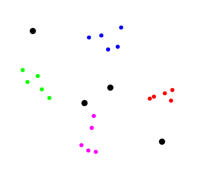
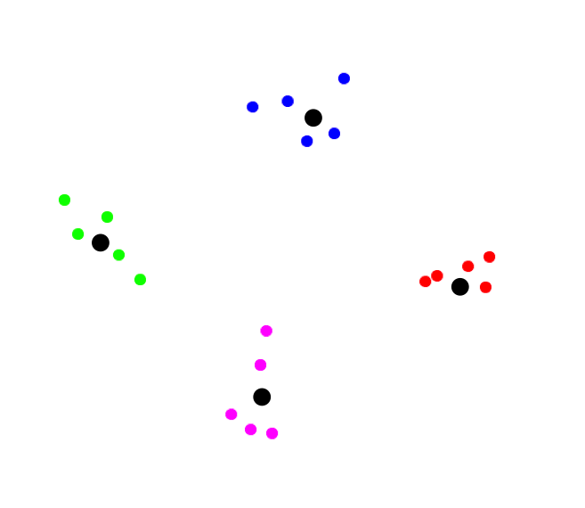
In-Class Exercise 24:
Execute DataExample3 to see an example of raw
data in four clusters. Then execute PCAExample3
to see that the clusters carry over to PCA coordinates.
Clustering algorithms:
- There are many popular clustering algorithms, a full
description of which would take us off topic.
- We'll instead present two high level ideas:
- Clustering using centers
- Clustering using hyperplanes
- Using centers:
- Start with some random "centers":
- Iterate, moving centers, until the centers stabilize:
The algorithm works like this:
     Algorithm: kMeans (X, K)
     Input: data points in columns of X, number of clusters K
     1.   find initial locations for K centroids
     2.   while centers not stabilized
              // Assignment to centroids
     3.       for each point xi
     4.           assign to cluster associated with closest centroid
     5.       endfor
              // Recompute centroid locations
     6.       for each cluster
     7.           cluster centroid = average of coordinates in cluster
     8.       endfor
     9.   endwhile
     10.  return clusters
- Hyperplane algorithms seek to find hyperplanes that
divide up the points so that each cluster can be separated:
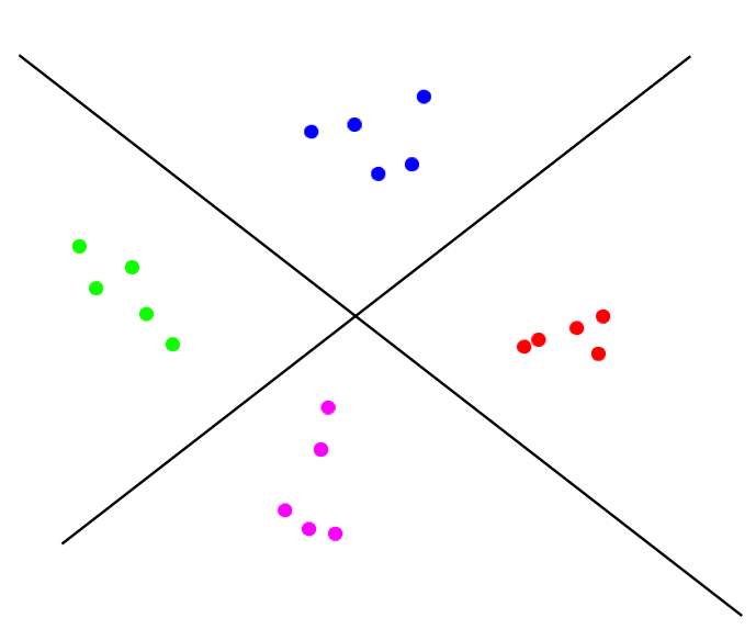
- Hyperplane separation is a staple of machine-learning:
- Neural networks
- Support vector machines
- Logistic regression
- We will be less concerned about how these algorithms work
than with pre-processing the data via PCA to make them
work well.
A difficult clustering problem:
- Sometimes the data can be inherently difficult to separate
via planes or centers, even if the clusters are obvious.
In-Class Exercise 25:
Execute DataExample4 to see an example of raw
data in two obvious clusters.
Explain why a couple of hyperplanes won't work to separate
the data. Also explain what could go wrong with the
K-means algorithm.
- In preprocessing the data, we could apply PCA
to get new coordinates and cluster based on those coordinates.
In-Class Exercise 26:
Execute PCAExample4 to see what PCA does
for clustering. Are the PCA-transformed points
easier to cluster?
- Unfortunately, direct PCA doesn't help either.
- The fundamental problem is that the two clusters are
inherently non-linear, while PCA is a linear transformation
that will preserve the non-linearity in the data.
- What we need: a nonlinear version of PCA.
In-Class Exercise 27:
Execute KernelPCAExample to see the transformation
achieved by Kernel-PCA.
Are these points easier to cluster?
Kernel-PCA:
A similarity kernel function:
Summary:
- With PCA and kernel-PCA, we have dipped our toes into the vast
field called machine learning.
- Linear algebra is a key building block of that field.
- Even though the ideas above are simple to apply, their
effectiveness on actual problems is varied.
- Often a combinations of tools is needed to really ferret out
the valuable patterns in data.
- Just as kernel-PCA is a non-linear version of the
linear PCA, there are other non-linear methods for dimension
reduction that are computationally intensive but have proven useful.
One such popular method is TSNE (you can read about it).
